GeistHaus
log in · sign up

Xander’s Scribblings

Part of xenendev.github.io

Essays, ideas, and explorations in technology, mathematics, and creative thinking

stories primary
ClassroomFeed Is Up: Time For a Breakdown!
aiedtechprojectproductivity
Announcing ClassroomFeed, a service that connects to Google Classroom and delivers weekly, AI-generated summaries for students and teachers. I also break down some key architectural design choices.
Show full content
ClassroomFeed Is Up!

So, I finally polished everything to a standard quite far above MVP. I’ll still be working on the reflection system and AI chat features. However, the core functionality is working.

Here’s the the producthunt page: https://www.producthunt.com/products/classroomfeed

And the website itself: https://classroomfeed.com

Here’s a little ad section for you

ClassroomFeed connects to your Google Classroom and sends you a weekly email with an AI-generated summary of:

  • Upcoming assignments
  • Completed work
  • Productivity patterns and streaks
  • Motivational prompts to reflect and plan ahead

It’s like a personalized weekly “check-in” powered by GPT, tailored to your school data.

Who is it for?
  • Students (especially high school, IB, or AP) who use Google Classroom and feel overwhelmed by scattered due dates
  • Parents, counselors, or teachers who want passive insight into student progress
Why I built it

As an IB student, I constantly missed due dates because Google Classroom has no unified weekly view. I built ClassroomFeed to make my academic life less chaotic—and realized it could help others too.

The Design Details

The SaaS was built using my bread and butter react, express but this time I had to split the backend between 2 systems: A Flask running python instance and the express backend.

Architecting this system came with quite a few fascinating design paradigms to consider. I’d say that’s the one of the biggest things I learnt from this.

Tech Stack To Recap
  • Frontend: React.js
  • Backend: Node.js, MySQL, GPT-5 API
  • Auth: Google OAuth (Classroom API) + JWT
  • Emails: Mailgun
  • Hosting: Vercel, Railway

The primary hurdle was figuring out what backend systems belonged on the Python server and which on the express.js one.

I first split them cleanly.

Express.js Server
  • All the backend routes accessable to the frontend
  • User authentication
  • User data storage (database access)
  • Cron job and event triggering
  • Account changes
  • Storing and creating the OAuth token for each user
Python Server (flask)
  • Handled AI (GPT-5) Integration
  • Google Classroom ‘scraping’
  • All Email Sending

So the lines were pretty clearly drawn. The MySQL database acted as a clear shared ground between the 2 systems.

But then I gave the user the option to trigger an email to be sent, and invite their parents to recieve copies.

Things got more sticky.

If the user requests sends an invitational email to their parents, the express server does the auth, handles rate limiting. But… at some point the express server must inform the python server to send an email.

I considered creating some sort of “send an invite email?” flag in the database that the python server would contiually check for:

[User] ---send invite email>>> [Express Server] -> [DB]
[Python Flask Server] -?> [DB] if so, send email

That could’ve worked but seemed a little too contrived.

Allowing the express server to just handle email sending could’ve worked too. But that was a pain.

So I settled on a little cross-server axios magic I managed to figure out. With the system now implemented, the request from the user gets passed down to the python server.

Note the separation of responsibility:

  • The express server validates, generates an invite link, and then forwards those things in a neat request to the python server.

This means the python server could just focus on email sending logic instead of cumbersome validation and database querying.

My Next Hurdles

I still tackled the reflection and email sending systems. Let me diagram how they work, and why I arrived on those designs.

From a higher level:

Node.js Scheduler/User Action
⬇︎
Node.js API
- DB lookup
- Prepare POST payload
⬇︎
Python Server (Flask)
- Validate input
- Queue background task
- Fetch/Analyze data
- Generate summary with OpenAI
- Send email
- POST/PATCH result to Node.js (update DB)
⬇︎
Node.js
Update status/record
Admin/email monitoring and error handling

The expressJs server does the queueing through a 15 minute cronJob. If it finds a scheduled email for a user in that 15 minute slot, it dispatches the axios request to the Python server:

cron.schedule('0 9 * * 1', async () => {
  // This function runs on schedule
  const [pendingEmails] = await pool.query(
  "SELECT * FROM users WHERE send_schedule = now ..."
  );

  for email in pendingEmails {
    await axios.post('http://python-server/api/deliver-email', {
        email: ...,
        first_name: ...,
        last_name: ...,
        google_refresh_token: ...,
        // other fields...
    }, {
        headers: { 'X-API-KEY': 'abcxyz' }
    });
  }
});

Then across the fibreglass wires, our Python server recieves:

@require_api_key
def deliver_email():
    # Receives POSTed JSON, validates, then queues background email generation. Perfect nugget of data!
    queue_email_generation(user_data)

where queue_email_generation() may look like:

def queue_email_generation(user_data):
    start_thread(send_weekly_digest(user_data))

async def send_weekly_digest(user_data):
    # 1. Extract fields from user_data
    get recipient email, name, google_refresh_token, preferences, etc.
    
    # 3. Gather and analyze classroom data
    classroom_report = classroom.scrape(token)
    
    # 4. Generate email content using AI
    email_body_html = writing_agent.write_email_body(
        # Classroom Data, user prefs, etc. data...
    )
    
    subject = "ClassroomFeed Weekly Report for {first_name}"
    
    # 5. Generate reflection questions
    reflection_questions = writing_agent.create_reflection(
        # top secret data
    )
    reflection_url = make_post_request_for_reflection(reflection_questions)
    
    # 6. Personalize and assemble email content
    # Replace unsubscribe link, reflection URLs, footer, etc. into email_body_html
    
    # 7. Send the email
    email_client.send_email(
        from, to, subject, email_body_html, cc_emails, etc.
    )
    
    # 8. Handle copied recipient emails
    
    # 9. Handle errors and log results

    # 10. Send email content and sending status back to expressJs server.

Note that because email generation takes a long time the express server doesn’t recieve a response to the python/api/deliver-email endpoint after the email is sent to the user.

Instead, the Python server ‘reports’ back after it’s done, and the express server stores the email sent, updates internal states, and marks the email as resolved.

request → acknowledge → async process → callback (once done)

I realized some of this back and forth information hot potato act going on was a little confusing and not the cleanest design pattern, simply because I wanted to stick to that orginal seperation of responsibility. Like I didn’t want the python server to read from database or perform state updates.

I could’ve also built the entire thing in python (or flask), but I was just going off what I was comfortable in coding with. Express.js was my backend go to, and Python was were the AI coding happened - and where I built the first functionality of ClassroomFeed’s AI system.

The Reflection System!

This was a nice little nugget of a system to craft on the side, because I most of the reflection sits nealty inside the email generation system. The halfway through preparing the weekly email, a ‘reflection’ is generated with the python server utils.

Then, as the email needs to contain a URL to access and respond to those reflection links, the python server posts this reflection to the express server. Basically making an instance of a reflection, containing the questions, comments, who its for, etc.

Express server then replies with a URL, which is a link that open to a form where a student can complete this reflection - the “reflection access link”.

Python server then slides that reflection access link into the user’s email before sending it off.

For a moment, can we just acknowledge how cool JWT’s are. I didn’t use them for identity or auth only. They served as links to the reflection lists. Invite links. The magic of cryptography means I don’t need to carry a bunch of extra internal states.

Essentially, I like to think of the reflection system as a little sub process that starts and ends within the wider email generation pipeline:

Spawned during generation
Stored by Express
Injected back into the email
Completed asynchronously by the user (independant)
A Wider View of The Reflection Pipeline

flow_diagram

Takeaways!?

So making ClassroomFeed made me really question whether clean separation of responsibility is more valuable than minimal component count, even when it introduces extra inter-service communication.

The answer: I still don’t know. But, databases are not certainly not message queues. I’m glad I didn’t use my database as a messanger or shared state container. In the actual production system, the python server doesn’t even touch the database.

This clear separation of responsibility, may have impacted technical complexity, with the cross-service requests and extra validation checks. Regardless, having the clear responsibility seperation between these services was a more important. And I saved the need to write a lot of boiler plate that would be shared between the python and express servers.

The one thing that wasn’t an issue but could be, and was on my mind, was that if a packet failed or dropped in the cross-service talk, it could lead to a hard failure. I did implement retry logic, but frankly any networking code, with all its retry, and validation checks becomes a little bulky.

In short I’d say:

For:
  • Python never needs DB reads
  • Python never needs permission logic
  • Python becomes a deterministic execution engine

This made it simple.

Strict separation of concerns: Express owns state, identity, and orchestration; Python owns computation and side-effects. No conceptual leakage.

Python becomes a pure execution service: given an input payload, it deterministically produces output and reports results. That is an ideal AI worker model.

Zero persistence coupling in Python: no schemas, migrations, or transactional logic contaminating the AI layer.

Zero security surface area in Python: no authentication, permission hierarchies, or rate limiting logic to maintain.

Express becomes the single source of truth for system state, which prevents split-brain data ownership.

The Python service is stateless and horizontally scalable by default.

Failures become isolatable: AI bugs do not corrupt user state, and DB bugs do not poison AI execution.

The API boundary becomes an explicit contract, which enforces architectural discipline.

AI is treated as a computational primitive, not as an application core.

The system naturally evolves toward event-driven design, even without formal message brokers.

You gain technology freedom: either side can be rewritten, scaled, or replaced independently.

Testing becomes cleaner:

Express tests validate business logic and persistence.

Python tests validate transformation correctness.

Against:

Increased orchestration overhead: every meaningful action now requires cross-service coordination, which multiplies failure modes and debugging complexity.

Higher latency surfaces: even trivial operations become multi-hop HTTP transactions instead of in-process calls.

Harder observability: tracing causality across Express → Python → Express requires structured logging, correlation IDs, and disciplined telemetry.

More infrastructure fragility: two servers means duplicated deployment pipelines, health checks, and version compatibility risks.

Tighter contract coupling: any schema change in request or response payloads must be synchronized between services.

Non-trivial error choreography: partial failures demand compensating actions instead of simple exception handling.

Higher mental load: the system becomes conceptually distributed, even if deployed on a single machine.

Overhead in local development: you now need multiple processes, environment variables, and mocks just to test a single feature.

Closing

Thanks for reading all this way. Seriously. If anything made sense, I’m glad. So here’s this majestic near complete flow chart of the entire core system of ClassroomFeed (It’s still missing a bunch of small features and intracicies).

flow_diagram

https://xenendev.github.io/posts/classroomfeed-ai-summaries
Why Logic Belongs in Prompts, Not Code: What I Learned Creating A Broken Agentic System
agentic-aillm-systemsai-engineeringsystem-designprogramming-philosophy
A hands-on case study of redesigning an LLM-driven school announcement system, contrasting brittle procedural pipelines with agentic architectures. I detail the failure modes, prompt engineering, tool loops, stress tests, and a reproducible agentic blueprint—explaining tradeoffs, debugging patterns, and advice for building robust, maintainable LLM-powered systems that can reason and take actions safely.
Show full content

After shipping my AI-powered automated school announcement board, I had a problem: it was unmaintainable, undebuggable, and rather stupid. I re-architected the whole thing into an agentic system. The system exhibited far superior functionality while going from ~1,750 words to ~550 words of core system prompting. It was 10x more flexible at handling edge cases. I no longer got questionable results from a Tuesday scheduled cron job.

This is a breakdown of a real LLM-powered system I built, broke, and rebuilt. The differences in my first and second iteration changed how I approach programming AI systems today.

I’ll walk you through the process that led to my redesign, demonstrating its advantages and comparing it to the original procedural approach. We’ll then generalize these insights and provide a beginner’s guide to the approach I use when designing automated AI systems.

If you’re building LLM-based tools and running into edge cases or poor AI decision making, this post could be the key to addressing that. If you’re already building agentic AI systems, some of this might feel obvious. But I think going back to why we do something in the first place can be useful. We’ll also try to understand where and why my initial design excels.

Table of Contents Setting The Scene

I had developed a centralized digital school notices and upcoming events board (visible through a website) for my school. My next piece in this system was automated processing: take school announcements from Google Classroom (my school’s native platform where teachers post announcements and assignments) and post them to our digital notice board.

At first, I sketched out what seemed like a sensible high-level plan with basic procedural steps:

  1. Poll Google Classroom for new announcements every 15 minutes (cron job)
  2. Decide whether each new announcement should be an event or notice on the board (LLM prompt)
  3. Summarize, shorten and formalize the announcements (another LLM task)
  4. Pick appropriate dates for showing/removing the announcement (with an LLM)
  5. Post to my announcement board

I thought: “Perfect! I’ll use an LLM for all these semantic, iffy evaluation tasks. I’ll just need some prompts and output validation.” Straightforward enough.

Here’s essentially what that initial process looked like in code:

function process_announcements():  
    new_announcements = check_for_new_announcements()

    for each announcement in new_announcements:

        # Step 1: Classify announcement  
        post_type = LLM("Is this an event or a notice?", announcement.text)

        # Step 2: Check for duplicates  
        existing_items = get_existing_posts(post_type)  
        is_duplicate = LLM("Is this announcement a duplicate?",   
                           new=announcement.text, existing=existing_items)

        if is_duplicate:  
            mark_as_processed(announcement.id)  
            continue

        # Step 3: Extract and format data  
        post_data = LLM("Extract title, description, dates, target years",   
                        announcement.text)

        if missing_required_fields(post_data):  
            log_error("Missing fields in announcement", announcement.id)  
            continue

        # Step 4: Post to backend  
        if post_type == "notice":  
            post_to_api("/api/notices", post_data)  
        else:  
            post_to_api("/api/events", post_data)

        mark_as_processed(announcement.id)

Notice the structure: how each step is isolated, makes an LLM call, validates the output, and passes data to the next step. It seemed logical, I cleanly separated concerns and tasks, making it easy to debug each step. Classic software engineering principles.

The Breaking Point

The initial approach worked, until it didn’t. I learned that Google Classroom announcements are a mess of edge cases waiting to break everything. Soon my 5-step pipeline had to handle announcements that:

  • Were corrections to previous posts: “The assembly is at 2pm, not 1:30!”
  • Weren’t relevant: “John and Sarah, please come collect your textbooks”
  • Contained multiple individual notices: “Here’s some notices for the week: …”
  • Had vital context in attached images: “Check the attached image for this week’s schedule”
  • Were both an event AND a notice
  • Were duplicates posted across classes at once
  • Should be merged with existing board items, not posted separately
  • And more!

My instinct as a systems-oriented programmer was to treat each exception as a branch in the logic. So I started creating more functions to address each edge case:

def check_if_merging_announcements_are_suitable(announcement, existing_notices):

    """Prompt the LLM, asking it to assess if this notice should be merged  
    with an existing one based on the current notice board"""

    prompt = f"""..."""  # Another verbose, context-stuffing prompt

    response = call_llm(prompt)

    # Sanitize and extract the final judgement  
    # Convert from string to data type  
    # Error handling  
    # ...

Very quickly, the once-straightforward looked like:

└── For each recent announcement:  
    ├── Check if already processed  
    ├── If new/updated → Process announcement:  
    │   ├── Extract text and materials (files, links, videos)  
    │   ├── AI Relevance Check: Is this suitable for notice board?  
    │   │   └── If not suitable → Skip and mark as processed  
    │   ├── AI Classification: Is this an "event" or "notice"?  
    │   ├── Duplicate Detection:  
    │   │   ├── Query existing notices/events from backend  
    │   │   ├── AI comparison to find duplicates  
    │   │   └── If duplicate → Update targets or skip  
    │   ├── Content Processing:  
    │   │   ├── Determine dates to show notice / event  
    │   │   ├── AI content condensation, formatting and formalizing  
    │   │   └── Create structured JSON (title, description, dates)  
    │   └── Post to backend  
    └── Continue to next announcement

Though tedious, I tried to create a branch of logic for every random post, silly announcement, and mistake that could occur. By the end, my code became a mountainous heap of if statements and LLM task evaluation functions, bound by the rigid, stepwise process I outlined to solve the once-seemingly straightforward problem.

Yet even still, I’d get the occasional 2 p.m. email from Render.com saying my service failed, and mornings where duplicate announcements had snuck through.

If I wanted something flexible, dependable and airtight, this wasn’t it.

The Realization

The solution slowly became clear when I began distancing myself from the problem: I was treating this like a programmer would, so I stepped back and thought about how a human would solve it. It made me realize I was writing logic in the wrong language.

I was still programming like the machine needed rigid instructions. Like I was writing code, not using reasoning. But LLMs don’t operate like CPUs. They don’t follow deterministic execution; their superpower is holistic reasoning, contextualization, and inference.

When I placed an LLM in the role of evaluating a single statement (e.g. ‘determine if this post is suitable for the board, yes or no?’), I was feeding it tunnel-visioned tasks as part of some bigger pipeline, while attempting to stuff enough context through verbose prompting so it could do a half-decent job.

This approach brought a plethora of issues:

Fixing behavior was hell: You didn’t know what the AI was thinking to arrive at a decision (because really, it wasn’t thinking much). When a final action was unexpected, it was rarely clear which step was the culprit. That’s a problem with long dependency chains in general: every link must work perfectly; if one breaks or misbehaves, the whole system fails.

Each step lacked context: Only from a distance could we see why one choice didn’t make sense in the wider context. These AI tasks were tunnel-visioned badly. Thus, blind to the full task, they were unable to make reasonable choices.

Prompts became verbose and inefficient: Writing and tweaking prompts became a chore. Having higher OpenAI API bills each month wasn’t nice either.

Edge cases were inevitable: It would eventually encounter something the system wasn’t designed for, a branch in the code that didn’t exist.

Like an inefficient corporate middle-management system, we needed a to de-stratify the thing. I had to treat the LLMs like I was handing a tasks to a humans. I think I didn’t see this because I was too used to thinking like a ‘classical’ programmer.

The Agentic Redesign

After going back to the drawing board, I understood that breaking down the problem into 25 pieces wasn’t the method. The solution was blatantly simple (and scarily easy): describe the entire problem in a single LLM prompt and provide it with the tools that any human doing the same task would need (e.g. post to backend, check existing board, query classroom data). This is essentially the nucleus of agentic design: providing agency.

This architecture reframes the LLM at the center of the task, not the code. In this architecture, the LLM runs creates the logic, and it isn’t hard-coded into the program.

Here’s the agentic AI system that came out of that:

├── Fetch Data  
│   ├── Announcements + assignments from Classroom  
│   └── Current state of board (notices + events)  
│  
├── Construct Agent Context  
│   └── Compile prompt with environment, data, and operational rules  
│  
├── Agent Loop (≤ 8 iterations)  
│   ├── Sonnet-4 receives full context and available tools  
│   ├── Chooses tools, executes functions, reasoning is logged  
│   ├── Receives updated state + conversation history  
│   └── Re-evaluates until calling `finish_processing()` or max steps  
│  
├── Available Agent Tools:  
│   ├── Information Gathering:  
│   │   ├── get_announcements() → Latest classroom announcements  
│   │   ├── get_assignments() → Upcoming assignments  
│   │   ├── get_existing_notices() → Current notice board  
│   │   └── get_existing_events() → Current events board  
│   ├── Content Management:  
│   │   ├── create_notice(title, desc, dates, targets)  
│   │   ├── update_notice(id, title, desc, dates, targets)  
│   │   ├── delete_notice(id)  
│   │   ├── create_event(name, desc, date)  
│   │   ├── update_event(id, name, desc, date)  
│   │   └── delete_event(id)  
│   └── Session Control:  
│       └── finish_processing(message) → End with summary  
│  
└── Terminate  
    ├── Agent ends session or times out  
    └── Return summary of actions taken

I learnt these things while redesigning:

  • The code itself became far simpler because I could neatly separate API and tool functionality with the AI prompting, as opposed to having them mix throughout the code, like with the procedural design.

  • Leveraging tool calling and large context windows was key. High-agency models trained for tool use, like Anthropic’s Sonnet 4 (and now 4.5), were particularly impressive with this task.

  • I found it interesting how the second iteration wasn’t too dissimilar from the original draft solution. I still kept that branch-like conditional structure, although expressed in prompt, not code, by describing the decision-making procedure to the agent.

The paradigm shift is was sneaky: put the logic and decision-making into the LLM, not the code.

I like to think of it as treating the system like a human employee (but with steering and guardrails).

Comparison I made this illustration to show the general architecture of both types of systems, agentic and procedural.

What I Learnt From Prompting

Good prompting was core to the success of this agent (and any other agent). Here’s the core system prompt I refined through lots of testing:

You are a digital school board assistant for XXX School's 'Tutor Board' app. Your primary responsibility is to create, update, and manage notices and events based on data from the school's Google Classroom system.  
You have access to the following information:  
1. Current date and time:  
<current_date_time>{strftime('%Y-%m-%d %H:%M:%S')}</current_date_time>

2. Google Classroom data to process for today (announcements and assignments):  
{classroom_data}

3. Current state of the Tutor Board for reference and context:  
<current_board_state>{board_data}</current_board_state>  
Your task is to process this information and make appropriate updates to the   
Tutor Board. Follow these guidelines:

1. Analyze each item from the Google Classroom data:
   a. Determine if it's relevant for the Tutor Board
   b. Decide whether it should be a notice or an event
   c. Create or update the notice/event accordingly

2. Notice vs Event:
   - Notice: An announcement or information (e.g., new canteen rules)
   - Event: A specific date and time activity (e.g., bake sale, assembly)
   - Refer to the current board for good examples of how these are categorized

3. Clean up work:
   - Consider if new information can be merged with existing events/notices
   - If a notice is outdated or irrelevant, remove it from the board
   - Delete notices/events that are no longer relevant or have expired

4. Manage duplicates:
   - Remove or merge duplicate notices/events as needed
   - Avoid unnecessary modifications to existing entries

5. Formatting requirements:
   - Links: Use [URL title](URL) format
   - Description: Keep under 1024 characters
   - Title: Keep under 80 characters
   - Remove sensitive information (full names, passwords, private details)

6. Dates:
   - Infer start and end dates from context
   - For notices, aim for shorter timeframes (rarely longer than 1 week)

7. Target year groups:
   - Assign appropriate year groups based on context
   - IB Notices: Years 12 and 13
   - Key Stage 3: Years 7, 8, and 9
   - Key Stage 4: Years 10 and 11
   - Default: All year groups (7-13) if unclear

8. Tool usage:
   - You have 8 'rounds' of tool calling. You must plan and finish within that budget
   - Run tool calls concurrently when possible
   - If a tool call fails, try once more before moving on
   - Use finish_processing when all suitable changes are made

After processing, use finish_processing and provide a recap of actions taken.
Remember: you have autonomy to organize the Tutor Board. This includes merging 
information, removing outdated content, or updating existing items based on new 
information from Google classroom. Notice how events and notices are currently categorized and written on the board and maintain that consistency.

A pattern in prompt design I discovered from this is to tell the model to self reference its own previous outputs to understand conventions and expectations of the task. The agent then feeds into these existing implicit patterns on the board, which makes outputs less random and more consistent across different scenarios.

This leads to less unpredictable and incongruent behavior of the agent. A simple “refer to the current board for good examples” or “notice how events and notices are currently categorized” works to keep behavior stable. This is a useful prompting pattern I haven’t seen talked about.

Another important thing: guiding the reasoning with a procedure was detrimental to the quality of the output. Forcing the model to reason through each consideration one by one made it not glaze over anything. Guidelines also reduce the agent going haywire with tool calls, thinking it needs to do more than it should. I’ve noticed models can act too high-agency sometimes and cause issues.

In short:

  • Try to fit in a self-referential pattern; this is where the model gets fed examples of its own past actions
  • Give as much context up front, and importantly, how to that content. I gave it the date and when to use it: “Infer start and end dates from context”, I find sometimes the models ‘disregard’ crucial context you’ve provided without this.
  • Guide it through the logical steps. A logical and procedural outline is still detrimental, write out the thought-process in the prompt.
  • Control agency (or the model’s reflex to want to do things) with guidelines. Otherwise, it doesn’t know what to do and starts calling all sorts of tools. I’ve seen things get out of control this way. “
A Comparison With a Real Scenario

Let’s test both systems with a real announcement that would’ve broke my procedural system. Our tricky announcement:

  • contains multiple items
  • a password that needs removal
  • a duplicate topic
  • and a scheduling conflict.

Real nasty.

Test announcement:

Hey all, 3 announcements for today:

MATH COMPETITION: Saturday, Feb 5th. Sign up by Jan 28th.

REMINDER: All students must complete math revision online. Login with password “school5”.

CLUB MEETING: Environmental Club meeting next week on Tuesday Jan 18th, 3:30 PM. The Student Council meeting will be moved to after the meeting.

Existing board state:

  • Notice: Year 10 Community Service Hours Reminder
  • Event: Student Council Meeting (Tuesday, Jan 18th, 3:30 PM)
Procedural System: Catastrophic Failure

When following the rigid pipeline, the system couldn’t separate the three announcements. Instead, it classified everything as a single “event” and then got confused by the Student Council mention and flagged it as a duplicate.

Result: 2 out of 3 announcements lost entirely.

Agentic System: Handled Everything

In just two iterations, the agent:

  • Created Math Competition event with correct details
  • Recognized the community service reminder was already posted (no duplicate!)
  • Removed the password when updating the existing notice
  • Created the Environmental Action Group event
  • Updated Student Council meeting time to resolve the conflict

The difference? The agentic system could understand the relationship between information. It saw the scheduling conflict, caught the security issue, and knew when to merge instead of create. Meanwhile, the procedural system followed its tunnel-visioned steps and failed.

This is the kind of nuanced, context-aware decision-making that requires reasoning across the full problem space. Something procedural pipelines fundamentally can’t do.

Tradeoffs and When to Use Each Approach

Spectrum

TL;DR

The rule of thumb I’ve come to use is simple: if you can describe the logic clearly, go procedural; if you can’t describe the logic but can describe the goal, go agentic.

In short:

  • When latency matters: User-facing applications where response times are critical can favor procedural approaches.
  • When cost matters: Simple, repetitive tasks where the procedural approach works well might not justify the expanded cost of agentic thinking and reasoning turns.
  • When you need determinism: Like in financial systems, medical decisions, compliance-heavy domains. Essentially, anywhere you need to prove exactly why a decision was made (procedural decision trees are easy to log) or require the same input to be consistently handed the same.
  • When you need flexibility: Content moderation, creative tasks, fuzzy classification problems, anything with changing requirements as agentic approaches can adapt without code changes.

Use procedural LLM pipelines when you:

  • Have a well-defined problem with known edge cases
  • Need deterministic, auditable decisions
  • Require fast response times and minimal cost
  • Can achieve high accuracy with simple prompts
  • Need to satisfy compliance requirements

Examples: data extraction from invoices, sentiment analysis, simple classification tasks, batch processing with known input formats.

Use agentic approaches when you:

  • Face many edge cases and evolving requirements
  • Need contextual reasoning across multiple pieces of information
  • Can tolerate slightly higher latency and cost
  • Want the system to adapt without constant code updates
  • Have tasks that humans do by “using good judgment”
When Procedural Still Wins

I think procedural designs address a narrow type of problem; between ones straightforward enough that LLMs aren’t required, and problems too dynamic and semantic (like my notice board). Though somewhat outside the context of automation, NLP tasks are a good example of problems that procedural systems work well, as LLMs are just leveraged for their ability to understand language and meaning, but not their planning and decision making capabilities.

Because procedural is cheaper, faster and deterministic, systems needing low latency or high processing capacity could advantage from procedural.

I think the choice between architectures ultimately comes down to the nature of the task itself: If the task is deterministic, simple, and well-bounded (where the logic can be described step by step and the outcome is always predictable) a procedural system is the clear choice. These are situations where speed, cost, and reliability matter most, and where ambiguity or open-ended reasoning would only introduce unnecessary noise. Think data formatting, validation, fixed-scope NLP tasks like summarization or sentiment classification, or any workflow that repeats identically at scale. The strength of a procedural pipeline is its stability: it’s faster, cheaper, and straightforward to debug, with no risk of runaway reasoning or unexpected autonomy.

On Agentic

One issue with agentic design: putting too much agency and trust in a single system may raise concerns about reliability, security and safety. My school notice board was innocent enough that I had little concerns with this. However in cases where airtight reliability is needed, the system I implemented would not be ideal. Interesting hybrid systems exist that can still combine agentic’s strengths. For example, a system consisting of a moderator and agent running in tandem where the agent carries out its task, and the moderator independently approves the final proposed course of action from the agent.

However, when a task begins to involve interpretation, contextual awareness, or the need to make nuanced decisions that can’t be captured by rigid conditionals, an agentic system starts to make more sense. These are problems where the “right” answer depends on judgment and the relationships between pieces of information rather than just the information itself. Agentic systems excel at this kind of reasoning because they adapt, merge, reorganize, and infer. They’re ideal for messy, dynamic tasks like content curation, information synthesis, contextual automation, or systems that must act based on partial or evolving data. Instead of being told exactly what to do, the AI is told what goal to achieve and given the tools to get there, just like a capable human employee operating under broad but clear guidelines.

In practice, though finding where the procedural pipeline went wrong was easy, I found fixing behavior in the agentic system to be easier for my system because I could understand and address the agent’s reasoning after seeing it: “I’m merging these two notices because they cover the same topic.” The procedural system just failed silently or produced wrong results with no explanation.

Exploring Hybrid and Designs

When I worked on a newsletter synthesis pipeline, the context usually was too large and would overload the agentic pipeline. It forgot to do things, took shortcuts in reasoning and lost its decision making fidelity in general. I’m not sure exactly at what point this occurs, but my rule of thumb is, if it’s a complex task that can be neatly broken down into stages, consider using a hybrid procedural-agentic pipeline, where the task is split into a pipeline of agents or simple tasks. Each agentic agent in the pipeline has a manageable task where outside context is irrelevant in the execution of said task. For example, the part of my newsletter pipeline that scored each article across several metrics (relevance, trustworthiness, interest factor, etc.) was a single agent; the other steps in the pipeline to craft a newsletter benefitted from not having to think through the rating process and could focus more on the writing.

A practical application of a hybrid system is for security. For my notice board agent, I simply asked it to omit any PII or confidential information in its posts. However, in hindsight, trusting an agent, burdened with many other responsibilities, with such an important requirement, was not a great idea. Here’s where a pre-processing screening agent, which has the sole and only purpose of censoring any sensitive information before passing it on to the agent, would have been the most secure. This step could also screen prompts for potential prompt injection attempts, especially when a prompt injection for an autonomous agent could literally be catastrophic. Generalizing this, a lot of ‘specialist’ tasks that are important or require specific and careful instructions may benefit from being separated from the main task in a pipeline.

For security, a useful heuristic is that the more agency a single agent possesses, the more catastrophic its failures can become. A high-agency system with wide tool access is powerful but also harder to constrain or audit. When safety is critical, consider decomposing a high-agency task into smaller agents with limited tool permissions. You lose some of the holistic reasoning and adaptability of a fully agentic design, but you gain determinism and containment. It functions like an airlock: isolating potential failure before it spreads through the system. A human in the loop system can also be emulated: using another antagonistic agent, have it audit the process and be an overseer of the first agent. Be cautious though, prompting requires fine tuning the attitude of both agents. You don’t want the overseer being too relaxed or strict and cynical.

Consider also for some systems: having a router (could be a cheap model or rule engine) that decides whether the task should go down the procedural pipeline or the agentic one if a higher caliber of fidelity is demanded and otherwise cost or latency is important.

Spectrum 
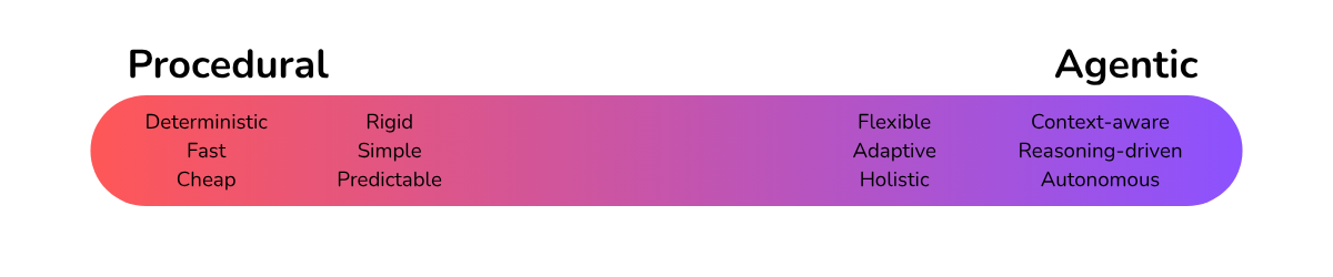
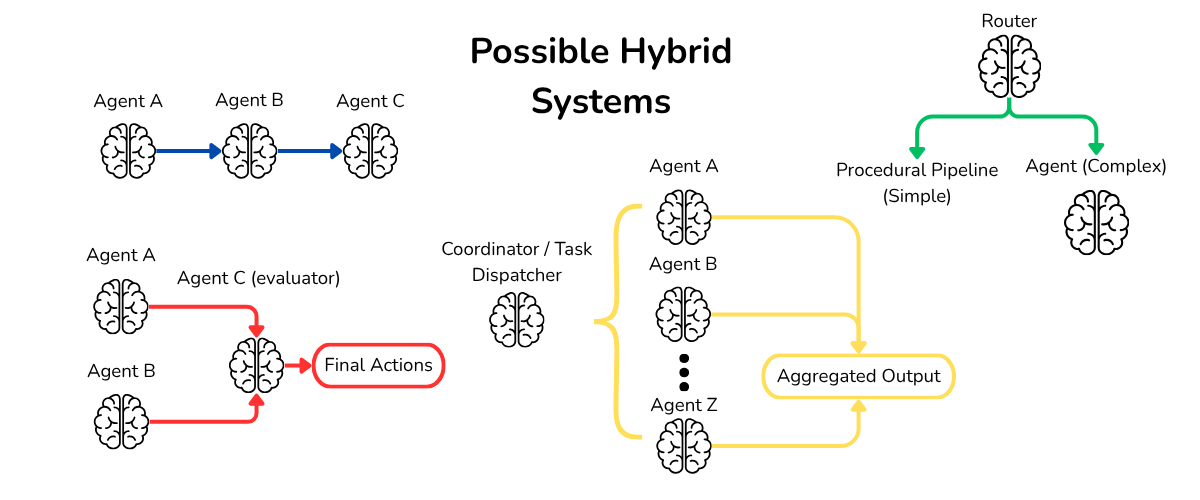
There’s really a bunch of interesting structures you can make, many mirroring real world organizational structures. I’ve illustrated just a few, ones which I’ve implemented in some form.

When designing the architecture to solve the issue, I’d recommend looking from the top. Assume the entire goal is described in one prompt, then subdivide it from there, seeing which parts of the task may benefit from being a dedicated task.

Candidates for separation may include:

  • Tasks requiring strict determinism or measurable criteria (e.g., data validation, format checking, PII redaction)
  • Components that operate on distinct or isolated context (e.g., scoring, filtering, summarizing independent chunks)
  • High-risk or security-critical processes that benefit from isolation and independent verification
  • Stages where tool usage or API interactions are consistent and well-defined
  • Subtasks that can be easily unit-tested or benchmarked independently
  • Steps where human oversight or explainability is particularly valuable

And against:

  • Tasks that rely on shared, interwoven context or long-range dependencies across inputs
  • Processes requiring creative synthesis or global reasoning (e.g., holistic writing, cross-referencing insights)
  • Workflows where tight latency and cost budgets make extra routing or agent overhead prohibitive
  • Systems where decision coherence across subtasks is crucial (e.g., maintaining consistent tone or persona)
  • Scenarios with fluid or ambiguous task boundaries where subdivision creates confusion rather than clarity

I found myself asking these questions when considering whether some hybrid approach is best: Break down the problem: “Can I break down my goal into smaller, still semantic and difficult tasks that will result in the goal being complete?” Consider and define task boundaries “Should I merge some of these tasks? Would a human excel if some tasks were considered one? Would 2 adjacent tasks overload or confuse a human if combined into one?” Consider context, tools, guidelines, processing procedure, considerations, prompting, etc. “For each task: How much does my agent need to know to deftly handle it?” Then separate context, define strictly the tools needed, prompt with guidelines and put restrictions on the number of tool calls. (and all the other prompting expectations)

So next time you’re building something, ask yourself: “agent or procedural or some combination of both?”

Consider using some combination of both if:

  • The goal is made up of smaller tasks that aren’t very context dependant
  • You want more control over each step of the process, without losing fidelity
  • Tasks would be separate if given to a human
  • You want certain specialists that excel at a specific task that can feed into the larger goal
  • You want to compare different views and results across agents
  • The task can vary between being very simple or complex and latency and token efficiency are high priority. (consider routing)
For Those Who Want Specific Implementation Advice, This Section is For You

Here, I’ll walk you through a best practices implementation of an agentic system. The key decisions, factors and tips to create an effective system, agentic or procedural.

Higher Level Overview

Plan a higher level model of your agent or system. Label your inputs, and your output or things you need the system to do. The juicy part is finding what goes in the middle; they are the gears that make the system function. I would begin with one agent. One large task, as described to a human. Outline tools, context, safety, prompt, guidelines and general steps or considerations for the agent to think through. Then see what parts can become their own dedicated sub tasks (remember: security, specialization, determinism, without comprising reasoning etc.) Consider a safety later too for censoring or otherwise pre-processing information.

Now, speaking from personal experience, I encourage you to find the extremes, the most complex, unlikely, beleaguered inputs or conditions, and run it in your head. Picture you were given the instructions and steps outlined, would you accomplish the goal? If not, fix the procedure or be more specific in the prompt.

Prompting

Moving on, the prompt. There’s plenty of good prompting guides out there. But the here’s something basic to go off of (you can see my example too):

  1. Role and persona
  2. Detailed goal outline
  3. Consideration steps and things to work through (procedural instructions)
  4. Examples (can be self-referential)
  5. Tool usage guidelines
  6. Information and input information (wrap in <tags> like <this> for prompt injection mitigation)
  7. Any reminders and emphasis

Specificity and context is key. Ensure the model understands any lingo or specific meanings of the input. Ensure it knows what to expect, the beats it should go through when reasoning, the constraints it has, how it should call its tool. Like writing to an English speaking alien.

LLM Models

High agency models, trained on tool calls, like grok-4, claude sonnet 4.5 are especially good at tasks involving them. If you find a model getting reluctant to call tools, or to make many things move to reach its goal, you can switch models, or fine tune behavior through prompting. In a lot of cases just saying “act high agency” or “don’t be afraid to use many tool calls” does it.

Tools and Agent Loop

The tools are what the model has available to it, ensuring they are type safe for the data types that the LLM will provide. Ensure they aren’t super powerful (e.g. instead of a tool for enabling command shell access, give tools that run predefined, safe shell commands)

The agent loop is a loop of planning actions and then running tools to execute them. Usually the number of maximum tool calls or loop iterations is limited to prevent larger than necessary changes. Ensure that the agent is informed of any limits beforehand.

The agent loop looks a little like this:

messages.append({role: "system", content: prompt + context_and_data})

repeat:
    response ← LLM.generate(input = messages, tools = TOOLS)

    for each tool_call in response.tool_calls:
        result ← execute(tool_call)
        messages.append({ role: "tool", content: result })

        if tool_call.name == "finish":
            stop loop

Logging and refinement

Logging and reasoning out-loud is also vital to the refinement process. Ensure that the agent is instructed to think and plan out-loud (or is using reasoning tokens) before using any tools. By seeing its thought process, you can find places to intervene or suggest behaviors in the prompt. You should also keep the out-loud thinking in the prompt, because it gives the model tokens to ‘think’ and plan. You’ll get better, more thought out action plans that way. I find it extremely useful to tell the model to run some form of report_actions tool, where it gives a summary of actions done; this allows for easy reviewing.

Then program it. then test it. Use normal inputs and scenarios, alongside the extreme cases you made. Does it function? Does it produce slightly cautious or low agency behavior? Does it take shortcuts in reasoning? Does it overlook things? The answer will be yes. And the solution is more prompting. Refinement is key.

Then test safety. Try to prompt inject it, given that you know the internal system prompt. Can you still do it? If so, you should tighten it. Can you sneak a password past it? Or a sneaky private sales figure?

By this point, you should be in a good place to start using the agent.

Overtime you may want to monitor for:

  • Actions-per-run, rejected-item rates, tool-failure counts
  • Cases where it fails or behaves unexpectedly
  • Drift in behavior
To Wrap It Up

TL;DR: Consider if you should write your logic in your prompt, not your code. The bread and butter of agentic systems is agency, the ability to decide and reason freely. You should provide the AI complete context, how to interpret the context in its role, tools, and autonomy within guidelines are tool limits to solve your problem. Stop thinking about AI as a programmer would, and start thinking about it as a boss giving instructions to a capable employee.

Also keep these principles in mind:

Context over fragmentation: Give the full picture, not tunnel-visioned tasks
Flexible tools over rigid steps: Let the AI choose its path
Guide the decision-making process: Describe considerations, not commands
Implicit examples over explicit rules: Show current board state for style/pattern learning
Trust but verify: Set boundaries (tool budgets, safety checks) but allow autonomy within them

The shift from procedural to agentic changed my approach to designing AI systems: I stopped asking “what steps does the computer need to follow?” and started asking “what would I tell a capable intern to do?”

Instead of writing increasingly complex validation logic, nested conditionals, and verbose context-stuffing prompts for each step. You might be better off making AI with code. Remember, they’re not CPUs executing instructions, but reasoning engines making inferences.

Give them the full picture. Give them tools. Let them figure it out. That’s the paradigm shift. And once you see it, you can’t unsee it.


If Your Interested In More

Recently, Anthropic released their investigation report into ‘the first reported AI-orchestrated cyber espionage campaign’. The attackers cleverly used an agentic-procedural hybrid system, where each agent was obfuscated from the full task, circumventing safety problems by breaking down the task. This ‘scoping’ of AI agent tasks to orchestrate a larger, malicious task is an exploit and reason one might choose the more procedural architecture. They demonstrate how the attackers executed their operation. Read their report.

Also very recently, Vercel published this blog post showing how cutting 80% of their agent’s tools actually improved performance dramatically. Instead of dozens of specific functions, they gave it one tool: the ability to run bash commands. This points to a broader pattern emerging in AI development, that as models grow more capable, the carefully designed tool ecosystems meant to support them are becoming constraints rather than enablers. We’re watching a developmental inflection point: what was once necessary scaffolding for limited reasoning is now friction for increasingly autonomous systems. The structured, tool-heavy architectures we built weren’t wrong but they were training wheels. I think the models are starting to ride without them.

https://xenendev.github.io/2025/12/18/tds-agentic-vs-procedural
Extensions
Jansen’s Linkage Optimization
mechanismsoptimizationengineeringjansen linkage
A rigorous comparative study of Gradient Descent, Genetic Algorithms and Simulated Annealing applied to Jansen’s 13-link mechanism. Describes experimental setup, RMSE objective, grid-search hyperparameter tuning, statistical analysis and convergence behavior—showing SA’s robustness on this multimodal inverse-kinematics problem and providing concrete guidance for mechanism optimization.
Show full content

If you want to read this paper, I highly suggest viewing the nicely formatted PDF version available here: Zenodo Publication

Image 1

A comparison of Genetic Algorithms (GA), Gradient Descent (GD) and Simulated Annealing (SA) and how they differ in effectiveness when optimizing linkage lengths of Jansen’s Linkage to achieve a desired foot trajectory

Authored by: Xander van Pelt
Table of Contents

Abstract 3

1.Introduction 3

2. Background Knowledge 6

2.1 Jansen’s Linkage 6

2.2 Gradient Descent 6

2.3 Genetic Algorithms 7

2.4 Simulated Annealing 8

2.5 Previous Comparative Studies 8

3. Methodology 9

3.1 Simulation Methodology 9

3.1.1 Linkage Representation and Foot Trajectory Computation 9

3.1.2 Target Foot Trajectory 11

3.1.3 Error measurement 12

3.1.4 Experimental Setup 14

3.2 Optimization Methods 14

3.2.1 Gradient Descent 15

3.2.2 Genetic Algorithm 16

3.2.3 Simulated Annealing 17

3.3 Hyperparameter Testing 18

3.3.1 Gradient Descent 18

3.3.2 Genetic Algorithm 21

3.3.3 Simulated Annealing 25

4. Results 28

4.1 Convergence Behavior 28

4.2 Final Performance Comparison 29

4.3 Computational Efficiency 29

4.5 Qualitative Trajectory Analysis 30

5. Discussion 31

5.1 Main Findings 31

5.2 Implications for Linkage Optimization 32

5.3 Comparison with Literature 33

5.4 Limitations 33

Works Cited 34

Abstract

Jansen’s linkage, a planar thirteen-bar mechanism designed by Theo Jansen in the 1990s, converts rotary motion into efficient walking gaits for legged robotics. This study compares three canonical optimization algorithms, Gradient Descent (GD), Genetic Algorithm (GA), and Simulated Annealing (SA), at their effectiveness for minimizing trajectory deviation from a target effector trajectory (gait).

Each algorithm optimized thirteen linkage bar lengths to minimize root mean square error (RMSE) between simulated and target foot trajectories, sampled at 180 points per crank rotation, under identical evaluation budgets of 100,000 objective function calls. Each method executed 200 independent trials with randomly initialized semi-feasible configurations.

Hyperparameter selection employed systematic grid search with statistical validation confirming robustness. ANOVA analysis revealed that run-to-run initialization variability exceeded hyperparameter-induced variance by 5-7× across all algorithms (η² < 0.03, p > 0.05), establishing that observed performance differences reflect fundamental algorithmic characteristics rather than tuning choices.

SA achieved median RMSE of 1.08 units, significantly outperforming GD (3.68 units) and GA (12.76 units). These findings establish SA’s temperature-controlled stochastic acceptance as optimal for the rugged, multimodal error landscape of inverse kinematic linkage design.

**Code: **GitHub Repository

1.Introduction {#1.introduction}

Developing robots that can navigate uneven terrain has long been a priority in robotics. Legged systems are often preferred over wheeled or tracked platforms because they adapt better to irregular ground, reduce energy use, and keep body elevation stable (Pop et al., 2011). These advantages are evident in applications such as lunar exploration (Bartsch et al., 2012) and humanitarian mine detection (Nonami et al., 2000), which show the importance of efficient leg mechanisms in modern robotics.

One candidate for efficient leg design is Jansen’s linkage, a planar 13-link, single-degree-of-freedom mechanism created by Theo Jansen in the 1990s (Jansen, n.d.a). A simple rotary input drives the entire linkage, producing a smooth walking gait. Originally designed for kinetic sculptures, the mechanism has since attracted interest in robotics, particularly for reconnaissance robots where energy efficiency and simplicity are critical, or applications which require traversal on sand, mud or other surfaces where wheels typically struggle.

Figure 1: Jansen’s linkage and linkage lengths. Path traced by crank in green, path traced by foot effector in red. (Frey, 2007)

The central challenge is to determine the set of link lengths (a-m in Figure 1) that produce a desired foot trajectory for the linkage. While multiple performance criteria, such as stride smoothness, consistency of ground contact timing, or torque uniformity, could theoretically be incorporated as additional objectives, this study restricts attention to a single-objective formulation. The trajectory is the path traced by the foot effector (red line) during a full rotation of the crank (link m, green circle). For walking robots, an effective trajectory is vital for its utility, often requiring a flat ground-contact phase and sufficient stride length and height for obstacle clearance. Optimizing the linkage therefore requires simulating trajectories for different parameter sets and searching for the one that best matches a predefined target trajectory. In this study, the target trajectory is based on Jansen’s established mechanism, shown in Figure 1. The sole optimization objective, dependent on 13 parameters which are subject to linkage length constraints, is to minimize the root mean square error (RMSE) of sampled points between the simulated trajectory and the target, a standard metric in robotics for comparing continuous motion.

We compare three popular methods of single-objective optimization: gradient descent (GD), genetic algorithms (GA) and simulated annealing (SA), and how effective they are at solving a complex, non-linear, multi-parameter issue, which Jansen’s linkage presents. Gradient descent algorithms are typically faster at finding optimal solutions due to the lower computation cost, and how they “know” the way to the optimal solution through following the gradient of the error surface (Ruder, 2016). In contrast, genetic algorithms operate through evolutionary principles, which can help them avoid local minima that might trap gradient-based methods (Alvarez, 2005). Although they require more computational effort, they can excel in solution spaces with complex topographies, as gradient descent algorithms can get stuck in suboptimal solutions (local minima) (Carr, 2014). Simulated annealing is a stochastic iterative optimization process which mimics the natural process of metallurgical annealing, where a system is allowed to explore high-energy states early in the optimization process before gradually “cooling” to settle into lower-energy configurations. Its stochastic factor allows the algorithm to escape out of local minima, without getting stuck (Yang, 2020).
The choice between these algorithms depends on factors such as the smoothness of the design space, the availability of derivatives, computational resources, and whether global or local optimization is required. For Jansen’s linkage, all approaches provide promising advantages.
This study compares canonical GD, GA and SA implementations to keep the comparison clear, ignoring techniques such as momentum, jitter or hybridization or crowding. Future works could extend this analysis by incorporating such refinements to explore performance improvements and more sophisticated optimization strategies.

2. Background Knowledge {#2.-background-knowledge} 2.1 Jansen’s Linkage {#2.1-jansen’s-linkage}

Jansen’s linkage is a single-degree-of-freedom planar mechanism that converts rotary motion into a walking gait through thirteen interconnected links. Though first designed in the early 1990s by Dutch artist Theo Jansen for his Strandbeest sculptures (Jansen, n.d.a), the mechanism has since attracted attention in robotics for its potential to enable legged systems that can traverse uneven terrain more efficiently than wheeled designs (Sengupta and Bhatia, 2017). Research has investigated optimizing its linkage parameters and extending its design to improve adaptability (e.g. Komoda and Wagatsuma, 2012). An effective gait in robots is important, making optimization a central challenge for applying Jansen’s linkage, and other linkages in practical robotics. In this study, the optimization criterion is defined as the root mean square error (RMSE) between the simulated and target trajectories, so the linkage is not tuned for stride height or stance phase specifically, but for overall path similarity to Jansen’s original design.

2.2 Gradient Descent {#2.2-gradient-descent}

Gradient Descent (GD) is an iterative optimization algorithm that updates parameters in the direction of the steepest decrease of an error function, seeking a local minimum (Cauchy, 1847). Its performance depends on the topology of the error surface and learning rate which can be difficult to choose as larger steps can cause divergence and miss local minima, while too small steps can lead to slow convergence or getting trapped in sub optimal minima (Ruder, 2016). A key limitation is the need for a differentiable error function. For mechanical optimization problems such as Jansen’s linkage, the mapping from linkage parameters to foot trajectory is highly complex, making closed-form differentiation impractical. In such cases, numerical methods like finite difference approximations are used to estimate gradients, though at a significant computational cost. Furthermore, basic GD implementations fail when the error function is discontinuous or has abrupt changes as the path down is non direct. One workaround is to smooth or regularize the objective (e.g., via interpolation), but this changes the surface being optimized. For Jansen’s linkage, some parameter sets can create geometric constraints that prevent full crank rotation, introducing discontinuities that make GD harder to apply than in smoother problems (see Section 3.1.1 for implementation details).

2.3 Genetic Algorithms {#2.3-genetic-algorithms}

Genetic Algorithms (GA) are stochastic optimization methods inspired by natural selection (Holland, 1975; Goldberg, 1989). Candidate solutions are encoded as chromosomes, evaluated by a fitness function, and evolved over generations through selection, crossover, and mutation. Unlike Gradient Descent, GAs do not require gradient information, making them attractive for problems with discontinuous or non-differentiable error functions.

In the context of Jansen’s linkage, the chromosome can directly encode the set of linkage lengths, while the fitness function needs to evaluate higher for candidates with lower RMSE. This representation allows the GA to explore a large, rugged solution space without being trapped by local minima—a common limitation of gradient-based methods. However, GAs typically converge more slowly than GD, and their effectiveness depends heavily on hyperparameters such as population size, crossover rate, and mutation rate, making proper implementation challenging. Finally, GAs are also computationally expensive, since each generation requires evaluating an entire population of candidates.

2.4 Simulated Annealing {#2.4-simulated-annealing}

Simulated Annealing (SA) is a probabilistic optimization technique, where in each iteration, the current state (which are the set of linkage lengths) has a probabilistic chance of changing to an adjacent state, depending on how much higher the energy of the next state is, and the global temperature, which gradually decreases over iterations; the algorithm will always choose a lower energy state if available. As the temperature slowly decreases, jumps which increase the energy are less likely to occur. The probability is dictated by this formula: e-E/T, where E is the increase in energy and T is the current temperature. Though the term energy is used, this refers to the cost of any given solution. This process makes SA especially effective at approximating global minimums as it has the means to escape local minima or cost surface variation while the temperature is initially high. (Yang, 2020; CMU n.d.)

Simulated annealing is widely used in mechanism synthesis in general because global-search metaheuristics perform better than local gradient-based methods on the highly multimodal, nonsmooth error landscapes characteristic of inverse-kinematic design problems. This makes it an ideal candidate for Jansen’s linkage optimization.

2.5 Previous Comparative Studies {#2.5-previous-comparative-studies}

Direct comparisons of gradient descent (GD), genetic algorithms (GA), and simulated annealing (SA) in linkage or mechanism optimization are not reported in the academic literature. However, the behaviors of all three algorithms are clear in existing literature outside of linkage and mechanism specific optimization: GD converges quickly but is vulnerable to local minima, GA converges more slowly but explores globally and handles non-differentiable objectives (Chaparro et al., 2008), and SA balances these trade-offs by maintaining a single solution while probabilistically accepting worse moves to escape local minima (Cheney et al., 2018). Some studies also suggest hybrids, like using GA or SA for global search, then GD for local refinement in general optimization problems (Khorshidi et al., 2011; Alvarez, 2005; Zhang et al., 2005).

Within mechanism design, most papers evaluate one algorithms in isolation. For example, simulated annealing has been used for four-bar linkage synthesis for path generation (Martínez-Alfaro, 2007). Interestingly, Jansen used a genetic algorithm while first optimizing his linkage for locomotion (Jansen, n.d.b).

In broader optimization contexts outside linkage optimization, comparisons have yielded mixed results depending on the problem domain. Jia and Lichti (2017) found GA performed best overall due to solution quality and fewer parameters to tune, while Cheney et al. (2018) found GA solutions consistently outperformed SA at the cost of longer computer time in thermal conductance optimization.

Nevertheless, there is a dearth of academic literature directly comparing single-objective GD, GA, and SA for reproducing motion in mechanical linkages like Jansen’s or similar. This absence leaves open the question of how the three algorithms differ in effectiveness when applied to the unique optimization challenge of Jansen’s linkage.

3. Methodology {#3.-methodology} 3.1 Simulation Methodology {#3.1-simulation-methodology} 3.1.1 Linkage Representation and Foot Trajectory Computation {#3.1.1-linkage-representation-and-foot-trajectory-computation}

Any Jansen’s linkage is represented as a list of 13 values, representing the lengths of linkages a–m, respectively:

Lany=[a, b, c, d, e, f, g, h, i, j, k, l, m]

The foot trajectory was represented as a set of Cartesian samples {(xi,yi)}i=1N taken at uniformly spaced crank angles over one full rotation. A kinematic solver implemented in Python 3.11 calculated every foot joint position per crank angle, though some parameter sets led to lockups with no valid configuration at certain crank angles.

A resolution of N=180 samples per cycle (2° increments) was chosen as a balance between accuracy and computation time. This sampling density enabled both Gradient Descent and Genetic Algorithm optimizers to evaluate candidate solutions rapidly. At this resolution, the sampled path closely matches the continuous trajectory (Figure 2), whereas fewer samples would risk missing variations and reduce RMSE reliability.

Kinematically impossible linkages, where the mechanism locks partway through rotation were handled by only calculating RMSE using crank angles where the mechanism has a valid kinematic solution. At each valid angle, the simulated foot position is compared to the corresponding target trajectory point. Invalid angles contribute to the penalty term rather than being included in the point-wise distance calculation. This weighted penalty was added directly into the RMSE calculation (see 3.1.3), and depended on the severity of mechanical constraint violation. By adding a weighted penalty, instead of assigning infinite error, the error surface remained continuous, allowing GD to be viable.

Figure 2: Comparison of 10/50/100/180/360 samples (red points) of the foot trajectory against the continuous path (black line). At N=180 (highlighted), the discrete samples closely approximate the continuous trajectory, justifying this resolution for optimization.

3.1.2 Target Foot Trajectory {#3.1.2-target-foot-trajectory}

The trajectory created by Theo Jansen’s original linkage (Figures 2 and 3) is used as the target trajectory for all optimizers, chosen as it is well-established and achievable with the mechanism. The foot trajectory is defined at the same resolution of N=180 crank angles used in the simulation; ensuring one-to-one correspondence between points is essential for valid error measurement.

Jansen’s original linkage has the following linkage lengths:

LJansen’s=[38.0, 41.5, 39.3, 40.1, 55.8, 39.4, 36.7, 65.7, 49.0, 50.0, 61.9, 7.8, 15.0]

All candidate solutions were bounded within and chosen randomly within 100% of Jansen’s original proportions, while avoiding degenerate cases such as zero-length links by incurring a minimum value of 110-1. This maintained an appropriately sized search space for both algorithms:

Lmin=[0.1, 0.1, 0.1, 0.1, 0.1, 0.1, 0.1, 0.1, 0.1, 0.1, 0.1, 0.1, 0.1]Lmax=[76.0, 83.0, 78.6, 80.2, 111.6, 78.8, 73.4, 131.4, 98.0, 100.0, 123.8, 15.6, 30.0]

Additionally, to disentangle optimization performance from initialization sensitivity, all candidate solutions start as semi-feasible initializations to avoid completely degenerate solutions which are trivially discardable and wouldn’t be considered in practical linkage optimization problems. We classify semi-feasible as satisfying ninvalidN2 (at least half of crank angles yield valid foot positions). This still requires algorithms to navigate partially infeasible regions, representing a practical and realistic optimization situation. We also implement a restart condition for GD as it often completely halts and becomes stuck in a local minimum before spending the entire evaluation budget, this way it can re-initialize outside of areas with no clear slope to feasibility. We acknowledge that these design choices do slightly favour SA and GD success over GA.

Figure 3: Theo Jansen’s original linkage and the path its foot traces.

3.1.3 Error measurement {#3.1.3-error-measurement}

RMSE served as the objective for GD, the fitness basis for GA and the energy for SA because it effectively characterizes trajectory similarity and emphasizes larger deviations (Chai and Draxler, 2014). Making it an ideal objective function for many optimization problems involving continuous motion. It also preserves physical units, making it more interpretable. Mathematically it is defined as follows, where {pi​=(xi​,yi​)}i=1N​ is the target trajectory points and {pi​=(xi,yi​)}i=1N​ is the actual, and N is the number of discrete samples of foot positions as the mechanism’s crank does a full rotation. Samples are only compared at identical phases (θi) and in a fixed global coordinate frame, where the crank pivot is located at the origin (as seen in Figure 3). Crank angles that yield no kinematically feasible position are removed from {pi​=(xi,yi​)}i=1N​ and the corresponding indices i which were removed were also excluded from {pi​=(xi​,yi​)}i=1N​, to ensure the RMSE compares points at the same angle between the simulated and target trajectories.
RMSE= i=1N​[(xi​−xi​)2+(yi−yi​)2]+P2 ninvalidN

where P is a penalty factor, ninvalid is the number of unsolvable samples, and N is the total number of crank angles tested. This approach weighs the penalty based on the severity of constraint violation directly within the RMSE calculation, maintaining a smoother error landscape while discouraging infeasible solutions and ensuring RMSE keeps its units. For all trials, the penalty factor P=100 was chosen heuristically to ensure invalid solutions are ranked worse than feasible ones while maintaining gradient continuity. We acknowledge that penalty magnitude may affect convergence behavior.

Several alternative error metrics were also considered: Mean Absolute Error (MAE) captures average deviations but fails to emphasize larger errors. And Hausdorff Distance accounts only for the single largest deviation, overlooking cumulative discrepancies along the trajectory. Similarly, Fréchet Distance captures curve similarity better, but its computational cost makes it impractical for finite-difference GD optimization, because evaluation needs to be run for every iteration. The area-between-curves metric is the same. Overall, RMSE functionally aligned with the objectives of linkage optimization.

In the rest of this paper, E(L) refers to the RMSE with penalty function as defined here, where the points are generated from linkage set L.

3.1.4 Experimental Setup {#3.1.4-experimental-setup}

We used 200 runs per algorithm at identical evaluation budgets (100,000 calls) and hyperparameters (Tables 2–5), with randomly initialized starting solutions based within the bounds specified in 3.12.

To enable a relative comparison of each method, each had a budget of 100,000 objective evaluations per run, and each would terminate at the point the entire budget was spent, returning the final RMSE value. Complete iteration histories were recorded for all runs, capturing algorithm-specific metrics to facilitate convergence and behavioral analysis.

A budget of 100,000 evaluations was chosen to reflect practical linkage design scenarios where each kinematic simulation is computationally inexpensive (~1ms), allowing optimization to complete within minutes. This budget enables all three algorithms to demonstrate their convergence patterns. The focus is on final solution quality rather than convergence speed. This reflects real-world uses for linkage optimization which is usually a one-time task; given the low cost of individual evaluations, achieving the best possible trajectory match matters more than minimizing iterations.

Method Evaluations per iteration / generation Gradient Descent 26 (with finite central difference gradient approximation) 14 (with finite forward difference gradient approximation) Genetic Algorithm N Note: caching fitness values of solutions during training reduces the number of calls progressively over generations. Simulated Annealing 1

Table 1: Optimization methods and objective function evaluations per iteration / generation.

3.2 Optimization Methods {#3.2-optimization-methods}

The final hyperparameters used for each optimization method was informed by preliminary hyperparameter analysis and testing (see section 3.3 for final values and methodology).

3.2.1 Gradient Descent {#3.2.1-gradient-descent}

A multi-start gradient descent (GD) algorithm using finite-difference gradient approximation was implemented in Python 3.11, with sequential restarts upon convergence stagnation. The method begins with a random set of 13 lengths L0​. At each iteration t, the update rule is:

Lt+1 = Lt - η∇E(Lt)

where η is the learning rate and ∇E(Lt) is the gradient vector:

∇E(Lt) = [∂E∂l₁,∂E∂l₂, …,∂E∂l13]

Since deriving a gradient function for Jansen’s linkage is infeasible, the gradient was approximated using finite differences. Both central (CFD) and forward (FFD) finite differences methods of gradient approximation were tested (see 3.3.1), where FFD was found to be favorable and was used for final tests. CFD approximates gradient as follows, using 13 forward and 13 backwards points, making 26 in total per each iteration:

∂E∂lj ≈ [E(Lej) - E(L-εej)]2ε

FFD uses 14 evaluation calls in total per each iteration, 13 for each forward point, and 1 for the current point:

∂E∂lj ≈ [E(Lej) - E(L)]ε

where ej is the unit vector in dimension j and ε is a small perturbation.

In each iteration, if the Euclidean norm of the gradient vector ∇E(L) was less than a small value , or an iteration pushed Lt beyond the defined bounds (see 3.1.2), the optimization would restart with a new randomly generated L, making the GD effectively a multi-start approach. Termination would occur once the evaluation call budget had been exhausted.

3.2.2 Genetic Algorithm {#3.2.2-genetic-algorithm}

The genetic algorithm (GA) was implemented in Python 3.11. The fitness function was defined as Fitness(L)=1000 - E(L), ensuring a fair comparison by keeping the fitness directly proportional to the cost in GD and SA. The constant of 1000 was great enough to ensure all fitness values remained positive.

The initial population of N candidate solutions is generated:

ℒ0={L1,L2,L3, …,LN-1, LN}

Each solution Ln, is a uniform randomly generated set of 13 parameters within the bounds (see 3.1.2). All 13 linkage lengths were encoded as genes directly.

In each generation henceforth, fitness scores are calculated for every candidate. Parent candidates are then selected using stochastic universal sampling (SUS). In this method, each candidate solution occupies a segment of the interval [0,1] proportional to its fitness value. A set of N evenly spaced pointers (separated by 1/N) are placed across the interval starting from a single random offset in [0, 1/N], and any candidate whose segment contains a pointer is selected as a parent.

Then the selected parents form the next generation as follows:

  1. Randomly select 2 parents from the parent pool (with replacement)
  2. Perform single-point crossover with probability pc to generate a child. If crossover does not occur, the child is a direct copy of one of the two parents, chosen randomly
  3. Mutate each gene in the child with probability pm. If mutation occurs, that gene is replaced by a random value
  4. Add the child to the new generation
  5. Repeat steps 2–5 until the new generation has N candidate solutions

Termination occurred once the evaluation budget was exhausted, the solution with the best fitness score is the outputted solution. For mutation, all random values were clamped to the same ranges. Fitness values for solutions were cached to avoid redundant evaluations, which is a standard practice in evolutionary algorithms. Each generation cost approximately N objective function evaluation calls, though caching improved efficiency over generations marginally.

3.2.3 Simulated Annealing {#3.2.3-simulated-annealing}

The simulated annealing (SA) optimizer was implemented in Python 3.11. The method begins with an initial random set of 13 lengths L0​ and initial temperate T0​. For each generation t, a candidate solution L’ is generated by perturbing the current solution Lt:

L’=Lt+

Where is a random 13-dimensional vector whose components are independent Gaussians with mean 0 and standard deviation :
=(1, … 13), i ~ 𝒩(0, )
If the random vector pushes L beyond the defined bounds (see 3.1.2), a new, random is generated until a valid one is found. Next, we compute , the change in error between the current solution and candidate solution:

=E(L’)-E(Lt)

1 objective iteration evaluation is called per iteration, as the value of E(Lt) is cached from the previous iteration. Now, whether the candidate solution becomes the solution in the next iteration Lt+1, depends on the following conditional logic:
if <0 or exp(-Tt)>u, Lt+1=L’
otherwise, Lt+1=Lt
Where Tt is the current temperature and u is a uniformly random variable in [0,1]. After each iteration, update the temperature with cooling rate 0 <<1:
Tt+1=Tt
Termination occurs after the evaluation call budget is exhausted.

3.3 Hyperparameter Testing {#3.3-hyperparameter-testing}

Hyperparameter selection employed systematic grid search across all methods, with statistical validation confirming robustness of results. The detailed hyperparameter tuning process is detailed in sections 3.3.1 through 3.3.3. However, in the end, ANOVA analysis revealed that run-to-run initialization variability exceeded hyperparameter-induced variance by 5-7× across all algorithms (2<0.03, p>0.05), demonstrating that observed performance differences stem from fundamental algorithmic properties rather than tuning choices. This finding establishes that the observed performance differences reflect fundamental algorithmic characteristics rather than hyperparameter configurations.

3.3.1 Gradient Descent {#3.3.1-gradient-descent} Gradient Descent     Variable Name Value chosen CFD / FFD Whether central or forward finite difference gradient approximation is used FFD   Small perturbation value for finite gradient 0.1 η Learning rate 0.1 t Gradient-norm stopping threshold 110-5

Table: 2 Final Hyperparameter Configuration for Gradient Descent

For gradient approximation, the truncation error scales as O(2) for central finite difference (CFD) and O() for forward finite difference (FFD). However, FFD only uses 14 objective function evaluations per iteration, compared to CFD’s 26 evaluations, signifying a potential tradeoff between accuracy and efficiency to be explored.
We quantify the accuracy loss between using CFD and FFD through a preliminary testing process. We evaluate both CFD and FFD across nine epsilon values spanning three orders of magnitude:
{0.005, 0.01, 0.02, 0.05, 0.1, 0.2, 0.5, 1.0, 2.0}
Using the same 50 random initial parameter configurations for each combination. Each optimization run uses a fixed learning rate of 0.1 and is limited to 500 gradient descent iterations. The choice of learning rate does not affect the relative comparison between methods and epsilon values, as all configurations use the same value. For each method-epsilon pair, we compute the distribution of final RMSE values across all 50 configurations and identify the epsilon value that minimizes the median final RMSE. This approach allows us to simultaneously determine the optimal epsilon value and whether to use CFD or FFD.

Figure 4: Boxplot of final RMSE values across different values of with CFD and FFD
It was found that CFD performed best at =0.2 where the median RMSE was 5.2480 having used 12,078 evaluation calls. FFD performed best at =0.1 with the medium RMSE being 12.6% higher than CFD’s best, at 5.9103 having used 6,055 evaluation calls. However, CFD’s better accuracy came at a 199% the cost of FFD. At the fixed budget of 100,000 evaluations, FFD’s 2× efficiency enables significantly more iterations and restarts, which outweighs the per-step accuracy loss for final solution quality and gives GD more chances to restart with an initial set of parameters that lies within an exploitable basin of the objective function landscape.

The learning rate and gradient-norm was then determined. For each candidate learning rate { 0.01, 0.05, 0.1, 0.5, 1.0, 2.0}, we ran 50 trials at the full 100,000 evaluation budget and a stopping threshold of 110-5, below which the gradient provides negligible directional information. If an early stop occurred, the algorithm restarted from a new random initialization to explore different regions of the parameter space with the same evaluation call budget.

Figure 5: Learning rate effects on gradient descent performance

We settled on a value of =0.1 as it had the lowest median RMSE across 50 trials of 1.499. Although higher learning rates increased the restart frequency, they likely struggled to exploit valleys and subsequently performed worse. The smallest value tested, 0.01, also struggled, as it spent too much of the limited evaluation budget on exploiting a single valley, or many local minima and didn’t have opportunity to explore more of the solution space to find a better minimum. The wide variance explains this, as occasionally, when it did start within an ideal valley, it exploited it very well. Overall, we were biased towards the choice of =0.1 as it prioritized maximum accuracy over consistency of results compared to =1.0, which although had much lower variance, didn’t achieve the same median accuracy.

3.3.2 Genetic Algorithm {#3.3.2-genetic-algorithm}

GA inherently comes with many more hyperparameters to consider compared to GD or SA. To limit the computational burden we categorize hyperparameters into 2 categories: hyperparameters with first-order impact on performance, and secondary algorithm design choices which are less critical or have well-established best practices. Hyperparameter optimization focused exclusively on the primary tier.

Primary hyperparameters with first-order effects on performance     Variable Name Final Value Chosen N Number of candidates in each generation (population size) 100 pc Probability of crossover 0.7 pm Probability of mutation 0.1

Table 3: GA Primary hyperparameters with first-order effects on performance

Secondary algorithm choices with second-order effects on performance   Parameter Implemented choice Parent selection method Stochastic Universal Selection (SUS) Crossover method One-point Mutation type Replace-by-Random Mutation

Table 4: GA Secondary algorithm choices with second-order effects on performance

Population size typical recommendations are 10× the problem dimension, suggesting ~130 for our 13-dimensional problem. With a fixed evaluation budget, a larger population decreases the number of generations making this choice a tradeoff between exploration and refinement. We consider the ranges around this suggested value.

Optimal values for crossover probability typically fall in between 0.6 and 0.9 for continuous problems. Whereas ranges for mutation probability are usually between 1d and 10d where d=13 for Jansen’s 13 linkages, suggesting somewhere between 0.008 and 0.077 for our problem.

Taking into account all these ranges, we settle on the following grid search:

N pc pm 50 0.6 0.008 130 0.7 0.043 250 0.8 0.077 500 0.9 0.1

Figure 6: Grid search testing results for GA

Figure 2 shows the result of final RMSE values for each permutation of the grid search. Although, the set of hyperparameters: N=100, pc=0.7, pm=0.1produced the lowest RMSE, a one-way ANOVA revealed that hyperparameter choice had minimal impact on final performance. Across all 64 configurations, mean RMSE was 12.78 (=1.97). Critically, within-configuration variance (=1.95) was seven times larger than between-configuration variance (=0.28), indicating that run-to-run stochasticity dominated any systematic hyperparameter effects.

Effect size analysis confirmed this finding: 2=0.019, meaning hyperparameter combinations explained only 1.9% of total variance in outcomes. The F-test (F = 0.98, df = 63/3136, p = 0.52) failed to reject the null hypothesis of equal means across configurations, confirming that the tested hyperparameter combinations were statistically indistinguishable given the inherent noise between runs.

We settled on N=100, pc=0.7, pm=0.1 given they did produce the best results, even though hyperparameter choice within the tested ranges has little effect on final RMSE.

3.3.3 Simulated Annealing {#3.3.3-simulated-annealing} Simulated Annealing     Variable Name Value chosen T0 Initial temperature 5   Cooling rate 0.9   Standard deviation of random perturbation (i) 0.2

Table 5: Final Hyperparameter Configuration for Simulated Annealing

A preliminary marginal effect sensitivity analysis was conducted with a 10,000 evaluation budget, across 20 trials per configuration to attain a rough estimate of hyperparameter values to use. Every permutation of the following grid of values were tested:

Hyperparameters values tested for sensitivity analysis       T0 1.0 10 50   0.9 0.95 0.99   0.1 2 5

Figure 7: SA Hyperparameter Sensitivity Analysis

Results revealed that the perturbation standard deviation plays an important role in dictating the explorative vs exploitativeness behaviour of the search, and that independent of T0 and , values of >0.1 consistently made performance worse, likely by preventing fine-grained local refinement. Values for T0 and had little influence on median RMSE, however a cooling rate 0.95 was slightly better than the other tested values, and an initial temperature of 10 performed marginally better than other values.

With a tighter range of variables, chosen around those found optimal in the preliminary tests (T0=10, =0.95, =0.1) A final grid search was conducted, using the full 100,000 evaluation budget across 50 trials to match the conditions of the final algorithm comparison, as the balance between exploitation and exploration governed by depends on the total budget and thus iterations the algorithm has. The following grid was searched:

Grid Search Values for SA       T0 1.0 5.0 10.0   0.9 0.95 0.99   0.03 0.05 0.1


Figure 8: Boxplot of all SA grid search permutations and RMSE results.

One-way ANOVA across all 27 configurations revealed minimal systematic effect of hyperparameter choice on SA performance. Mean RMSE was 4.09 (σ = 12.46) across all 1,350 trials. Within-configuration variance (σ = 10.45) was approximately five times larger than between-configuration variance (σ = 2.12), indicating that run-to-run stochasticity dominated systematic hyperparameter effects.

Effect size quantified this insensitivity: η² = 0.028, meaning hyperparameter combinations explained only 2.8% of total variance in outcomes. The F-test (F = 1.45, df = 26/1323, p = 0.066) failed to reject the null hypothesis of equal means across configurations at the α = 0.05 level, though the result approached marginal significance.

This pattern indicates that while hyperparameter choice has some measurable effect on SA performance, the magnitude is small compared to initialization-dependent stochasticity. The between-configuration standard deviation of σ = 2.12 confirms that switching hyperparameters changes outcomes far less than simply re-running SA with the same hyperparameters (σ = 10.45 within-configuration variance). Put differently: choosing different hyperparameters matters ~5× less than the luck of initialization.

In the end, we chose values of T0=5.0, =0.90, =0.2 as they represented the hyperparameter set with lowest median RMSE even though statistically, it was minimally significant from other configurations.

4. Results {#4.-results} 4.1 Convergence Behavior {#4.1-convergence-behavior}


Figure 9: Median convergence curves with interquartile ranges for Gradient Descent (blue), Genetic Algorithm (red), and Simulated Annealing (green) across 100 runs. GD exhibits rapid initial descent with periodic restarts, GA shows steady monotonic improvement, and SA displays characteristic high-variance exploration before gradual convergence. All algorithms operated under identical 100,000 evaluation budgets. Note: Convergence curves show different sampling densities due to varying evaluation costs per iteration, this results in making it seem

4.2 Final Performance Comparison {#4.2-final-performance-comparison}


Figure 10: Distribution of final RMSE values for Gradient Descent (blue), Genetic Algorithm (red), and Simulated Annealing (green) after exhausting the 100,000 evaluation budget. SA achieves superior median performance (1.08) compared to GD (3.68) and GA (12.76), though with greater run-to-run variability. GA exhibits the tightest distribution, indicating high consistency at the cost of solution quality. Boxes represent interquartile ranges; whiskers extend to the full range of final RMSE values.

4.3 Computational Efficiency {#4.3-computational-efficiency}


Figure 11: SA consistently outperforms GD and GA in terms of evaluations needed to reach certain RMSE thresholds. The evaluations for GD to reach <= 1 RMSE have large variance, likely due to lucky starting conditions being a large factor in success; GD is able to exploit a valley very if it happens to start in one. In general, SA shows a much more consistent budget rate, and tends to be less influenced on stochastic starting conditions.

4.5 Qualitative Trajectory Analysis {#4.5-qualitative-trajectory-analysis}

Figure 12: Shows example trajectories at RMSE values of approximately 1, 2, 3, 5, 10 and 15. For practical applications anything above 1 is considered a non-satisfactory outcome. In our comparison, this makes SA the only real acceptable optimization method, though GD does occasionally reach acceptable RMSE values, the inconsistent outputs limit practical use.

Figure 13: Median RMSE trajectories for each method.

Figure 14: Top-3 trajectories for each method. GA fails catastrophically, not being able to generate even one acceptable linkage over 200 trials.

#

5. Discussion {#5.-discussion} 5.1 Main Findings {#5.1-main-findings}

Simulated Annealing’s median RMSE of 1.08 units represents a 241% improvement over Gradient Descent (3.68 units) and 1,081% improvement over Genetic Algorithm (12.76 units). SA’s effectiveness for multimodal optimization is well-established (Yang, 2020), and this expectation is met in our testing.

GA’s largest challenge was likely the 13-dimensional continuous parameter space as it doesn’t excel in large search space solutions. Single-point crossover in high dimensions disrupts parameter coupling, often violating geometric constraints despite both parents being feasible (or mostly feasible). Premature convergence likely exacerbated this issue: once the population clustered around mediocre solutions, GA relied on lucky mutations to progress, however these mutations were rare especially with 13-dimensions. GA executed ~1,000 generations versus SA’s 100,000 iterations within the fixed budget, thus population-based breadth consumed evaluations without enabling the exploitation that SA achieved through iterative refinement.

GD’s multi-start strategy provided competitive speed when initialized in favorable valleys (lower quartile ~1.5 RMSE), but success depended on initialization luck. This is reflected in GD’s larger final RMSE variance. The forward finite difference approximation enabled 15-20 restarts per trial by halving evaluation cost per iteration. However, this constitutes random multi-start, whereas SA performs better and more consistently without this restart strategy due it’s effectiveness at escaping local minima in the problem space. A more promising implementation of multi-start GD could instead use high learning rate (η=1.0) for rapid valley probing followed by refined search (η=0.05) in promising regions. This could have improved performance by quickly assessing basin quality before committing budget to local exploitation.

The hyperparameter insensitivity finding, where initialization variance exceeded configuration effects by 5-7× across all methods (η²<0.03), demonstrates that Jansen’s linkage landscape structure dominates algorithmic tuning choices within the ranges tested.

5.2 Implications for Linkage Optimization {#5.2-implications-for-linkage-optimization}

For single-degree-of-freedom planar mechanisms with approximately 13 continuous variables to optimize, SA should be used. For more expensive simulations, at budgets of <10,000 evaluations, SA’s exploration phase cannot complete with GD. Which may be advantageous for: (1) interactive design tools requiring rapid approximate solutions, (2) refinement near known good solutions, or (3) batch runs where 50+ trials are acceptable. For vanilla GA, the catastrophic failure observed here stems from inadequate operators for continuous-parameter coupling and solution space constriction, rather than inherent algorithm weaknesses.

These findings transfer to inverse kinematics problems with similar geometric constraints, however they may not generalize to multi-objective cases. It should also be noted that the integration of a penalty term directly into the RMSE value serves as a convenient method of keeping the problem single-objective. However this may have limitations as the penalty magnitude (P=100) was chosen heuristically and may affect convergence behavior, particularly on gradient-based methods which work better with smoother error landscapes. Alternative approaches such multi-objective formulations treating validity as a separate objective may be more appropriate for problems where the boundary between feasible and infeasible regions is less well-defined.

5.3 Comparison with Literature {#5.3-comparison-with-literature}

Martínez-Alfaro (2007) demonstrated SA’s effectiveness for four-bar synthesis; this study extends this validation from 4 to 13 coupled parameters. Jansen himself used GA in the 1990s (Jansen, n.d.b), though implementation details are undocumented, he likely employed more advanced variants that our canonical implementation. Additionally, the pre-defined search space is unknown; it is possible Jansen could’ve had more tightly specified design constraints and length ranges already planned.

5.4 Limitations {#5.4-limitations}

All methods employed canonical implementations without refinements. GD lacked momentum or adaptive learning rates. Whereas GA excluded elitism and used only single-point crossover and stochastic universal sampling. SA implemented exponential cooling only. These choices demonstrated core behaviors of each algorithm but employing advanced variants is highly favored. Algorithmic rankings may also shift when comparing state-of-the-art implementations, as GD with capabilities to better escape local minima could reasonably outperform SA.

Additionally, the single-objective formulation neglects criteria critical to walking robots: ground force smoothness, torque consistency, energy efficiency. Multi-objective formulations would fundamentally change the landscape, and could favor GA or similar population-based methods for Pareto exploration.

Lastly, generalizability of these findings remains unvalidated beyond single-DOF planar linkages with approximately 13 parameters. Extensions to higher or lower dimensional problems may reveal differences, particularly for GA.

Works Cited

Alvarez, G. (2005) Can we make genetic algorithms work in high-dimensionality problems? [pdf] Available at: https://sepwww.stanford.edu/sep/gabriel/Papers/micro_GAs.pdf [Accessed 10 September 2025].

Bartsch, S., Birnschein, T., Römmermann, M., Hilljegerdes, J., Kühn, D. and Kirchner, F. (2012) ‘Development of the six-legged walking and climbing robot SpaceClimber’, Journal of Field Robotics, 29, pp. 506–532. Available at: https://doi.org/10.1002/rob.21418 [Accessed 10 September 2025].

Carnegie Mellon University, “Simulated annealing,” Machine Learning Glossary, School of Computer Science. [Online]. Available: https://www.cs.cmu.edu/afs/cs.cmu.edu/project/learn-43/lib/photoz/.g/web/glossary/anneal.html. [Accessed: Nov. 25, 2025].

Carr, J. (2014) An Introduction to Genetic Algorithms. [pdf] Available at: https://www.whitman.edu/documents/academics/mathematics/2014/carrjk.pdf [Accessed 10 September 2025].

Cauchy, A.-L. (1847) ‘Méthode générale pour la résolution des systèmes d’équations simultanées’, Comptes Rendus Hebdomadaires des Séances de l’Académie des Sciences.

Chai, T. and Draxler, R.R. (2014) ‘Root mean square error (RMSE) or mean absolute error (MAE)? – Arguments against avoiding RMSE in the literature’, Geoscience Model Development, 7, pp. 1247–1250. Available at: https://www.researchgate.net/publication/272024186_Root_mean_square_error_RMSE_or_mean_absolute_error_MAE-_Arguments_against_avoiding_RMSE_in_the_literature [Accessed 10 September 2025].

Chaparro, B.M., Thuillier, S., Menezes, L.F., Manach, P.Y. and Fernandes, J.V. (2008) ‘Material parameters identification: gradient-based, genetic and hybrid optimization algorithms’, Computational Materials Science, 44(2), pp. 339–346. Available at: https://www.sciencedirect.com/science/article/abs/pii/S0927025608001766 [Accessed 10 September 2025].

Frey, M. (2007) Strandbeest Leg Proportions. [image] Available at: https://commons.wikimedia.org/wiki/File:Strandbeest_Leg_Proportions.svg [Accessed 10 September 2025].

Goldberg, D.E. (1989) Genetic Algorithms in Search, Optimization, and Machine Learning. Addison-Wesley Professional.

Jansen, T. (n.d.a) Strandbeest. Available at: http://www.strandbeest.com [Accessed 10 September 2025].

Jansen, T. (n.d.b) Evolution - Strandbeest, Chorda. Available at: https://www.strandbeest.com/evolution?period=chorda [Accessed 10 September 2025].

Jia, F., & Lichti, D. (2017). A comparison of simulated annealing, genetic algorithm and particle swarm optimization in optimal first-order design of indoor TLS networks. ISPRS Annals of the Photogrammetry, Remote Sensing and Spatial Information Sciences, IV-2-W4, 75–82. https://isprs-annals.copernicus.org/articles/IV-2-W4/75/2017/

Kerr, A., & Mullen, K. (2018). A comparison of genetic algorithms and simulated annealing for maximizing thermal conductivity in one-dimensional classical lattices. arXiv arXiv:1801.09328. https://arxiv.org/abs/1801.09328arxiv

Khorshidi, M., Soheilypour, M., Peyro, M., Atai, A. and Shariat Panahi, M. (2011) ‘Optimal design of four-bar mechanisms using a hybrid multi-objective GA with adaptive local search’, Mechanism and Machine Theory, 46(10), pp. 1453–1465. Available at: https://www.sciencedirect.com/science/article/abs/pii/S0094114X11000887 [Accessed 10 September 2025].

Komoda, K. and Wagatsuma, H. (2012) ‘A proposal of the extended mechanism for Theo Jansen linkage to modify the walking elliptic orbit and a study of cyclic base function’. Dynamic Walking Conference 2012, Pensacola, Florida. Available at: https://ihmc.us/dwc2012files/Komoda.pdf [Accessed 10 September 2025].

Nonami, K., Shimoi, N., Huang, Q.J., Komizo, D. and Uchida, H. (2000) ‘Development of teleoperated six-legged walking robot for mine detection and mapping of mine field’, Proceedings of the 2000 IEEE/RSJ International Conference on Intelligent Robots and Systems (IROS 2000), Takamatsu, Japan, vol. 1, pp. 775–779. doi: 10.1109/IROS.2000.894698.

Pop, F., Dolga, V., Ciontos, O. and Pop, C. (2011) ‘CAD design and analytical model of a twelve bar walking mechanism’, UPB Scientific Bulletin, Series D: Mechanical Engineering, 73, pp. 35–48.

Ruder, S. (2016) An overview of gradient descent optimization algorithms. [pdf] Available at: https://arxiv.org/pdf/1609.04747 [Accessed 10 September 2025].

Sengupta, S. and Bhatia, P. (2017) ‘Study of applications of Jansen’s mechanism in robot, 2016’, International Journal of Scientific Research and Development, 4(3), pp. 1–4. Available at: https://pdfs.semanticscholar.org/fed6/0b7d342d243409d032eb951f02ac415fad7a.pdf [Accessed 10 September 2025].

Yang, X.-S. (2020). Nature-inspired optimization algorithms (2nd ed., pp. 97-104). ISBN: 9780128219867

https://xenendev.github.io/posts/jansens-linkage-optimization
From Digital Bops to Twigs Snapping in Swedish Woods
audiosignal processing
An experiment in 'naturalizing' UI sounds by adding stochastic pitch, timing, spectral and envelope variation. I analyze recorded natural clicks, show a Python/Tkinter prototype that randomizes volume, pitch, jitter and spectral tilt, and argue how subtle organic variation can make digital interfaces feel warmer and less fatiguing.
Show full content

While playing Cyberpunk 2077, I found myself constantly annoyed by the high-pitched, digitized click that played every time I interacted with the UI. These sharp, synthetic sounds weren’t just in the menus. They echoed throughout the game world: elevators, guns, gadgets. It fit the dystopian vibe, but it made me wonder: is this the future of sound in our increasingly digital world?

Then I remembered a video about Volvo. Instead of a generic blinker sound, they recorded the tick of twigs snapping in a Swedish forest for their turn indicators. Gimmicky? Maybe. But it worked. My family does drive a Volvo, and the indicator really does sound warm and natural. It was pleasant, yet not repetitive or headache-inducing over a long time. There’s something about organic, imperfect sounds that feels so much better than the cold, digital alternative.

That got me thinking: what if we brought more of that natural variation, like timber, pitch, volume, into our digital soundscapes? Imagine applying this throughout appliances, cars, and devices used sounds from nature, like an acoustic skeuomorphism. What if every knob, button, and switch made a satisfying, organic noise instead of a sterile beep?

So, I decided to experiment. I recorded some natural noises, analyzed their variations, and tried to capture those qualities mathematically. My goal was to apply these natural characteristics to otherwise robotic digital sounds. Here’s the results.

A Simple Sound “Naturalizer”

I wrote a small Python script to add natural variation to a digital click based on the things that varied between repitions of the same sound. The result is subtle, but it hints at how even a little randomness can make tech feel more alive.

import wave
import numpy as np
import tkinter as tk
import random
import tempfile
import winsound

# --- Audio I/O ---
def load_wav(filename):
    with wave.open(filename, 'rb') as wf:
        params = wf.getparams()
        frames = wf.readframes(params.nframes)
        audio = np.frombuffer(frames, dtype=np.int16)
    return audio, params

def save_wav(filename, audio, params):
    with wave.open(filename, 'wb') as wf:
        wf.setnchannels(params.nchannels)
        wf.setsampwidth(params.sampwidth)
        wf.setframerate(params.framerate)
        wf.writeframes(audio.tobytes())

# --- Sound Naturalizer ---
def naturalize_sound():
    audio_mod = np.copy(audio)

    # 1. Volume randomness
    vol_percent = volume_slider.get() / 100
    vol_factor = random.uniform(1 - vol_percent, 1 + vol_percent)
    audio_mod = np.clip(audio_mod * vol_factor, -32768, 32767).astype(np.int16)

    # 2. Pitch randomness
    pitch_percent = pitch_slider.get() / 100
    pitch_factor = random.uniform(1 - pitch_percent, 1 + pitch_percent)
    indices = (np.arange(0, len(audio_mod), pitch_factor)).astype(int)
    indices = indices[indices < len(audio_mod)]
    audio_mod = audio_mod[indices]

    # 3. Timing jitter (start delay)
    jitter_ms = jitter_slider.get()
    delay_samples = random.randint(0, int(params.framerate * jitter_ms / 1000))
    audio_mod = np.concatenate((np.zeros(delay_samples, dtype=np.int16), audio_mod))

    # 4. Envelope / amplitude modulation
    env_amount = envelope_slider.get() / 100
    envelope = np.linspace(1.0 - env_amount, 1.0 + env_amount, len(audio_mod))
    audio_mod = np.clip(audio_mod * envelope, -32768, 32767).astype(np.int16)

    # 5. Spectral / timbre variation (simple high/low freq boost)
    spectral_amount = spectral_slider.get() / 100
    fft_data = np.fft.rfft(audio_mod)
    freqs = np.fft.rfftfreq(len(audio_mod), 1/params.framerate)
    tilt = 1 + np.random.uniform(-spectral_amount, spectral_amount)
    fft_data = fft_data * tilt
    audio_mod = np.fft.irfft(fft_data).astype(np.int16)

    # 6. Nonlinearities / soft distortion
    distortion_amount = distortion_slider.get() / 100
    audio_mod = np.tanh(audio_mod / 32768 * (1 + distortion_amount)) * 32768
    audio_mod = audio_mod.astype(np.int16)

    # 7. Spatialization (tiny stereo/panning)
    if params.nchannels == 2:
        pan_amount = pan_slider.get() / 100
        left = audio_mod[::2] * (1 - pan_amount)
        right = audio_mod[1::2] * (1 + pan_amount)
        audio_mod[::2] = np.clip(left, -32768, 32767)
        audio_mod[1::2] = np.clip(right, -32768, 32767)

    # Save & play
    with tempfile.NamedTemporaryFile(delete=False, suffix=".wav") as tmpfile:
        save_wav(tmpfile.name, audio_mod, params)
        winsound.PlaySound(tmpfile.name, winsound.SND_FILENAME | winsound.SND_ASYNC)

# --- Load original click ---
audio, params = load_wav("click.wav")  # Replace with your WAV file

# --- Tkinter UI ---
root = tk.Tk()
root.title("Naturalized UI Sound")
root.geometry("400x600")

def make_slider(label, from_, to, default):
    tk.Label(root, text=label).pack()
    slider = tk.Scale(root, from_=from_, to=to, orient=tk.HORIZONTAL)
    slider.set(default)
    slider.pack()
    return slider

volume_slider = make_slider("Volume Randomness (%)", 0, 50, 10)
pitch_slider = make_slider("Pitch Randomness (%)", 0, 10, 5)
jitter_slider = make_slider("Timing Jitter (ms)", 0, 50, 20)
envelope_slider = make_slider("Envelope Variation (%)", 0, 50, 10)
spectral_slider = make_slider("Spectral/Timbre Variation (%)", 0, 50, 5)
distortion_slider = make_slider("Soft Distortion (%)", 0, 30, 5)
pan_slider = make_slider("Stereo Pan Variation (%)", 0, 50, 5)

tk.Button(root, text="Click me!", command=naturalize_sound).pack(pady=20)

root.mainloop()

Even though this is a simple experiment, it shows how a little randomness and natural variation can make digital experiences feel warmer and more human. Imagine a future where our devices sound more natural, tying us back to the natural roots of a lot of tech.

https://xenendev.github.io/2025/11/12/naturifying-noise
Extensions
Adding Theme Customization to My Tutor Board React App
blog
Adding Theme Customization to My Tutor Board React App
Show full content
Adding Theme Customization to My Tutor Board React App Impetus

I’ve been bored staring at the same UI interface for TutorBoard for ages. I think its time for a fresh coat of paint.

Image 1

In the past, I’ve copy and pasted in and out different css files (yes I don’t use tailwind) to adjust the theme. I quite liked this paper look:

Image 2

But I wished there was a way for the each class to pick their own favorite theme to make it feel more customized. I decided to bring this a step further by making the students / teachers able to write their own JSON format style descriptor:

Image 3

Here’s how I did it, and how I you can too. It’s generalizable across React apps.

Step 1: CSS Variables Are Magical

The entire theme system hinges on one beautifully simple concept: CSS Custom Properties (a.k.a CSS variables). Instead of hardcoding colors throughout your stylesheets, you define them once at the :root level and reference them everywhere, like so (the actual root CSS variables that Tutor Board uses):

:root {
  --primary-bg: #faf9f5;
  --secondary-bg: beige;
  --text-primary: black;
  --text-secondary: #666;
  --text-tertiary: #555;
  --text-quaternary: #777;
  --text-disabled: #a5a5af;
  --text-dark: #333;
  --text-darker: #333333;
  --text-light: #999;
  --button-bg: #faf9f5;
  --button-border: black;
  --button-shadow: black;
  --button-disabled-bg: #a5a5af;
  --button-disabled-border: grey;
  --border-primary: black;
  --border-secondary: #ddd;
  --border-disabled: grey;
  --shadow-primary: rgba(0, 0, 0, 0.3);
  --shadow-light: rgba(0, 0, 0, 0.5);
  --accent-color: #d90000;
  --special-glow: #c0c0c0;
  --success-color: #94ff94;
  --success-text: green;
  --error-color: #ffadad;
  --error-text: red;
  --warning-bg: #fff3e0;
  --warning-light: #ffebee;
  --neutral-light: #e8e8e8;
  --neutral-success: #e8f5e8;
  --info-bg: #e8f4f8;
  --info-border: #4a90a4;
  --info-text: #2c5f72;
  --white: #ffffff;
  --white-secondary: #f8f8f8;
  --white-tertiary: #e8e8e8;
  --white-quaternary: #f0f8ff;
  --white-quinary: #f5f5f5;
  --scrollbar-thumb: #c2c2c2;
  --scrollbar-thumb-hover: #929292;
  --toast-close: rgba(0, 0, 0, 0.5);
  --toast-close-hover: rgba(0, 0, 0, 0.8);
  --input-invalid: #ffadad;
  --blackboard-bg: linear-gradient(135deg, #2c3e2d 0%, #1a2b1d 100%);
  --blackboard-border: #8B4513;
  --blackboard-border-dark: #654321;
  --chalk-text: #f0f0f0;
  --chalk-answer: #90EE90;
  --chalk-highlight: #FFD700;
  --pedestal-bg: linear-gradient(135deg, #ffffff 0%, #f8f8f8 50%, #e8e8e8 100%);
  --pedestal-border: #d4d4aa;
  --pedestal-border-dark: #c9c9a0;
  --pedestal-text: #2c2c2c;
  --pedestal-highlight: #8B4513;
  --font-family: 'Nunito', Tahoma, Geneva, Verdana, sans-serif;
}

The magic comes when you change a CSS variable’s value, every single element using that variable updates instantly. no complex react props or context API headaches. Fast, pure, immediate visual feedback.

The you can API with the current CSS and alter the variables super easily:

export const applyTheme = (theme) => {
  const root = document.documentElement;
  if (theme.primaryBg) root.style.setProperty('--primary-bg', theme.primaryBg);
  if (theme.textPrimary) root.style.setProperty('--text-primary', theme.textPrimary);
  // ...repeat for all your design tokens
};

Meanwhile, in your CSS, you’d just do:

.theme-section h3 {
  border-bottom: 2px solid var(--border-secondary);
}

.theme-btn {
  background: var(--accent-color);
  color: var(--white);
}

That’s all there is to it. Call applyTheme() with a new theme object, and the entire UI transforms in real-time.

You’d want to keep all this logic in a react object that sits near the root of the HTML structure.

Structuring Themes: The JavaScript Object Approach

I store all my themes as plain JavaScript objects in a ThemeSelector.jsx. Each theme is essentially a big dictionary mapping design token names to values:

const themes = {
    original: {
        name: "Original",
        primaryBg: "#f0f5ff",
        secondaryBg: "#dbeafe",
        textPrimary: "#111827",
        textSecondary: "#374151",
        buttonBg: "#ECECEC",
        // ...like 20-30 more properties
    },
    darkMode: { /* ... */ },
    paperLook: { /* ... */ }.
    // ...styles continue down here
}

Every theme has the exact same property names - primaryBg, textPrimary, buttonBg, etc., making them completely interchangeable. You can swap between themes without worrying about missing properties or undefined styles. Standardization!

The User Experience Side

When a user clicks a theme button to a theme their eye desires, I run:

const handleThemeChange = (themeKey) => {
  setCurrentThemeKey(themeKey);
  const themeData = themes[themeKey];
  applyTheme(themeData);
  saveThemeToLocalStorage(themeKey, themeData);
};
  1. Update React state (for UI consistency)
  2. Apply the theme (instant visual change via CSS variables)
  3. Save to localStorage (so it persists across sessions)

The and as the browser renders in real-time, there’s no re-render, lag or loading. It is basically instantaneous. Makes you admire the browser.

Extra Flavour: Custom JSON Themes!

This is where it gets fun. Instead of being limited to predefined themes, users can paste in their own JSON configuration. They can go as minimal or as comprehensive as they want:

{
  "primaryBg": "#1a1a2e",
  "accentColor": "#ff6b6b"
}

I made my system intelligently merge their custom values with the current theme:

const mergeThemeWithCurrent = (customTheme) => {
  const currentTheme = themes[currentThemeKey] || themes['original'];
  return { ...currentTheme, ...customTheme };
}

So if someone only wants to change two colors? Cool, everything else stays the same. Want to define every single property? Also cool, total control is theirs.

Import/Export: Sharing is Caring

Users can export their entire configuration as JSON - theme, font choices, button styles, everything:

{
  "theme": { 
    "primaryBg": "#f0f5ff",
    "secondaryBg": "#dbeafe",
    // ...all tokens
  },
  "fontFamily": "nunito",
  "discreetButtons": false
}

Copy that JSON, share it with your class group chat, and everyone can have the exact same aesthetic. Or mix and match. You could take someone’s colors but keep your own fonts.

Persistence: LocalStorage to the Rescue

Nobody wants to reconfigure their theme every time they reload the page. I use simple localStorage utilities to save and restore configurations:

saveThemeToLocalStorage(themeKey, themeData);
// On app load:
const savedTheme = loadThemeFromLocalStorage();
if (savedTheme) applyTheme(savedTheme);

It’s basic but it works perfectly. Your theme choices persist across sessions, across different browsers if you’re logged in, across the heat death of the universe (or until you clear your cache, whichever comes first).

Live Preview: See Before You Commit

Before committing to a theme, users get a live preview panel that uses the theme’s own colors to style itself. It’s like paint swatches, for the UI themes:

const getThemePreview = (theme) => {
  return (
    <div style={{
      background: theme.primaryBg,
      color: theme.textPrimary,
      border: `2px solid ${theme.borderSecondary}`
    }}>
      {/* Preview content */}
    </div>
  );
};

Result:

Image 1

Simple but effective. You can hover over themes and immediately see how they’ll look without actually switching.

Challenges and Solutions

The “Missing Property” Problem: Early on, if a custom theme was missing properties, things would break or look weird. Solution? The merge function always uses a complete theme as the base, so missing properties automatically fall back to sensible defaults.

JSON Parsing Errors: Users paste invalid JSON sometimes (we’re all human). I wrapped the parser in a try-catch and show a friendly error message instead of letting the app crash. Basic defensive programming, but essential for UX.

Performance Concerns: I was initially worried about calling applyTheme() being expensive with 30+ CSS variable updates. Turns out? Not even close to a problem. CSS variable updates are incredibly performant, and the whole operation completes in single-digit milliseconds.

Farewells

This theme system took maybe 3-4 hours to build from scratch, and it’s been one of the highest ROI features I’ve added to Tutor Board. Teachers love being able to customize their classroom’s look, students think it’s cool that they can design their own themes, and I love that the implementation is clean, extensible, and requires zero external dependencies.

If you’re building any kind of user-facing application, seriously consider adding theme customization. It’s way easier than you think, and users absolutely love having control over their visual environment. It’s also a great excuse to play with color palettes for a few hours under the guise of “important development work.”

‘Till the next one…

https://xenendev.github.io/2025/10/18/designing-and-implementing-customizable-themes-into-my-react-app-tutor-board
Neutron v2: October Feature Snapshot
javagame-devaiproject
Where I'm up to and what Neutron is currently offering in it's latest build.
Show full content

Visit the website here: Neutron v2

image_title

Neutron v2: October Feature Snapshot

Here’s where Neutron stands right now, and what I’m most excited about as its developer.

October Snapshot Core Fundamentals

Neutron centers around a modular, component-driven engine. The foundational stuff—the game loop, scene system, and a simple-but-reliable object handler—has grown out of a lot of iterations. Every GameObject is flexible: interfaces give them rendering, collision, input—you name it.

Working on the scene management, I aimed for something not over-engineered, but still lets you swap worlds without headaches. Scenes are just classes, not full-blown frameworks. I keep the engine’s update loop fixed at 60Hz unless you want something different; that way, logic and rendering can stay decoupled.

Rendering

Graphics are powered by Java’s Graphics2D, with a bunch of optimizations so you’re not bottlenecked by Java itself (I’ve spent late nights on antialiasing and z-sorting bugs!). There’s support for custom shaders—so you can mess with pixels if you want. I tried to make the camera system flexible: you can pan, zoom, shake, pass coordinates between screen/world, and tweak rendering quality in real time.

Physics & Collisions

Handling collisions was one of the tougher problems. Right now, you get swept AABB for fast-moving objects—this was a godsend for platformers. Rectangles and circles both supported. You can tag colliders for custom interactions and get events on enter/exit/collision. I’ll admit, collision callbacks have a few quirks, but they work for most uses.

Input

Keyboard and mouse are both first-class. You get per-object and global input handlers, plus focus events if you need UI windows. There’s a lightweight interface system for input, so you don’t have to wire up a billion listeners for simple games.

Audio

The sound manager lets you play overlapping sounds, add effects, and control everything with tags. (Still need more formats and polish here—Java makes audio a pain, but it’s getting better.)

Resource Management

Assets (images, sounds) are loaded on demand and cached automatically. You can unload or reload resources easily. File types are auto-detected, so adding new extensions later won’t be a huge rewrite.

Scenes, Animation, and the Rest

Scene switching is not finished yet, but in my own build, it’s coming along pretty smooth. The engine also now has built-in vector math for all the physics and movement stuff, so writing basic character movement code is a lot easier.

Tools and Utilities

There’s an some debug tools (FPS counter, Collider visualization), which I use all the time for debugging.

Documentation and Example Game

Every major feature has documentation, and there’s a demo project you can hack apart to test changes quickly. Still, some guides are rough—if anyone wants to help, documentation is wide open for contribution.

The next stages

I’m now exploring what it means to make the engine “AI-native”—wrapping Neutron with ChatGPT so it can create, modify, and reason about games directly at the code level. Imagine describing your game in natural language and having the AI generate clean, modular Java code that the engine runs in real time.

With Neutron v2, you could build your game by writing clear, modular code. This approach should make the engine a perfect fit for AI-driven development as LLMs are particularily good at writing code, not interfacing with GUIs. The next step would be to add a top-level API which allows XML scripting of game objects. Currently a lot of the code is encumbered with import statements and Java type-interface formalities.

EXPLORE NEUTRON

Until the next one!

https://xenendev.github.io/posts/neutron-v2-game-engine
Hot Hands in the NBA: Is the Streak Real?
nbastatisticsprobabilityhot handbasketball
An empirical investigation of the NBA hot-hand phenomenon using 2024 shot-by-shot data. I compute conditional probabilities of makes after makes vs makes after misses, visualize player-level differences and aggregate effects, and interpret results against classic literature to determine whether streaks reflect genuine performance shifts or cognitive pattern-seeking. Includes charts, methodology, and practical takeaways for sports analytics.
Show full content
Hot Hands in the NBA: Is the Streak Real?

Have you ever watched an NBA game and felt certain a player was “on fire”. When curry drains shot after shot, seemingly unable to miss? This is the classic “hot-hand” phenomenon: the belief that making a few shots in a row makes the next one more likely to go in. But is it real, or just a trick of the mind?

I’ve always loved the drama of a player heating up, but I wondered: does the data back up the hype? Or are our brains just looking patterns in the randomness of basketball? To find out, I dove into NBA shot-by-shot data from the 2024 season.

Exploration

The hot-hand idea is everywhere in sports. Fans and even players swear by it. But back in 1985, Gilovich, Vallone, and Tversky published a famous study suggesting the hot-hand is mostly an illusion and that people tend to see streaks in random sequences, reading too much into them.

To test the hot-hand, I looked at every shot taken in the NBA 2024 season. For each player, I tracked whether they made or missed a shot, then checked what happened on their next attempt. The key question: Is the probability of making a shot higher after a make than after a miss?

This is a classic conditional probability problem. If the hot-hand is real, we’d expect to see a noticeable bump in shooting percentage after a make compared to after a miss.

Drum Rollll…

I calculated the conditional probabilities for makes after makes, and makes after misses, for a huge sample of shots. To make things clearer, here’s a chart from my analysis:

Hot Hand Conditional Probabilities

This graph shows the difference in shooting percentage after a make versus after a miss for NBA players in 2024. As you can see, the difference is surprisingly small for most players, suggesting the “hot hand” is more myth than reality.

The Takeaway

So, does the hot-hand exist? The answer is surprisingly subtle. While some players show small streaks, for most, the difference is tiny and often within the margin of randomness. The “hot hand” might be more about our brains loving a good story than about real changes in probability.

FYI: the original study:

Gilovich, T., Vallone, R. and Tversky, A., 1985. The hot hand in basketball: On the misperception of random sequences. Cognitive Psychology, 17(3), pp.295–314.

And if you want to play with the data yourself: NBA Shot Data on Kaggle

https://xenendev.github.io/posts/hot-hands-explored
Neutron v2 Devblog: New Features, New Visuals
javagame-devaiprojectdevblog
A development update on Neutron v2 covering rendering pipeline improvements (batching, z-sorting, shaders), swept AABB collision, audio and input upgrades, and the modular GameObject pattern. Includes screenshots, code snippets and a roadmap for deeper AI integration to let models author and modify game elements at runtime.
Show full content
Neutron v2 Devblog: New Features, New Visuals

Since my last post introducing the Neutron v2 game engine, I’ve been hard at work refining the architecture, adding new features, and pushing the visual fidelity of the engine. Here’s a look at what’s new, with some fresh screenshots from recent builds:

Engine output 2 Engine output 3

To sort of demo the engine’s capabilities so far, I’ve created a clone of geomtry dash you can play now. That’s the image above there. It’s a real blast trust me.

Let’s dive into implementation New Resource Manager

Resoures are now all children of a super class, Resource which contains other properties like: filePath and id.

When defining an object or scene, these resources can be warmed by calling the ResourceManager.fetch() method. We’re using a map to store each asset’s id and the Resource, which is currently either an image or sound file.

From then on, the id is the internal referer for that object. We employ a three seperate maps for internal handling:

  1. idMap: Long → Integer This is the public API layer. Game code says “give me resource #42069” and this map translates that into an internal handle. Like when you order from a menu with numbers, instead of saying the dish name.
  2. handleMap: Integer → Object The actual storage of the asset that has been loaded.BufferedImages and Sound objects live here. Handles are just sequential integers (1, 2, 3…) that get bumped up with nextHandle++.
  3. pathMap: String → Integer This serves as a deduplication layer. Before loading anything new, it stores and checks if the existing path being requested to load has been loaded before. If yes, reuse the existing handle, no need to waste time and memory on reading from the disk again. If no, load it fresh and cache the path to handle mapping.

This system prevents loading the same texture 50 times when 50 enemies that all use the same sprite. Handling deduplication at this layer, kind of meant everything else was safe.

It was important to have this logic be in the core of the asset system. Not a layer tacked on top.

Rendering: Z-depth, Shaders, Coordinates

z-depth was easy. Usually, the render draws pixels on top of each other in the order that GameObjects comes in. Adding z-depth simply meant allowing all GameObjects implementing ObjectRenderer to return a value for z-depth. Then upon instantiation of the game object, it is inserted according to the order determined by the z-depth.

If the z-depth changes after insertion, the solution isn’t hard - and I think I’ve got a quite elegant solution. There’s a set that stores the in z-depths of every game object. Each frame we check for changes, and cache the current values in the set. If a change from last fram is detected, a insertion sort (O(n)) places the moved objects to the correct depth before the frame is drawn.

Shaders. Basically, this was a bit of a hack job. A shader can be defined as a lambda function in java, where the two inputs are coordinates x and y defined in ranges [0, 1]. The author writes a function that turns these coordinates into a color.

To actually render / draw the shader, we hack the image drawing. First, we render the shader into a bitmap, stepping through all x and ys (scaled of course) and getting the resulting colors.

Then this image is just drawn using the already defined Renderer.drawImage().

Although x and y were between 0 and 1, we scaled simply created images the screen size of the shader being draw:

BufferedImage bitmap = new BufferedImage(width, height, BufferedImage.TYPE_INT_ARGB);

for (int x = 0; x < width; x++) {
    for (int y = 0; y < height; y++) {
        // Normalize coordinates to [0, 1]
        double u = (double) x / width;
        double v = (double) y / height;
        
        // Call your function to generate the color
        int rgb = computePixelColor(u, v);
        
        bitmap.setRGB(x, y, rgb);
    }
}

// Draw the generated bitmap at screen position (sx, sy)
this.drawImage(bitmap, sx, sy, null);

With the new UI, coordinates had to be in screen space. But I wanted an origin anchoring system to make UI simpler.

For example, placing things in the top right corner was easy: drawText(x: 20, y:20, "Hello!") as padding was just the x and y coordinates. But doing this for the other corners were hard.

So I added a coordniate anchor. Before a rendering call, set the anchor: Renderer.setAnchor(Renderer.MIDDLE_TOP)

Now, the x, y cooridnates passed into the drawText method are automatically converted to be relative to the middle top of the screen being 0, 0. This is great because it works across screen sizes too. Convienient stuff.

OnEnter, OnExit: Intersection / Collision Code

Collision is always a tricky one.

I added a debugging tool to help with this: Renderer.setRenderColliders(true). This renders all the bounding boxes defined on screen, each with different colors, so you can tell them apart.

In terms of the collision logic itself, not much changes apart from bug fixes and optimizations. There was a bug were the onExit function wouldn’t reliably trigger, because the engine didn’t treat separation as occuring for both objects. That’s now fixed.

Audio Touch Ups

I’ve kind of been unsure as to exactly how I want the user to be able to interface with and use audio in the engine.

But I’ve come up with a neat, rule based system and manual triggering system that should afford simple and clean implementation with customizability and fine-grain control.

Essentially, any GameObject can inherent the interface SoundEmitter. That interface requires a function to be implemented like so:

@Override
public SoundRule[] defineSounds() {
    return new SoundRule[] {
        new SoundRule(ResourceManager.getSound("walk.wav"), () -> isWalking, 0.5f, "player-walk", false),
        new SoundRule(ResourceManager.getSound("bang.wav"), () -> isShooting, 1.0f, "player-shoot", true)
    };
}

Then, these get passed added into a class, SoundHelper, that manages and checks these rules every frame, playing the audio clip, if the rule specified is satisfied.

For individual or the custom timed playing of a clip, any object can directly call SoundManager.play(). SoundEmitter just does the heavy lifting for annoying objects that may be emitting many ambient sounds. It also moves the sound code apart from the rest of the logic. Now the movement code, can be soley about movement, not the sound as well.

… And that’s all for now

Thanks for reading. I’ve really enjoyed progressing the engine further and seeing it get more ready for production. I’d say we’re currently 60% done with the core feature set and 70% done with the code polish.

Once the core features are in, bug tested and polished to 100%, I’ll be thinking about Neutron v3, where I’ll create a GUI, AI integration and maybe an XML scripting / translation layer.

Anyway, until next time.

Oh - And as always, the engine (in all its glory) can be found here: GitHub

And just for the short form recap: What’s New? 1. Enhanced Rendering Pipeline
  • Improved batching and z-depth sorting for smoother, more layered visuals
  • Added support for custom shaders, enabling per-pixel effects and post-processing
  • More flexible camera and coordinate systems for dynamic scenes
2. Modular GameObject System
  • Expanded the interface-driven design: now you can mix and match rendering, physics, input, and collision behaviors even more easily
  • Example: a Player object can implement ObjectRenderer, Collidable, and KeyboardInput for full control
3. Physics & Collision Upgrades
  • Added swept AABB collision detection for more accurate, high-speed interactions
  • New collision callbacks: onEnter, duringCollision, and onExit for richer gameplay logic
4. Audio & Input Improvements
  • Overlapping sound playback and tag-based audio management
  • More robust input event handling for both keyboard and mouse
Code Example: Modular GameObject

Here’s a simplified example of how you might define a player in Neutron v2:

public class Player extends GameObject implements ObjectRenderer, KeyboardInput, Collidable {
    private int x, y;
    private float vx, vy;
    
    public void play(GameCore gameCore) {
        x = 100;
        y = 100;
    }
    public void update(GameCore gameCore, float delta) {
        // Movement logic
        if (Input.isKeyDown(KeyEvent.VK_LEFT)) x -= 2;
        if (Input.isKeyDown(KeyEvent.VK_RIGHT)) x += 2;
        y += vy;
    }
    public void render(GameCore gameCore, Renderer r) {
        r.fillRect(x, y, 50, 50, Color.BLUE);
    }
    public List<Collider> getColliders() {
        return List.of(new Collider.RectangleCollider(x, y, 50, 50, "player"));
    }
    public void onEnter(GameObject other, String id) {
        // Handle collision
    }
}
https://xenendev.github.io/posts/neutron-v2-devblog-1
Ship Fast Directory: Tools to 10x Your Product Launch Speed
toolsstartupsproductivityproject
A curated, opinionated directory of high-leverage developer and SaaS tools to help indie hackers and small teams launch products quickly. Organised by category (deploy, auth, headless CMS, UI kits, payments), each entry includes why it speeds product development and how to integrate it with minimal plumbing. Useful for fast prototyping and shipping MVPs.
Show full content
Ship Fast Directory: Tools to 10x Your Product Launch Speed

I built Ship Fast Directory as a curated list of tools and resources to help indie hackers, solodevs, and small startups ship products much faster.

Screenshot of ShipFast Directory homepage showing developer tools and categories.
ShipFast Directory homepage: discover tools to launch your product 10x faster.

The focus is on no-boilerplate, high-leverage tools across categories like deployment, authentication, UI kits, headless CMSs, and more. Basically, it’s the stuff you reach for when you want to go from 0 to 1 without wasting hours setting up plumbing.

Why I built it

I kept finding myself searching for the same “what’s the fastest way to…” tools every time I started a new project. So I decided to collect them all in one place—hoping it’ll save others time too.

https://xenendev.github.io/posts/ship-fast-directory
Effortless MySQL with AI: Introducing lazy-mysql-wizard
pythonmysqlaidatabaseproject
Announcing lazy-mysql-wizard, a Python GUI that uses GPT-4.1 to translate natural-language prompts into reviewed, safe MySQL queries. Describes AI-assisted query generation, confirmation-before-write safeguards, results viewer, query history and schema-aware prompts, making database tasks approachable without losing control—ideal for learners and power users who need fast, safe SQL assistance.
Show full content
Introducing lazy-mysql-wizard

Managing databases can be tedious especially if you don’t want to memorize SQL syntax or risk making mistakes with complex queries. So I finally built something to tidily interface with my databases: lazy-mysql-wizard, a modern Python Tkinter application that makes MySQL database management easy, safe, and even a little bit magical, thanks to GPT-4.1 AI integration.

I had made a little CLI app that turns prompt to SQL query / command, but decided it could stand on its own if I injected more context about the database, and made a formal UI. So I did!

I wouldn’t completely trust it, but it will always ask if you want to run the query before doing so.

Key Features
  • AI MySQL Assistant: Ask natural language questions, and the AI will generate, review, and (with your approval) run SQL queries. It understands your schema and can chain together complex operations.
  • Modern GUI: Clean, flat, and responsive interface with dark mode, section borders, and a results table.
  • SQL Editor & History: Edit, review, and run SQL queries. Browse your query history with up/down arrows.
  • Results Viewer: View, select, and copy table results. Highlight and preview cell values.
  • AI Chat: Natural language chat with the AI, which can plan, reason, and execute database operations on your behalf.
  • Safety First: The AI only asks for confirmation before running data-changing queries (INSERT, UPDATE, DELETE). SELECT queries and safe operations are run automatically.
  • Customizable: Edit queries before running, and view all AI-generated SQL before execution.
  • No API Key Required: AI features are optional; you can use the app as a lightweight DB viewer without OpenAI integration.
How to Set Up
  1. Install dependencies:
    pip install -r requirements.txt
    
  2. Configure your database connection: Set your DB credentials in a .env file or directly in the script:
    DB_HOST=your-db-host
    DB_USER=your-db-user
    DB_PASSWORD=your-db-password
    DB_NAME=your-db-name
    DB_PORT=3306
    OPENAI_API_KEY=your-openai-api-key
    
  3. Run the app:
    python db_viewer_gui.py
    
Keyboard Shortcuts
  • Ctrl+D: Toggle light/dark mode
  • Ctrl+Enter: Run query (when in SQL editor)
  • Ctrl+Shift+Enter: Use AI to generate a query from your prompt
  • Up/Down: Browse previous SQL commands
Why Use lazy-mysql-wizard?
  • No need to memorize MySQL syntax or best practices
  • Get expert-level SQL help instantly
  • Edit, review, and run queries safely
  • Modern, user-friendly interface
  • Optional AI features—works as a classic DB viewer too

Happy programming!

https://xenendev.github.io/posts/lazy-mysql-wizard