A gyroid is a fascinating geometric structure. It's a three-dimensionally-tileable unit that creates an infinitely connected surface. The surface is triply-periodic, meaning it repeats in all three dimensions. Gyroids also occur naturally in polymer science and biology.
For 3D printing, a gyroid is a useful infill pattern. Not only does it fill volume without using much material, but it also provides strength to the final part in all three dimensions. As an added bonus, a gyroid pattern can be built using a toolpath that never crosses itself.
In this article I present the traditional gyroid and a couple of alternatives that might work better for 3D printing.
Traditional gyroid
The gyroid surface can be approximated with trigonometric functions. It's a rather simple equation:
$$ \sin x\cos y+\sin y\cos z+\sin z\cos x=0 $$
That is, at every (x,y,z) coordinate value where that equation is zero, that point is on the surface of the gyroid. There isn't any closed-form way to solve for these points, so for display purposes we typically designate a point as being on the gyroid surface if it's within some small error distance from zero.
Here's how a single tileable gyroid unit looks, with the values x, y, and z ranging from 0 to 2π for a complete cycle on each axis, with the "zero surface" defined as wherever the result of the equation is within 0.02 units of zero:
Left mouse to rotate, right mouse to pan, scroll wheel to zoom
var pi2 = Math.PI * 2.0;
// regular gyroid
function gyroid(x,y,z) {
return Math.sin(x) * Math.cos(y)
+ Math.sin(y) * Math.cos(z)
+ Math.sin(z) * Math.cos(x);
}
function standard_gyroid() {
// generate volume of data values
var x = [], y = [], z = [], v = [];
var units=1;
rmax = 2*units*Math.PI;
rmin = 0;
rinc = (rmax-rmin)/50;
for (var z_=rmin; z_<=rmax; z_+=rinc) {
for (var y_=rmin; y_<=rmax; y_+=rinc) {
for (var x_=rmin; x_<=rmax; x_+=rinc) {
x.push(x_);
y.push(y_);
z.push(z_);
v.push(gyroid(x_,y_,z_));
}
}
}
// plot an isosurface through the volume
var data = [
{
type: "isosurface",
showlegend: false, showscale: false,
x: x,//[0,0,0,0,1,1,1,1],
y: y,//[0,1,0,1,0,1,0,1],
z: z,//[1,1,0,0,1,1,0,0],
value: v,//[1,2,3,4,5,6,7,8],
isomin: -.02,
isomax: .02,
colorscale: [
['0.0', 'rgb(223,127,95)'],
['0.5', 'rgb(0,0,0)'],
['1.0', 'rgb(127,223,95)']
],
lighting: {ambient: 0.4}
}
];
var layout = {
margin: {t:0, l:0, b:0},
scene: {
camera: {
eye: {
x: 1.88,
y: -2.12,
z: 0.96
}
}
}
};
Plotly.newPlot('gyroidDiv', data, layout, {showSendToCloud: true});
}
standard_gyroid();
Here is how two units tiled in a 2×2×2 unit volume look being built up in layers:
Rather lovely to look at, isn't it?
Problem when 3D printing
Fused-deposition-manufacturing (FDM) 3D printers build an object by laying down strands of filament, layer by layer. Normally a gyroid infill pattern is printed at a small enough scale that the gyroid surface is reasonably continuous with minimal gaps or holes. Sometimes, however, one might want to print it at a really low density such as 5%, which translates to a large-scale gyroid. When the infill is printed, the parts of the gyroid that have nearly zero slope from horizontal result in significant gaps with filament loops hanging in empty space, which are likely to sag before the material cools and hardens.
I thought to myself, "The problem here is that sinusoidal functions have parts with zero or near-zero slope. What if I could make a gyroid based on a periodic function that doesn't have zero slope?"
First try with a triangle wave
What if I replaced the sine and coside functions in the gyroid equations with their analogous triangle wave functions? A triangle wave is made up of straight lines, mathematically known as a "piecewise linear" function. It's a continuous function but with discontinuous slope. While one can test the function argument to determine if the slope should be positive or negative, an easier way (programmatically) is to use trigonometric functions:
It may not be obvioius that these functions produce triangle waves, but they do. In the domain \(0 \le x \le 2\pi\), they produce straight-line slopes ranging from -1 to +1, just like their sine and cosine counterparts, with the zeros and extrema where you expect them to be. Our new triangle-wave gyroid then becomes:
Left mouse to rotate, right mouse to pan, scroll wheel to zoom
// triangle wave gyroid (unsatisfactory)
function trisin(x) { // triangle "sine"
return 2/Math.PI * Math.asin(Math.sin(x));
}
function tricos(x) { // triangle "cosine"
return 1 - 2/Math.PI * Math.acos(Math.cos(x));
}
function trigyroid(x,y,z) {
return trisin(x) * tricos(y)
+ trisin(y) * tricos(z)
+ trisin(z) * tricos(x);
}
function tri_gyroid1() {
// generate volume of data values
var x = [], y = [], z = [], v = [];
var units=1;
rmax = 2*units*Math.PI;
rmin = 0;
rinc = (rmax-rmin)/60;
for (var z_=rmin; z_<=rmax; z_+=rinc) {
for (var y_=rmin; y_<=rmax; y_+=rinc) {
for (var x_=rmin; x_<=rmax; x_+=rinc) {
x.push(x_);
y.push(y_);
z.push(z_);
v.push(trigyroid(x_,y_,z_));
}
}
}
// plot an isosurface through the volume
var data = [
{
type: "isosurface",
showlegend: false, showscale: false,
x: x,//[0,0,0,0,1,1,1,1],
y: y,//[0,1,0,1,0,1,0,1],
z: z,//[1,1,0,0,1,1,0,0],
value: v,//[1,2,3,4,5,6,7,8],
isomin: -.02,
isomax: .02,
colorscale: [
['0.0', 'rgb(223,127,95)'],
['0.5', 'rgb(0,0,0)'],
['1.0', 'rgb(127,223,95)']
],
lighting: {ambient: 0.4}
}
];
var layout = {
margin: {t:0, l:0, b:0},
scene: {
camera: {
eye: {
x: 1.88,
y: -2.12,
z: 0.96
}
}
}
};
Plotly.newPlot('trigyroid1Div', data, layout, {showSendToCloud: true});
}
tri_gyroid1();
Okay... not quite what I expected. It does appear that I eliminated the horizontal slopes, but the surface is still curvy, and I expected a surface made of flat parts.
Eventually I figured out that the reason it's curvy is because each term in the gyroid equation is the product of two functions. Multiply a sine and cosine together and you get other variants of sine and cosines curves. But multiply two piecewise-linear functions together and you get a piecewise quadratic function. That's why it's curvy.
Second try with a triangle wave
What should I do? I spent a while thinking about this, and decided that because each of the three terms in the gyroid has the form \(\sin p \cos q\), and that expression itself is a sinosoidal function, then I need to convert that entire term to a triangle wave rather than have it be the product of two triangle waves.
That is, the product of a sine and cosine can be expressed as the sum of two sinewaves. We can substitute triangle waves for each of those sinewaves. Summed together, they result in piecewise-linear functions. Here, we can ignore the scaling of ½ because we are interested only in the gyroid surface where the sum of all terms is zero.
This means we can rewrite the gyroid equation as a simple sum of sinewaves. Therefore, the following two equations are equivalent expressions of a gyroid:
Each of those sine functions in the second equation can then be converted into triangle waves. Again, ignoring the scaling factor in the trisin function, the triangle-wave gyroid becomes:
$$\begin{matrix}
\arcsin \left(\sin(x+y)\right)+\arcsin\left(\sin(x-y)\right) & + & \\
\arcsin \left(\sin(y+z)\right)+\arcsin\left(\sin(y-z)\right) & + & \\
\arcsin \left(\sin(z+x)\right)+\arcsin\left(\sin(z-x)\right) & = & 0
\end{matrix} $$
Left mouse to rotate, right mouse to pan, scroll wheel to zoom
// triangle wave gyroid flat facet
function trigyroid2(x,y,z) {
//return tgterm(x,y) + tgterm(y,z) + tgterm(z,x);
return Math.asin(Math.sin(x+y)) + Math.asin(Math.sin(x-y)) + Math.asin(Math.sin(y+z)) + Math.asin(Math.sin(y-z)) + Math.asin(Math.sin(z+x)) + Math.asin(Math.sin(z-x));
}
function tri_gyroid2() {
// generate volume of data values
var x = [], y = [], z = [], v = [];
var units=1;
rmax = 2*units*Math.PI;
rmin = 0;
rinc = (rmax-rmin)/80;
for (var z_=rmin; z_<=rmax; z_+=rinc) {
for (var y_=rmin; y_<=rmax; y_+=rinc) {
for (var x_=rmin; x_<=rmax; x_+=rinc) {
x.push(x_);
y.push(y_);
z.push(z_);
v.push(trigyroid2(x_,y_,z_));
}
}
}
// plot an isosurface through the volume
var data = [
{
type: "isosurface",
showlegend: false, showscale: false,
x: x,//[0,0,0,0,1,1,1,1],
y: y,//[0,1,0,1,0,1,0,1],
z: z,//[1,1,0,0,1,1,0,0],
value: v,//[1,2,3,4,5,6,7,8],
isomin: -.02,
isomax: .02,
colorscale: [
['0.0', 'rgb(223,127,95)'],
['0.5', 'rgb(0,0,0)'],
['1.0', 'rgb(127,223,95)']
],
lighting: {ambient: 0.4}
}
];
var layout = {
margin: {t:0, l:0, b:0},
scene: {
camera: {
eye: {
x: 1.88,
y: -2.12,
z: 0.96
}
}
}
};
Plotly.newPlot('trigyroid2Div', data, layout, {showSendToCloud: true});
}
tri_gyroid2();
That's more like I expected when I started out on this project!
In fact, now that we have expressed a gyroid as a simple sum of sine functions, we can substitue any continuous or piecewise-continuous periodic function for the sine and get a gyroid shaped by that function.
What about 3D printing?
I accomplished what I set out to do. While this article turned out rather short to read, I actually started this project a few years ago and revisited it a couple of times. I tried, and failed, to figure out how to implement this gyroid in the PrusaSlicer code. I kept getting strange discontinuities in the result, trying to adapt the original gyroid slicing code. Maybe someone smarter than me can do it someday.
For 3D printing, it's good that the horizontal parts of the original gyroid aren't present in my creation here. However, it is possible that the slopes are still too shallow where the original gyroid was horizontal. Eyballing it, they look like they would meet the 45° rule if the surface was stretched vertically by a factor of two. Here's how it would look, showing 2×2×2 gyroid units:
Left mouse to rotate, right mouse to pan, scroll wheel to zoom
function tri_gyroid2double() {
// generate volume of data values
var x = [], y = [], z = [], v = [];
var units=2;
rmax = 2*units*Math.PI;
rmin = 0;
rinc = (rmax-rmin)/80;
for (var z_=rmin; z_<=rmax; z_+=rinc) {
for (var y_=rmin; y_<=rmax; y_+=rinc) {
for (var x_=rmin; x_<=rmax; x_+=rinc) {
x.push(x_);
y.push(y_);
z.push(z_);
v.push(trigyroid2(x_,y_,0.5*z_));
}
}
}
// plot an isosurface through the volume
var data = [
{
type: "isosurface",
showlegend: false, showscale: false,
x: x,//[0,0,0,0,1,1,1,1],
y: y,//[0,1,0,1,0,1,0,1],
z: z,//[1,1,0,0,1,1,0,0],
value: v,//[1,2,3,4,5,6,7,8],
isomin: -.02,
isomax: .02,
colorscale: [
['0.0', 'rgb(223,127,95)'],
['0.5', 'rgb(0,0,0)'],
['1.0', 'rgb(127,223,95)']
],
lighting: {ambient: 0.4}
}
];
var layout = {
margin: {t:0, l:0, b:0},
scene: {
camera: {
eye: {
x: 1.88,
y: -2.12,
z: 0.96
}
}
}
};
Plotly.newPlot('trigyroid2zDouble', data, layout, {showSendToCloud: true});
}
tri_gyroid2double();
That would still provide strength in all three directions, although the vertical direction would likely have more compression strength.
It would be nice if I could see this implemented! Not just for infill, but for some decorative projects I have in mind.
Have a look at this centipede walking. You can clearly see waves of legs propagating forward along the body, from back to front, as the centipede walks forward.
The motion of the legs is known as a metachronal rhythm, appearing as traveling waves caused by actions happening in squence. It's even more obvious with a millipede.
In each case, a leg in back leads the one in front.
Is this universal?
Four-legged creatures walk this way too. A horse leads with the hind legs when walking or galloping. When trotting, however, a horse moves diagonally-opposite legs in unison and the footfalls are balanced with no leg leading, as can be seen in this video:
Try crawling on your hands and knees. When crawling at a comfortably brisk pace, you may notice your legs leading the arms. If you try to lift up an arm before lifting up a leg on the same side, you can certainly do it, but it feels unnatural.
Oddly, six-legged insects and spiders don't walk this way. Insects walk with what's called an "alternating tripod gait" with three feet on the ground at all times, alternating with the other three feet. And spiders, well, it's hard to tell from the videos I saw, but they seem to walk like two overlapping four-legged creatures, with two separate sets of four-legged gaits, although it isn't readily apparent that the rear legs in a set of four are leading the front legs of the set.
Simulating a centipede
I wanted to simulate the ways in which a centipede can walk. I spent a few hours putting it together in OpenSCAD, a parametric script-based 3D modeling program.
Here's the first result, an anatomically-incorrect centipede walking the with the leg waves traveling from back to front, or "anterior propagation movement". Each segment has a pair of legs windmilling around like the arms of a freestyle swimmer, so that one foot on either side is always on the ground, with each foot level on the ground when the leg moves backward (to propel the centiped forward) and arcing up in a semicircle to return back to the front. The motion of legs on each segment is offset 45° in its cycle compared to the previous segment. This results in legs that are eight segments apart moving in unison.
What happens when I reverse the sign of the phase offset parameter? The centipede still walks forward, but the leg waves now propagate backward along the body; that is, the leg waves exhibit a "posterior propagation movement":
The OpenSCAD source code for both simulations can be found where I uploaded the simulation animations on Wikimedia Commons.
In both simulations, half the feet are on the ground at any given moment. Well, not exactly half, because centipedes always have an odd number of segments (as does the centipede model in my simulation), so nearly half the feet, one more or less, are always on the ground.
Comparing the two simulations, one might surmise that there's an evolutionary advantage to the back-to-front-wave walk because the feet are distributed on the ground more evenly rather than clumped together in small areas.
A disadvantage one can see with the leg waves moving backward is that when the centipede lifts up its front legs on one side, seven segments (plus the head) are unsupported on that side before the front foot touches the ground again. This overhang length is shorter with the back-to-front waves because the feet are more evenly distributed on the ground; neither side of the the head nor the tail remains unsupported for a long time or for a long length. On the other hand, there may be an advantage in having the feet touch the ground in appropximately the same place, making it easier to walk over small pebbles and twigs.
There are both kinds
All millipedes (as far as I know) walk with waves traveling from the back to the front. So do caterpillars and other creatures with many legs. It turns out, however, that this isn't true for all centipedes. Videos I found suggest that small centipedes walk like millipedes with anteriorly-moving leg waves, but large centipedes move with posteriorly-moving leg waves.
For exmple, this centipede is walking with front-to-back (posterior propagation) leg waves:
The most notable example of posteriorly-propagating leg waves might be scolopendra heros, the giant desert centipede. Here's a 2-second video of a scolopendra walking:
This paper about the ability for a scolopendra centipede to transition from walking to swimming offers an explanation that the neural signals propagate from the head down to each segment, causing each leg further back to be delayed in its motion relative to the one in front. Intuitively, that makes sense, but it doesn't explain the more common back-to-front walk.
How is it that this front-to-back wave locomotion doesn't seem to be a common gait for most creatures?
I recently joined a Toastmasters club local to me, to improve my public speaking skills. In the educational pathways available, the first formal speech one gives is the "icebreaker", in which you speak for 4–6 minutes about a comfortable personal topic. Here is my icebreaker speech, which I accompanied with a slideshow of pictures as I spoke.
Something that mattered
Thank you, Mr Toastmaster, for the privilege of letting me introduce myself to this group.
I'm going to share with you just one of many childhood interests that have played a large part in shaping who I am.
That interest is flying. Flight in any form.
It started when I was two years old, terrified of the monsters flying over our house who would eat me. Or so my parents told me; I don't remember it. We lived near the flight path of McClellan Air Force Base. My mother took me to the base to face my fears. She showed me that airplanes were machines that fly like birds, and that people fly them.
From that day, I became fascinated by anything that flies. In kindergarten I became an avid kite flyer, and throughout my youth I bought and built my own kites, like those shown here.
At elementary school age I built flying model planes, some gliders, some control-line engine-powered models, and in middle school my best friend and I got involved with radio-controlled airplanes.
I even built planes that I never got around to flying. Three of those now decorate a high wall in our home.
As a pre-teen, my family attended a party on a hilltop, from where a couple of hang glider pilots happened to be launching themselves. Pure flight. I was enthralled, even obsessed for a year or so. But it wasn't until my 30s that I could finally take one hang-gliding lesson, and that's as far as I got.
During my high school years I discovered water skiing. It's like flying over the top of the water. I did this into my 30s. And in college I took up scuba diving, which is like flying underwater.
I was lucky to attend a high school in Texas that offered aviation classes. No actual flying; instead you learned everything needed to pass the Federal Aviation Administration written exam, which earned you an "A" in the class.
I worked to earn money for flying lessons. I flew solo in an airplane before I could drive a car — my Mom would drive me to the airport so I could fly! I earned my pilot's license just after high school. My first flight as a licensed pilot was during a vacation in Hawaii, flying my family around the island of Oahu in a rented airplane. A proud day!
These are airplanes I have flown.
My father also eventually got his pilot's license. Whenever we planned a trip, if it was cheaper to rent a small plane than to fly on an airline, we did.
I wanted to major aerospace engineering, but it wasn't offered at the university where my Dad worked (meaning I got free tuition), so I majored in physics there. I also lived with my parents, which meant I had no expenses! I took minimum-wage jobs cleaning swimming pools and working as a lifeguard to keep flying.
Some of the aicraft types I flew: Cessna 150, Piper Cherokee 140, Cessna 172, Grumman Tiger, Piper Tomahawk.
While in college I learned of a glider-port near me. Gliders! Truly solar-powered flight, no engine, catching rising columns of air (called thermals) to stay aloft, and actually making it back to the airport safely. I had to try it.
I earned my glider rating after a year of training. The longest I stayed up in the air was a bit over an hour. It could have been more, but an hour was my mental limit because flying a glider is exhausting. You're constantly looking for the next thermal while making sure you can always return to the airport.
The two gliders I have flown, a Schweizer 2-22 (left) and a Schweizer 1-26 (right).
After college, ultralight aircraft captured my interest. The one I trained on resembled a flying lawn chair. You don't need a pilot's license for these, but flying one without training will get you removed from the human gene pool.
The best-performing aircraft I ever flew was an ultralight, called a Kolb Firestar. It did exactly what I asked of it, as if it could read my mind. To some extent, an aircraft feels like an extension of my body, but never before had I experienced that one-ness so completely as with the Firestar.
Before I left Texas, a friend invited me skydiving. I did a tandem jump with an instructor strapped to my back. That first step into the void teaches you something about yourself that can't be easily described. I recommend the experience to anyone — but only once.
The most difficult aircraft I ever flew was the MetLife blimp. It looks so slow and gentle, but blimps are hard to control and they respond only grudgingly. I could never fly it straight, but those MetLife blimp pilots could fly it through a narrow mountain pass with a 100 mph tail wind and land it on a dime. Those are hot pilots, in my view.
My last flight was in 1999, when I took my girlfriend up for a spin. We're now married and Darius is our son. I haven't flown since then. But Darius and I have built and flown an occasional kite, we built a water rocket together, and I recently designed and 3D printed a flying toy, which has received overwhelming positive response in the maker community.
And that, my friends, is how facing a childhood fear at an impressionable age can have a lasting lifetime effect. Thank you for listening to my story.
You don't see aircraft with elliptical wings anymore. The most famous aircfaft with such wings is probably the Supermarine Spitfire fighter aircraft from World War II. Elliptical wings have the most uniform theoretical distribution of lift and therefore the least induced drag. In the case of the Spitfire, the gentle taper of the ellipse near the wing root also provided more room to mount weapons internally than a straight-taper wing, while providing an overall thinner, low-drag cross-section. However, with all curved edges, elliptical wings are expensive to construct.
Of all the kinds of drag that a wing or propeller blade experiences, induced drag is an unavoidable price for lift. Induced drag has nothing to do with the drag created by surface area, surface roughness, or thickness of the airfoil. Induced drag depends on the planform shape of the wing. It is also inversely proportional to aspect ratio (the ratio of wing length to airfoil average chord length). The optimal and most efficient wing planform shape to distribute lift and minimize induced drag, theoretically, is an ellipse. Another advantage to an ellipse is that the wing tip is quite small, which reduces drag from induced wingtip vortices.
It is possible to create an elliptical lift distribution over the length of a wing without actually having an elliptical planform, by adjusting the airfoil shape and angle of attack. Because the advantages to elliptical wings are often negated by other design considerations (such as wingtip washout to improve stall characteristics), it is more economical to fabricate tapered wings with straight edges, so this is how wings are designed nowadays. (In the case of the Spitfire, the decision to give it an elliptical wing had less to do with induced drag and more to do with being roomier near the wing root than a straight tapered wing, allowing the aircraft guns to be completely internal.)
While elliptical-wing aircraft are a thing of the past, modern propeller blades are still made with elliptical planforms, or approximately elliptical planforms, and sometimes the rounded end of the ellipse is truncated. For example:
Elliptical planform blades (left) and truncated elliptical blades (right). Sources: PickPik and Wikimedia Commons
I want to make a pull-copter
As I wrote in my article about ergonomic handle design, my objective is to 3-D print an over-engineered pull-copter, a toy that drives a propeller when you pull a cord through a handle, to make the propeller fly into the air. I already over-engineered the handle to be an ergonomic design, and I over-engineered the pull cord gear teeth as well. For the propeller, instead of making a crude simple flat blades like other designs I have seen, I decided to go all-out and engineer a propeller that uses real-world propeller design features, such as an elliptical blade planform and using multiple NACA airfoil profile transitions along the length of the blades.
So let's start with the planform.
Propeller blade planform
Did you notice that the Spitfire wing in the picture above isn't a symmetrical ellipse? The trailing edge curves more than the leading edge. The same is true for propellers. This is because the thickest part of the airfoil cross-section is aligned in a straight line along the length of the wing or blade, for greater strength. In the case of a wing, one can manufacture a straight spar to fit along a straight line of maximum airfoil thickness. In the case of a propeller, this effictively provides a straight bar of material of maximum thickness running along the length of the blade. This thickness alignment requires distorting the ellipse, but the elliptical lift distribution remains unaffected.
A typical NACA airfoil is thickest at about 30%–40% of the airfoil chord from the leading edge (the "chord" is a line drawn between the leading and trailing edges of the airfoil). The interactive drawing below shows what the wing (or blade) planform looks like when an arbitrary "centerline" is defined as a percent of chord. A 50% centerline results in a symmetrical ellipse. A 30% centerline results in something that looks like a Spitfire wing.
Centerline: %
var pi = Math.PI; pi2 = 2.0*pi, halfpi = 0.5*pi;
var ce = document.getElementById("ellipsecanvas");
var ectx = ce.getContext("2d");
var xs = 1.0, xo = 200, ys = -1.0, yo = 100;
function x(xv) { return xv*xs + xo; }
function y(yv) { return yv*ys + yo; }
function do_ellipse() {
var ewidth = 360, eheight=ewidth/5;
var slideval = document.getElementById('slider').value;
var majaxis = ewidth/2, minaxis = eheight/2;
var centerline = 0.01 * slideval;
document.getElementById('slideval').innerHTML = slideval;
ectx.beginPath();
ectx.strokeStyle = "#000000";
ectx.setLineDash([]);
ectx.clearRect(0,0,ce.width,ce.height);
ectx.moveTo(x(majaxis), y(0));
for (a=0; a<pi; a+=0.01*pi)
ectx.lineTo(x(majaxis*Math.cos(a)), y(minaxis*2*centerline*Math.sin(a)));
for (a=pi; a<pi2; a+=0.01*pi)
ectx.lineTo(x(majaxis*Math.cos(a)), y((minaxis*2*centerline*Math.sin(pi2-a)+2*minaxis*Math.sin(a))));
ectx.stroke();
ectx.beginPath();
ectx.strokeStyle = "#FF0099";
ectx.setLineDash([7, 4]);
ectx.moveTo(x(-majaxis),y(0));
ectx.lineTo(x(majaxis),y(0));
ectx.stroke();
}
Not the true planform
I refer to the propeller blade planform as the two-dimensional projection of the blade onto a planar surface. Imagine the propeller laying on the ground with the sun directly overhead. What I call the "planform" corresponds to the shadow cast by the propeller blade. A flat blade with no tilt casts an elliptical shadow. However, a real propeller blade is twisted, not flat. Why must the blade be twisted?
Turbine blades showing their twist for acheiving constant pitch. The angle of attack near the hub is much steeper than at the tips. Source: Oliver Cleynen, Wikimedia Commons.
Imagine the propeller screwing itself through a solid medium with no slippage. The amount of forward movement for a single complete rotation of the propeller is called the pitch of the propeller. A propeller blade is twisted so that the angle of attack of the airfoil at any point along the length of the blade results in the same forward movement of the propeller. Aircraft propellers typically have a pitch ranging from about 75% to 150% of the length of the propeller blade. Lower-pitched propellers are called "climb" props and higher-pitched propellers are called "cruise" props, because their pitch is optimized for rapid climbing or fast cruising, respectively. A "climb" prop doesn't cruise fast, and a "cruise" prop doesn't let the aircraft climb fast. More advanced aircraft have variable-pitch propellers to provide optimal performance in any situation.
If the propeller is laying flat on the ground, so that it would fly straight up if it spins, the angle of attack near the center of rotation is nearly vertical, and the angle of attack at the tip is shallower. For a desired pitch \(p\), the airfoil angle of attack \(\alpha\) at radial position \(r\) from the center of rotation is given by:
Notice that as \(r\) approaches zero in the denominator, the inverse tangent argument goes to infinity, resulting in the attack angle approaching π⁄2 (90°).
Obviously, twisting the blade toward 90° the closer it is to the hub results in a narrower shadow there.
Blade profile demo
In addition to setting the centerline at an optimum place, the blade planform can be adjusted further. The blade length doesn't have to be the ellipse length. It can be truncated. We can define the ellipse length as a multiple of the blade length, and we can control the blade width by controlling the eccentricity (ratio of width to length) of the ellipse. Adjusting the blade pitch (0=flat) shows how the blade profile deviates from an ellipse due to twisting. Finally, we can determine a sweep angle per unit length to offset the airfoil by a small angle in the blade's arc of travel.
This interactive demo lets you play with these parameters. The center of rotation of the propeller is the black circle on the left.
Using these control parameters, one can define blade planforms for just about anything: aircraft propellers, wide-bladed boat propellers, or computer cooling fans.
Constraints on airfoil chord
The elliptical planform shape gets distorted even more when accounting for the dimensional constraints. A planform with a low aspect ratio (a short wide propeller blade) may have a short hub, but the airfoil near the hub is at a high angle of attack and would extend beyond the ends of the hub. Therefore, the airfoil must be shorter to attach physically to the propeller hub.
Simply limiting the chord length so that it never exceeds the fore and aft boundaries of the hub results in a corner appearing in the blade outline at the radius where this constraint goes into effect. The picture below shows what happens when the angle of attack gets steep enough nearer to the hub to limit the length of the chord, which wants to be longer because an ellipse-shaped blade is widest at the hub.
A better approach is to constrain the airfoil chord to fit inside an ellipse having its two axes being the length of the hub and the width of the elliptical blade planform at any radial distance from the hub. A chord is drawn through the center of this ellipse at the angle of attack corresponding to the distance from the hub. The length of this chord becomes the chord length of the airfoil. Constrained this way, the blade becomes slightly narrower far from the hub where the hub length constraint wouldn't normally occur, but overall we get a nice smooth profile, as shown here:
NACA airfoils
There are an infinite variety of airfoils. The NACA airfoils were developed by the National Advisory Committee for Aeronautics (NACA) starting in the 1930s. There are effectively an infinite variety of NACA airfoils too. The NACA 4-digit airfoil series has been popular for nearly a century, although more sophisticated NACA designs have been developed: 5-, 6-, and 7-digit series, as well as an "8" series for supercritical airfoil applications. The 4-digit series is fairly simple and easy to understand, it has good lift and drag characteristics, and is still used in propeller designs for general aviation aircraft.
I read recently that the NACA 6412 is popular for propellers. Let's call those four digits CMTT. They represent three numbers, all of which describe a fraction of the chord length of the airfoil:
The first digit (C) is the maximum camber as percentage of the chord. If C=6, the maximum camber is 6% of the chord.
The second digit (M) is the distance of maximum camber from the airfoil leading edge, in tenths of the chord. So if M=4, the maximum camber occurs 40% of the distance from the leading edge to the trailing edge of the airfoil.
The last two digits (TT) describe maximum thickness of the airfoil as percent of the chord. If TT=12, then the maximum thickness is 12% of the chord length.
A good explanation of the equations to calculate the curves of the airfoil are given in Wikipedia as well as AirfoilTools and many other places, so I won't reproduce them here. Just click on those links if you want to see them.
For 3-D printing purposes, I introduced a gradual expansion of the thickness from the airfoil's leading to its trailing edge, to provide a little bit of extra thickness at the trailing edge to accommodate the width of a perimeter laid down by the printer. The trailing edge thickness is then constant regardless of the size of the airfoil.
Transitions along the blade
A propeller blade doesn't have the same airfoil cross-section across its length. For structural reasons, it typically has a short, thick airfoil where the blade attaches to the hub, often with fillets for a smooth structural joint. This root airfoil then transitions to the blade's intended airfoil cross sections, which transition through varying degrees of thickness and camber toward the tip.
For my propeller blade design, I decided to base it on a NACA 6412 like many real-life propellers, but start with a thick NACA 8430 airfoil where the blade joins to the hub, transitioning to a NACA 6412 one-third of the way toward the tip, and then transitioning to a slightly different profile (NACA 4412) at the tip of the blade. The NACA 4412 has just a little bit less camber to maintain some thickness for 3-D printing at the blade tip.
The transitions aren't linear. I use a sine function from the hub to the first transition point, so the thick airfoil changes quickly at first and then the transition interpolation flattens out at the peak of the sine curve where it becomes the middle airfoil profile. From there it continues a sine function interpolation that starts out flat and has its steepest change near the tip. In this way, a large portion of the blade approximates the middle airfoil profile.
Initially I wasn't sure if the airfoil cross sections should be planar or warped around the hub. Eventually I elected to warp them. A thick airfoil can wrap around on itself at low radius values, so I included a minimum radius equal to the radius of the hub. I also came up with a way to make a smooth fairing between the root of the blade to the hub.
Here is a collection of examples I made in OpenSCAD using the same parameters as described above.
A recent project to create an ergonomic handle for 3D printing led me down a path that introduced me to anthropometric measurements of the human hand, which in turn revealed some interesting facts about hand sizes. I had no idea that hand size is dependent on nationality, but I found a number of research articles on this topic.
For those who don't want to read further, the answer to the title question is: Based on the data found, Filipino males have the biggest hands, by a significant margin. In fact, the margin is large enough that this population may be considered an outlier from the general human population with respect to hand size. Even Filipina females have larger hands than most males of other nationalities. On the other end of the spectrum, Vietnamese females and Indian females have the smallest hands.
Now you can read on for the whole story, or you can skip down to the chart at the end.
Idea for a toy
My unintentional investigation into hand sizes started while designing an over-engineered pull-copter, a toy with a handle that contains a spindle atop a gear spun by a toothed pull-cord, and the spindle drives a propeller, which launches into the air. I decided it would be fun to over-engineer it. The propeller wouldn't have just basic flat blades, but real NACA airfoil blades twisted for true-pitch and swept to reduce drag, plus an inertial ring that also has a NACA airfoil cross section. The pull-cord and drive gear wouldn't have crude V-shaped gear teeth, but would have teeth created by a tooth-cutting technique similar to how real gear teeth are made, with the teeth having a rounded shape for optimal 3D printing and a tilted, sawtooth-like profile for increased strength in a single force direction. And finally, the handle wouldn't be simply a rod or stick, but it would be ergonomically designed from anthropometric measurements, to equalize as much as possible the contact pressure on the hand.
This story starts with the handle, diverges into an analysis of human populations by nationality, and ends with an improved handle.
First try
The only research I could find about actual ergonomic handle dimensions was a 2020 paper by Ching-Yi Wang and Deng‐Chuan Cai from Asia University in Taiwan. The researchers used a contour gauge to measure grip profiles of 60 participants (half male, half female) from which they derived curve parameters for the front, back, and sides of an ergonomic handle.
Dimensional properties of an ergonomic handle used in Wang and Cai's research study. Reproduced with permission; see citation [1].
I took the coordinates of the control points for each of these curves and used Polysolve to derive coefficients for polynomials to match the control points perfectly, for each of the three handle sizes presented in the study. The small, medium, and large handles corresponded to 5-30 percentile, 30-75 percentile, and 75-95 percentile hand sizes, respectively. The front profile curve is a second-degree polynomial (a parabola) because it has three control points. The rear and side curves have five control points each, so they are fourth-degree polynomials. A horizontal cross-section of the handle at any elevation is always an ellipse with eccentricity determined by the polynomials' displacements from a centerline angled 110°.
I then spent many hours creating a model of the handle in OpenSCAD using these polynomials to define a stack of horizontal elliptical cross-sections distributed in elevation along the handle length. The front and back polynomials determine the major axis of each elliptical cross section, and the side polynomial determine the minor axis.
I was quite pleased when the model in the CAD program looked just like the figures in the paper:
Basic average-size handle as defined in the referenced study, and the same thing with a bottom end cap and grip grooves, which was 3D-printed.
Using the coefficients I derived for the average-size hand in the paper, I designed a pull-copter gearbox attachment for the top of the handle, and printed this handle on my 3D printer. When it was done, I immediately noticed it was too small for my hand, even though it matched the measurements given.
Too small for me! The bottom of the handle should extend slightly past my palm. The part poking out of the top of my hand is a structure intended for attaching another part.
I am not a large man. I am smaller than average, as are my hands. This handle fit my 12-year-old son quite well, but not me.
What went wrong?
Reading through the paper again, I realized that the researchers did not separate their measurements by gender. It is well-known that males have larger hands than females, but in this handle design, both males and females in the study were treated as a single group. I suspect that grouping both genders into a single population results in bimodal distributions for hand lengths and hand widths.
That means the "average" handle I printed is smaller than an average male hand, and larger than an average female hand.
I am reminded of the time when my sister and her husband, both avid equestrians, contracted a saddle fitter to create a custom saddle. My sister is a short woman and her husband is a tall man. After the saddle fitter carefully measured my sister and her husband, they told him to make a saddle based on the average of their measurements! He did so — but of course they ended up with a saddle that was too big for her and too small for him.
That's the situation here. The researchers did provide percentile groupings for small, medium, and large hands. One could safely assume that the 75-95 percentile group includes mostly male test subjects and the 5-30 percentile group includes mostly females, but I am skeptical that the middle measurements fit the average of either gender.
Discovery of another problem
I noticed something else: Metacarpal breadth isn't constant. It changes as fingers bend. I haven't seen any literature about this. I cannot believe I'm alone in this discovery, but still, as I said, I couldn't find anything written about it.
The ergonomic handle dimensions are based on two primary measurements:
Hand length is defined as the distance from the tip of the middle finger to the first crease at the wrist. This determines the thickness of the handle. All of the handle's horizontal dimensions are proportional to this.
Metacarpal breadth, also referred to as hand width or four-finger width, is defined as the distance measured from the base of the index finger to the base of the pinky finger, measured from each edge of the hand at the crease where the fingers join the palm, with the four fingers extended straight out and touching. This measurement determines the length (height) of the handle.
I observed that the metacarpal breadth expands when the hand grips something. Or even when making a loose fist without gripping anything. I measured this expansion on my own hand, and the hands of my family, and called my father to do the same. The metacarpal width expands about 9% to 15% of the width measured when the hand is held out flat.
Second try
Clearly, adjustments were needed.
For one thing, I had to do away with the predefined small, medium, and large sizes, and create a handle that is sized parametrically according to the length and width of an actual hand.
Using the measurements from the whole data set, I scaled all the curve control points to a tiny hand 1 millimeter long and 1 millimeter wide, with the horizontal displacements scaled by hand length and the vertical displacements scaled by hand width. Then I calculated new polynomial coefficients, which result in handle for a 1×1 millimeter hand. A handle of the proper size is then obtained simply by multiplying the horizontal dimensions by measured hand length and the vertical dimensions by measured hand width.
In addition, to account for the metacarpal breadth expansion when grasping the handle, the handle length gets scaled 12% bigger than the measured hand width.
Final tweak: flairing the front
Left: Original handle showing control points for degree-2 polynomial of the front (left) curve. Right: Handle with the outer control points replaced, resulting in a slightly flaired front curve using a degree-4 polynomial. The two inner control points are taken from the original degree-2 polynomial in the same locations and duplicated on the ends, parallel with the centerline.
The handle in the research paper was designed to distribute hand contact pressure when pushing on the handle. When pulling on it, or simply holding it, it's comfortable enough, but I was bothered by the parabolic front profile allowing the pinky finger to slip off in pulling situations. The back and side profiles naturally include a flaired lip at the top and bottom of the handle, but the front profile doesn't. I wanted to create a slight flair on the front also, for more stability on the pinky when the handle experiences pulling or even torsional loads.
This was simple. Because I had expanded the length by 12% to accommodate metacarpal breadth expansion, I simply found new control points on the original parabola 6% inward from the ends, and duplicated these on the ends. This mostly preserves the original curve everywhere except near 6% from the ends, and changes the polynomial from second-degree to fourth-degree, like the other profiles. This provides a flair to the front curve at the top and bottom. The majority of the new curve matches the original curve, although the top and bottom of the handle are now slightly larger than the original. The flair is subtle but I'm satisfied with it. I don't want to change the front profile too much. After all, it is intended to match the natural curve of the four bent fingers.
Handle calculations
Here are the polynomial coefficents for both kinds of handle, the original without the front-curve flair, and my new design with the flair.
These polynomial coefficients are for a tiny hand 1 mm in length and 1 mm in width, with the origin at the center of the top of the handle.
For the full-size handle, start with the measurements of hand length L and expanded metacarpal breadth B. For this design we assume that the metacarpal breadth expands by 12%, so we multiply the measurement by 1.12 to get the expanded breadth B.
To calculate a horizontal elliptical cross-section of the handle at any positive elevation 0 ≤ z ≤ B below the top of the handle, we need the displacement d from the centerline as a function of positive elevation on the tiny 1×1 mm handle using the polynomial coefficients above. This tiny-handle elevation, w, is a value between zero and 1, corresponding to z elevations ranging from zero (top of handle) to B. After plugging w into the polynomials for each curve, multiply the result by the hand length L to get displacement d from the handle centerline.
$$\begin{array}{rcl}
L & = & \mathsf{measured\ hand\ length}\\
B & = & \mathsf{measured\ metacarpal\ breadth} \times 1.12\\
w & = & \frac{z}{B}, \quad 0 \le z \le B\\
d & = & L \times (a_0 + a_1 w + a_2 w^2 + a_3 w^3 + a_4 w^4), \quad 0 \le w \le 1 \\
\end{array}$$
The displacement from the centerline is always positive. Therefore, the front curve values should be negated to place it opposite the centerline from the rear curve. Two side curves must be generated with opposite signs to place them on opposite sides of the centerline. At any elevation z, the difference between the front and rear curves define the long axis of the handle's elliptical cross-section, and the distance between the two side curves define the short axis.
An ellipse cross-section defined by 64 vertices, with 64 cross-sections along the length of the handle, results in a sufficiently smooth handle.
So, what should be the "default" size?
Once I completed designing the handle, I had to answer the question of default parametric settings. OpenSCAD uses a script language (SCAD is an acronym for scripted computer aided design) to make parametric designs that would be difficult in other CAD programs. The input parameters need default values. When the ergonomic_handle() module is called without any parameters at all, it should generate a reasonable handle that would be satisfactory for most people.
The primary inputs are the length and width of a hand. If you give the module a larger length, you get a thicker handle. Give it a larger width, and you get a longer handle. The research paper that presented this handle used 60 Taiwanese participants for the measurements, and I wondered if their hands represented a more diverse population. Indeed, during my searches I came across studies about anthropometric differences by nationality, so I decided to look for similar studies.
Here is what I found. I took the mean hand length and metacarpal breadth from each source, and calculated the hand "area" (length × width) to get a single number to plot the sizes in ranked order.
Nationality
Source
Males
Females
Notes
Hand length
Metacarpal width
Hand area
Hand length
Metacarpal width
Hand area
Bangladeshi
[2]
173.2
79.4
13746
167.6
74.1
12425
Central Indian
[2]
181.0
83.0
15023
169.6
68.0
11533
Czech
[6]
192.0
89.0
17088
175.0
79.0
13825
East Indian
[2]
175.1
82.3
14411
160.9
73.0
11746
Filipino
[6]
197.5
98.0
19355
179.5
92.3
16568
German
[6]
189.0
87.0
16443
177.0
77.0
13629
Iranian
[3]
193.2
86.9
16790
-
-
-
No data for females
Jordanian
[2]
191.2
87.7
16768
171.2
77.8
13323
Korean
[4]
183.3
86.0
15755
170.7
78.0
13322
Mexican
[2]
185.5
85.3
15823
171.8
77.0
13229
Slovak
[7]
188.2
85.0
15898
172.1
75.9
13054
Taiwanese
[1]
183.6
81.9
15037
171.7
76.6
13152
Assumed 5-30 percentile are female, 75-95 percentile are male
Turkish
[6]
190.4
87.3
16622
172.2
76.1
13104
Turkish dentistry
[5]
190.9
74.2
14160
172.5
69.3
11953
Survey of Turkish dentistry students. Conflict in hand breadth with other Turkish source.
Vietnamese
[2]
177.0
79.2
14018
160.5
71.0
11396
Average
186.0
84.8
15744
170.9
76.1
13001
Average area is calculated from average length × average width, not the average of all the areas.
Minimum
173.2
74.2
13746
160.5
68.0
11396
Maximum
197.5
98.0
19355
179.5
92.3
16568
Here is all of that data plotted in sorted order:
Filipino males have unusually large hands! And Filipina females have larger hands than most males of other nationalities.
If you squint at that chart, you can see that there are three distinct groupings (excluding Filipino males). There is clearly a "small hand" group and a "large hand" group, about 20% of the list on each end.
A simple average (not weighted for world population of each nationality) suggests that the average male hand is 186 mm long and 85 mm wide, almost the same as the average Korean, Mexican, or Slovak hand, and close to the size of a German hand. The average female hand is 171 mm long and 76 mm wide, approximately the size of an average Slovak, Turkish, or Taiwanese female hand.
Here's how it turned out
As for defaults in my ergonomic handle model, I may as well use the average male hand, 186 mm × 85 mm. That would be large enough for most of the world's population. Anyone can override the defaults anyway.
And here it is, shown side by side with the original "average" size that was too small for me. The larger one is printed using the average male hand dimensions 186 mm × 85 mm, with a 12% increase in length to account for metacarpal breadth expansion, and a slight flair of the front profile at the top and bottom.
They fit my 12-year-old son and me quite well.
Additional data (2 years later)
Over two years after I published the data above, I came across two additional sources of hand data. They didn't have a breakdown across nationalities, but the measurements can be considered representative of the United States, because one source is from the University of Maryland in College Park, and the other source is from NASA. Unlike many other countries with a more homogenous ethnic population, the United States is rather mixed, so one would expect a wide variation of measurements although it is likely the test subjects were primarily of Euopean descent.
Population
Source
Hand length
Metacarpal width
Hand area
Notes
Male+female adults
U. Maryland[8]
189
81
15309
Data not separated by gender.
50th percentile American male
NASA[9]
193
89
17177
5%-95% range 179-206 (length), 82-96 (width).
50th percentile American female
NASA[9]
172
78
13416
5%-95% range 158-187 (length), 69-78 (width).
The University of Maryland data shows a hand size about 1/3 of the way down from the top of the graph shown previously, between Taiwanese and Korean males. This seems consistent with mashing together two separate populations, males and females, to arrive at one size measurement that is representative of neither. The NASA data confirms that in reality, American male hands are bigger than this and American female hands are smaller than this.
According to the NASA data, the median American male hand is on the large side of the range, comparable with male Czech hands in the previous table, and the median American female hand is comparable with Jordanian females, on the larger size end of the female population.
Addendum: Finger grooves for pulling loads
A few weeks after publishing this document, and after printing a number of these handles for my pull-copter design, someone mentioned adapting this handle to use as a carrying handle for heavy bags. So I started thinking about improving it for pullling loads. The handle in the article by Wang and Cai was intended for pushing loads. Above, I described a little modification to flair the front profile above to make it better for pulling. However, that modification by itself doesn't really do the same job as the rear profile: distribute contact pressure evenly across the hand. The forward profile should do the same for the fingers under pulling loads.
So I decided to add finger grooves.
Two of the studies I found (Mirmohammadi et al about Iranian male hands, and Çakıt et al about Turkish dentistry student hands) included width measurements for the fingers. After converting the four finger widths to proportion of metacarpal breadth, I realized I couldn't model the finger grooves as semicircles without getting sharp corners at the finger boundaries. I eventually decided to use a trochoid, which is a curve traced by by a point some distance b from the center of a disk of radius r as the disk rolls. Both the x and coordinates are expressed parametrically as functions of the disk's rotation angle θ like this:
$$ x = r\theta - b \sin \theta $$
$$ y = r - b \cos \theta $$
Interestingly, it is not possible to express y as a function of x in a closed form. It must be calculated numerically.
If b < r, the point tracing the curve lies inside the circle of the disk, and it draws a nice curve with little rounded points:
The trochoid traced when b = 0.8r.
I want to turn this upside-down, so the cusps are pointing upward, and the rounded part always rests on the x axis. Subtracting y equation from r and then adding back the offset b, then scaling it by some factor, y becomes:
$$ g(z) = y = a (b + b \cos \theta) $$
$$ g(z) = a b (1 + \cos \theta) $$
where for our finger grooves:
\(g(z)\) is the groove profile offset at handle elevation \(z\)
\(a\) is an amplitude factor (I settled on 1.1)
\(b = 0.65 r\) in which \(r = \frac{\mathsf{FingerWidth}}{2\pi} \)
The scaling factor (a = 1.1) controls the overall depth of the grooves. Notice that the radius term is gone, leaving only a cosine wave scaled by b, which is already some fraction of the radius (I chose b = 0.65r). It becomes simple, then, to correct for the fact that each finger has a different trochoid that causes discontinuities where they meet. To solve that problem, simply interpolate b linearly along each trochoid, so that when one cycle completes, b has the correct value for the next cycle.
Armed with the fraction of metacarpal breadth for each finger, calculating b = 0.65rn for each finger n (where n = 1, 2, 3, 4), interpolating b along each finger width so the trochoids line up, and scaling by 1.1, the grooves for four fingers look like this:
And then, to make the grooves on the handle, the semimajor axis for the forward half of each elliptical cross-section is elongated by the groove offset g(z) for each handle elevation z.
Unfortunately, the resulting finger grooves didn't turn out well.
The grooves fit my fingers at their bases.
The grooves are reasonably comfortable on the fingertips.
But when grasping the handle, the cusps poked uncomfortably into my flesh.
What went wrong?
I didn't account for the fact that my thumb also occupies space on the handle. In fact, the thumb and index finger account for about 40% of the handle length! When I wrap my hand around the handle, the fingers are all pushed toward the pinky finger at the bottom of the handle, causing uncomfortable misalignment between the fingers and the handle's grooves.
Going back to the anthropometric data in the two studies I mentioned previously, I calculated new proportions of handle width for each of the five digits of the hand instead of just the four fingers. I combined the thumb and index finger, and split the difference, to give the index finger a little bit more space. The thumb value doesn't have its own groove, but instead provides an offset for the index finger groove position. Here are the proportions I used:
Thumb:21.63%
Index finger:21.62%
Middle finger: 20.12%
Ring finger:19.35%
Pinky finger:17.28%
And here is how it came out. The original handle is shown next to the same one with finger grooves added.
Ideally, the groove separators should be sticking out perpendicular from the front profile of the handle, instead of sticking out directly forward, but it was easier simply to elongate the elliptical cross sections according to the groove profile. Nevertheless, this correction worked well, as shown below.
My fingers fit right into the grooves!
The grooved handle has a disadvantage, however. It fits only the hand for which it was designed. If the grooved handle is not sized properly for the hand, it is uncomfortable, and therefore not ergonomic. The non-grooved handle is better for general use because it can be held comfortably by a broader range of hand sizes. A small hand can easily grasp a too-large handle, but cannot easily grasp a too-large grooved handle without discomfort.
a↵b↵ Wang, Ching-Yi; Cai, Deng-Chuan (2020). "Hand tool handle size and shape determination based on hand measurements using a contour gauge". Human Factors and Ergonomics in Manufacturing & Service Industries. 30: 349–364. doi: 10.1002/hfm.20846. Full text is available on ResearchGate.
↵ Imrhan, Sheik N; Sarder, MD; Mandahawi, Nabeel (2009). "Hand anthropometry in Bangladeshis living in America and comparisons with other populations". Ergonomics. 52(8): 987–998. doi: 10.1080/00140130902792478
a↵b↵ Seyyed Jalil Mirmohammadi, Amir Houshang Mehrparvar, Mehrdad Mostaghaci, Mohammad Hossein Davari, Maryam Bahaloo, Samaneh Mashtizadeh (2016). "Anthropometric hand dimensions in a population of Iranian male workers in 2012". International Journal of Occupational Safety and Ergonomics 22(1): 125-130. doi: 10.1080/10803548.2015.1112108
↵ Soo-chan Jee, Myung Hwan Yun (2016). "An anthropometric survey of Korean hand and hand shape types". International Journal of Industrial Ergonomics. 53: 10-18. ISSN 0169-8141. doi: 10.1016/j.ergon.2015.10.004
↵ Çakıt, Erman; Durgun, Behice; Cetik, Mevhibe; Yoldaş, Oguz (2014). "A Survey of Hand Anthropometry and Biomechanical Measurements of Dentistry Students in Turkey". Human Factors and Ergonomics in Manufacturing & Service Industries. 24: 739-753. doi: 10.1002/hfm.20401
↵ Bures, Marek; Görner, Tomas; Sediva, Blanka (2015). "Hand anthropometry of Czech population". Conference: 2015 IEEE International Conference on Industrial Engineering and Engineering Management (IEEM). 1077-1082. doi: 10.1109/IEEM.2015.7385814
↵b↵ Švábová, Petral Masnicová, Radoslav; Obertová, Zuzana; Kramárová, Daniela; Kyselicová, Klaudia; Dornhoferova, Michaela; Bodorikova, Silvia; Neščáková, Eva (2014). "Estimation of stature using hand and foot dimensions in Slovak adults". Legal Medicine. 17. doi: 10.1016/j.legalmed.2014.10.005
↵ Shim, Jae Kun; Oliveira, Marcio; Hsu, Jeffrey; Huang, Junfeng; Park, Jaebum; Clark, Jane (2007). "Hand digit control in children: Age-related changes in hand digit force interactions during maximum flexion and extension force production tasks." Experimental brain research. 176(2): 374-86. doi: 10.1007/s00221-006-0629-x. Full text available on ResearchGate.
Back in July 2005 I became intrigued with crafting weird and improbable magical items for the amusement of my Dungeons and Dragons gaming group. At the time, I had also been employed in the defense industry for about half my life, working around various weapons systems. Naturally, these things came together in creating a couple of D&D weapons, one of which became a meme in both D&D and in engineering circles. It started like this.
Gary, one of the other players in our group, sent out an email to the other players warning about a possible dirty trick that Ian (our Dungeon Master) might play on those of us playing characters who rely on magic and magical items:
Conventional D&D wisdom states that placing a rod of cancellation into a bag of holding, handy haversack, or portable hole will destroy both
items in a massive explosion. I dunno if Ian is going to spring this to annoy folks who are carrying too much equipment, but you may want
to store unidentified wands outside of your magic bags.
During the following short discussion about such effects, he added:
You also don't want to put one magical bag into another magical bag. That can cause similar explosions or rifts in time/space or destruction of the items.
At that point, because we were all mulling over ways to defeat the evil Vladaam in our Tomb of Horrors campaign, I designed the "Bag of Holding bomb" in PowerPoint and sent it to the group (click to see full size):
What would this cost? I observed in the email discussion that both the Bag of Holding and Handy Haversack use Leomund's Secret Chest as the embodied spell (this is from D&D 3.5e). The cheapest way to build this bomb would be with a Handy Haversack (2,000 gp) enveloping a Quiver of Ehlonna (1,800 gp, DMG p265). That's 3,800 gp total for a single-use item. Expensive, but possibly a good deal depending on how much devastation it creates.
In the same email I noted that if Plane Shift is needed instead for a bomb, then the bomb becomes too expensive: two Portable Holes (DMG p264) for 40,000 gp.
Nothing came of this in our game. Then a couple months later, in September 2005, I decided to look up Gary's second claim quoted above, and couldn't confirm it. The Dungeon Master's Guide did say that if you put a Bag of Holding into a Portable
Hole, both disappear; and if you put a Portable Hole into a Bag of Holding, the rift that opens in the Astral plane destroys both
items and sucks out of existence anything within a 10 foot radius. At least that's what I recall.
I could find nothing to confirm that an explosion results when putting a Bag of Holding into another Bag of Holding.
Clearly, this bomb needed a redesign. At 20,000 gp, a portable hole is a costly component for a bomb, although it does guarantee removal of everything and everyone in a 20-foot diameter sphere. So I designed the "arrowhead of total destruction", also in PowerPoint:
It's simple to build and it's well contained, safe to keep with you, requiring an impact to set it off. It doesn't even need to be aimed well.
This is what happens to your mind after working half your life around weapon systems.
This one is prohibitively expensive at 22,000 gp for a single-use item. Gary observed "You can get a stack of death arrows for a lot less than that."
Putting things in perspective outside a D&D context, such a weapon that guarantees instant destruction with no saves or resistance, in a 20-foot sphere, and no cleanup afterward, is reasonably priced in terms of the weapon systems we build today. I'm sure our government would have loved some of those arrowheads in past wars. Clean and effective. I imagine $2 million each would be about right.
As a more-or-less beginner D&D player, I did misinterpret the effect as described in the Dungeon Master's Guide. I don't have access to a 3.5e version. However, people have pointed out over the years that destruction doesn't really result from this arrowhead. The 5th edition Dungeon Master's Guide says that things within 10 feet are deposited in a random location in the Astral plane. Not destruction, but it gets affected enemies out of the way and it's mighty inconvenient for them.
We never did use this one in our game. I shared it with our Dungeon Master Ian in May 2006, after our game had ended. He replied "I can tell you are a weapons designer" and wondered if I could figure out something with a Sphere of Annihilation and a homing missile.
Around the same time, I posted the "arrow of total destruction" on the Wizards of the Coast forum, which was deleted in its entirety about 10 years later (not even archived). However, something about it caught on and it started spreading around. I still get occasional emails about it, and I've shared the original PowerPoint files with anyone who asks. It never occurred to me to share it on this blog until a correspondent gave me the idea. So here it is: destructive_magic.ppt (right-click to download).
I learned this card trick in the fourth grade, decades ago, before the World Wide Web existed. I have never seen it written about, and anyone to whom I have shown it has never seen it either. This is surprising given how long I've known this trick. Did a brilliant classmate (or a parent) invent it? I'd love to know the origin.
This is a mathematical card trick. Meaning, there is no sleight of hand, no actual trickery, just manipulation of playing cards that gives a surprising, final result. You can find many examples of mathematical card tricks on the internet; some of them appear downright magical and quite impressive.
What the audience sees
Here is how this trick appears to the audience. It looks like many steps, but they are easy to remember after you've practiced the trick even once:
Starting with a deck of 52 cards (no jokers), you ask a volunteer from your audience shuffle the deck.
You deal out the cards into seemingly arbitrary face-up piles, handing the last few cards to the volunteer to hold.
You turn the piles face down, and tell the volunteer to pick up any piles randomly until three piles are left.
You arrange the remaining three piles in a row, offer to rearrange the positions of the piles, and turn the top card of the pile on each end face up. The top card on the middle pile remains face down.
Tell the volunteer that you can predict the value of the middle face-down card with the volunteer's help.
Have the volunteer discard ten cards from those in hand.
Tell the volunteer to add the values of the two face-up cards, and discard that many from those still in hand.
Predict that the remaining cards in the volunteer's hand is the value of the remaining face-down card on the middle pile.
The volunteer counts the remaining cards and reveals the card on top of the middle pile. Your prediction was correct!
With the right patter, this trick can be orchestrated to amaze the audience.
Secret sauce
What makes this trick work is the way in which you deal out cards into piles. You can explain to the audience what you're doing because it isn't apparent how the method could possibly guarantee the final outcome of the trick, but you may decide it's best to leave them in the dark. Here is how I learned it:
Deal a card face up to start a pile. If it's a face card, put it back in the deck and deal another.
The value of this first card is the start of a count up to 13. Continue dealing out cards face up until reaching a count of 13. For example, if the first card of the pile is a 9, then count 10, 11, 12, 13 as you deal four more cards onto the pile. The values of these additional cards don't matter. Only the first card value matters, for determining the size of the pile.
Upon reaching a count of 13, start a new pile the same way.
Keep making new piles until you run out of cards. If you don't reach 13 on the last pile, have the volunteer hold onto those extra cards.
Misdirections
I had been performing that trick as a child and into my adulthood never really knowing how it works. There are two unnecessary steps, likely put there for the purpose of misdirection.
First, did you notice that ten cards got discarded in step 6? If you start out with a deck of 42 cards, that step is unnecessary. In fact, I eliminated this step years ago whenever I have performed this trick. I first prepare the deck by discarding 10 face cards, leaving 42 cards in the deck.
Another element of misdirection is dealing out the whole deck into several piles of cards, instead of stopping at three piles. Going through the whole deck isn't necessary for the trick to work mathematically, but it is necessary for enhancing the mystery to the audience. That is, creating more piles than required provides a useful illusion of giving more choices to the volunteer, to decide which three piles to use in the trick. It doesn't matter which three piles are chosen.
If you're a slow dealer, you risk boring the audience watching you deal cards one at a time from a whole deck. So you may want to stop at three piles, but have the volunteer shuffle the deck before making a new pile, to add to the illusion of randomness. If you can deal out cards reasonably quickly, going through the whole deck is fine. I personally think it's better to give the volunteer plenty of piles to choose from.
Analysis
I wondered, why does it work with 42 cards, and can it be made to work with the full deck somehow?
Let's ignore the ten discarded cards and assume we start with a deck of 42 cards.
Call the three remaining piles 1, 2, and 3. Let's say \(f_1\), \(f_2\), and \(f_3\) are the values of the first card in each of the piles.
Because we count from the value of the first card up to 13, the number of cards in each pile is:
In other words, in step 3, the volunteer ends up holding the same number of cards as the sum of the first card of each pile on the table! And because you turned the piles face down in step 3, these first cards are now on top of each pile.
Therefore, in step 7, when the volunteer discards a number of cards equal to the sum of two cards on the pile, the number of remaining cards is always the the value of the remaining face-down card on top of the middle pile, because the volunteer was holding the total of all three values.
Generalization
We can generalize this trick to use other values for the initial size of the deck, as well as the number of piles.
Let's rewrite the equation for the number of cards in each pile:
$$n_1 = m + 1 - f_1$$
$$n_2 = m + 1 - f_2$$
$$n_3 = m + 1 - f_3$$
where \(m\) is the maximum counting value. In the version of this trick described above, \(m = 13\), and the size of each pile is 13+1 minus the value of the pile's first card.
The starting size of the deck is just \(n_d = 3(m+1)\), which is 42 for \(m = 13\).
If the maximum count value of each pile is 16 instead of 13, then \(m=16\) and the size of the deck must be 3×(16+1) = 51 cards, requiring you to discard only one card from a standard 52-card deck before starting the performance. Going the other direction, a maximum count value of 10 requires a starting deck of 33 cards.
We can also design this trick for an arbitrary (within reason) number of piles left on the table. The general formula for number of cards required in the deck becomes:
$$n_d = p (m+1)$$
where \(p\) is the number of piles left on the table.
So there is a way to perform this trick using a complete 52-card deck: Your maximum counting value is 12 and you leave four piles on the table; that is, \(m=12\) and \(p=4\). In this case, you would tell the volunteer to turn up the top card on any three of the four piles (more generally, turn the top cards face up on \(p-1\) piles), calculate the sum, and discard that many cards, revealing that the number of cards remaining equals the value of the top card on the fourth pile.
In the trivial case of one pile, provided you set \(m\) so that you can actually get one pile, you don't turn any cards face up (because \(p-1\) piles is zero piles). The card that starts the pile is always equal to the number of cards left in the volunteer's hand. For example, with \(p=1\) and \(m=10\), the initial size of the deck must be 11 cards. If the first card of the pile is an ace 🂡 (value 1), then the pile would have 10 cards, leaving one in the volunteer's hand — equal to the value of the first card. If the first card is a five 🃅, then the pile has six cards in it, and five are left in the volunteer's hand.
Final thoughts
You can also start a pile with a face card if you decide in advance what values to assign them. If the game of Blackjack is familiar to your audience, you can assign all face cards a value of 10. Or, you can give them any values (for example 11, 12, 13 for jack, queen, king) as long as you use those values consistently throughout the trick.
When performing this trick for young children, however, it's best to eliminate the face-card abstraction and just start each pile with a numbered card.
I cannot imagine how anybody thought up the original trick as I was taught by a fourth-grade classmate.
A game master / dungeon master (DM) should never allow a player to bring 3D printed dice to a game.
However, a DM could supply them to players, for certain purposes. In this article I examine the characteristics of "most fair" and "most unfair" designs of d20 dice, which I made in a CAD program and 3D printed for experiments.
A fair and balanced d20 (white), a d20 biased to 20 (bronze, with the ☺ on the 20 face), and a d20 biased to 1 (purple, with the F for "fail" on the 1 face).
A d20 is a twenty-sided icosahedron with faces numbered from 1 to 20. In the game Dungeons and Dragons, the d20 is ubiquitous. It determines success or failure of an action. It is the first thing rolled any time a player takes an action. The result of the d20 roll, with some modifiers added based on the player's character abilities and skills, determines whether the player's action succeeds or fails, with appropriate consequences.
Advantage and disadvantage
Before getting into the dice characteristics, I want to describe a simple mechanic that already exists in D&D to simulate a biased d20.
In the fifth edition of the game, there is a mechanism for "advantage" and "disadvantage". In a situation where your character has an advantage or disadvantage, you roll a d20 twice (or roll two of them), and take the higher or lower value, respectively, to determine the outcome of the action.
The probability density function (PDF) of a single fair d20 is flat. Every outcome has equal probability (5%, or 1 in 20). For highest-of-two d20 rolls, the PDF is a uniform sloped line, with a nearly-zero (1 in 400) chance of getting a 1 as the highest of two values (both would have to be 1), and nearly 10% chance (39 in 400) of getting a 20. For lowest-of-two d20 rolls, the probabilities are reversed, but the PDF is still linear between 1 and 20.
Although the game doesn't extend this further, we can. For even greater advantage or disadvantage, a player can roll three d20 dice and pick the highest or lowest value, respectively. The PDF turns out to be a polynomial of order m−1, where m is the number of d20 dice being rolled. When m=1, the polynomial order is 0, which is a constnant, a horizontal line. For two dice (m=2) we get a polynomial of order 1, which is a sloped line. For three dice (m=3) we get a quadratic curve. Rolling three dice, the lowest probability outcome is 1 in 8,000 (1 in 203) and the most probable outcome increases to nearly 15% (1,141 in 8,000).
Where did the 1,141 come from? Well, the probability P(n,m,k) of any particular value k being the maximum value of m rolls of a dn (n-sided die) isn't straightforward or intuitive. The expression is:
where the binomial coefficient (I have to write this down because I can never remember it exactly) is:
$$\binom{m}{i} = \frac{m!}{i! (m-i)!}$$
Therefore:
For two d20 dice, the probability of any value k in the range 1 ≤ k ≤ 20 being the maximum is \(P(20,2,k) = \frac{1}{20^2}(2 k - 1)\). The chance of rolling a 20 (k=20), then, is \(\frac{39}{400}\).
For three d20 dice, the probability of any value k in the range 1 ≤ k ≤ 20 being the maximum is \(P(20,3,k) = \frac{1}{20^3}(3 k^2 - 3 k + 1)\). In this case, the probability for k=20 is \(\frac{1,141}{8,000}\).
Simulating 10,000 trials, the observed outcomes match the polynomial curves quite well:
Fair vs unfair d20
So, what is a "fair" d20?
Physical characteristics play an important role, of course: a fair die is a balanced die, with good symmetry, constant density, uniform thickness between opposing faces, corners and edges uniformly sharp or rounded.
It is also possible for a d20 to be balanced numerically, not just by making sure opposite faces all add up to 21, but also by balancing the distribution of outcomes around each face and vertex.
A company called MathArtFun makes a large variety of dice with any number of faces ranging from 3 to 120. They spent some effort making their d20 numerically balanced, to ensure a uniform distribtion of outcomes.
A numerically-balanced d20 has these characteristics:
Each pair of opposite faces adds up to 21 (as you would expect for any d20).
The five faces touching each vertex add up to 52 or 53 (average 52.5).
The 3 faces adjacent to any face add up to 31 or 32 (average 31.5).
These conditions result in a d20 that provides a fair distribution of outcomes even when there are imperfections in shape and balance.
How about a unbalanced d20 that takes advantage of physical imbalance as well as numerical imbalance? Well, obviously:
The d20 appears symmmetrical and perfectly shaped, but internally it is heavier on one side.
All the high numbers are on the lighter side if the d20 is biased high, or on the heavier side if the d20 is biased low.
The "20" face corresponds to the lightest or heaviest face, depending on the bias.
The 20 is surrounded by the next highest numbers, 17, 18, and 19.
The remaining numbers 11, 12, 13, 14, 15, and 16 surround the four highest numbers. One can attempt to distribute them in a balanced way, but there's no point, really.
Each pair of opposite faces adds up to 21, just like the numerically balanced d20.
And why not? If the large numbers are on one half of the icosahedron, and the small numbers are on the other half, they may as well have this opposing balance.
It gives an illusion of fairness, too.
This also simplifies mapping the faces in software because you need only to define the locations of half of them, and the other half are automatically determined.
Here is how the face maps look for a balanced and unbalanced d20. Half of the icosahedron is shown unwrapped and flattened out, with the 20 on the center face.
Face map of a numerically balanced d20 (left) and a deliberately unbalanced d20 (right). Only one half of the d20 icosahedron is shown, unpeeled and flattened. The opposite face values are such that each pair of opposite faces adds up to 21.
Making the dice
I used OpenSCAD to design three d20s for 3D printing. These are pictured at the top of this article: fair-and-balanced, biased to high scores, and biased to low scores. I made the OpenSCAD model as well as STL files (available on Printables or Thingiverse_.
The fair d20 isn't completely solid; for faster printing I used a gyroid infill at 30%. A gyroid is a 3D surface that provides structural integrity in all three dimensions, not just one, so it's reasonably balanced. Because it isn't solid, it's about 5 grams in weight, just enough heft for throwing.
The unfair dice are designed with a half-icosahedron hollowed out from the inside. The high-biased d20 has the high numbers engraved around the hollow half, and the low-biased d20 has the low numbers engraved around the hollow half. The infill of the non-hollow side is also gyroid, but at a 60% density to have a total mass comparable to the fair d20.
Testing
I actually started writing this article seven months ago, but couldn't publish it because I wanted to test my dice. Well, that is, I wanted them to be tested, but there was nobody to do it but me. And rolling dice hundreds of times is an exercise in tedium. It actually took me seven months to get it done, testing occasionally when I felt like it.
This was my procedure:
Find a billard table. It has a nice, uniform, level surface, not too hard, not too soft.
Roll the three d20s and record the results in a spreadsheet.
Try to roll consistently, letting the dice roll out of my hand from about 12 inches above the table.
Re-roll a d20 before recording the result if anything interferes with it (hitting the edge of the table, another d20, or my laptop on the table)
Repeat from step 2 until collecting at least six occurrences of every outcome from 1 to 20 on all three dice.
I never realized how long it would take to complete that last requirement. Getting more than six occurrences of every value took about 470 trials, so I rounded it up to 500. That's far fewer than the 10,000 simulated trials used to plot the graph above. Only 500 trials isn't enough to smooth out the data, but even with the large variations in outcomes for each d20, one can definitely see trends:
The fair d20 outcomes are reasonably flat with an average roll of 10.2, near the expectation of 10.5 (arithmetic average of the integers 1 though 20).
The unfair high-bias d20 is definitely biased high, with an average roll of 13.9.
The unfair low-bias d20 is definitely biased low, with an average roll of 7.7.
My unfair dice don't appear to have a linear distribution of outcomes, however, unlike the "advantage" or "disadvantage" mechanic described above when rolling two dice. There isn't really enough data to tell, but it does look like they're nonlinear, possibly a quadratic or cubic shape, closer to what one gets when one rolls three times and picks the higest or lowest. The graph above shows a least-squares-fit quadratic function overlaid on the data points for the unfair d20s.
Because it's so easy to 3D-print an unfair d20, no self-respecting game master should allow a player to bring one into the game. They could be offered to players, though.
I decided to create a procedurally-generated 3D landscape in a CAD program, and wrap it around a globe, which led me to an investigation of erosion algorithms. I include a JavaScript erosion demo at the end of this article for you to play with.
As an aside, let me say that I like OpenSCAD in spite of its idiosyncrasies. Other CAD programs can do many things that OpenSCAD can't, but OpenSCAD is the only 3D modelling software I know of that makes it easy to create procedural or algorithmic parametric designs. It runs on all my computers: Windows, macOS, and Linux — and it's freeware. Its main idiosyncrasy is that it uses a declarative language that requires familiarity with functional programming, a different programming mindset in which all values are evaluated at compile-time instead of run-time, meaning that all "variables" are effectively constants. Even so, one still has conditional branching, looping, and recursive functions, so one can get stuff done. For example, calculating a sum of values over an array isn't done in a loop, it's done in a function calling itself recursively until it reaches a termination condition.
Anyway, to make terrain on a globe, I first need to create a fractal terrain algorithm. It's simple conceptually but it seemed daunting to do it in a declarative language, because one can only initialize array elements (in element order), and not change them afterward. But I managed.
Generating the terrain
The fractal terrain algorithm is simple: Start with a 2×2 grid of random elevations, then subdivide it into a new grid (3×3), filling in the missing grid points as the average of its neighbors plus a random elevation increment that is scaled smaller by \(2^{-n}\) for each subdivision level n. Repeat to get a 5×5 grid, then 9×9, 17×17, 33×33, etc. up to \((2^n+1)\times (2^n+1)\).
Here's an example I created in OpenSCAD for n=8.
(Click on any image in this article to see it full size, and click your "Back" button to return to the article.)
A surface generated this way has \(2(2^n+1)^2\) triangular facets. At n=8 subdivisions, that's 131,098 facets. Nine subdivisions would create over half a million facets, and a surface with 10 subdivisions would have over 4 million facets. Eight subdivisions is the largest practical value for making an object for 3D printing.
By the way, that image above took several days for me to figure out how to do in OpenSCAD. I was quite pleased with myself when I finally got it to work.
While fractal terrains generated this way look reasonably natural, with hills, valleys, craggy mountain tops, shorelines, islands, and so on, they don't have a weathered look. There is no erosion due to wind or rain. I want to address this.
In this article I cover two techniques for creating eroded landscape. The first one I discarded but it's interesting because it simulates a physical process that has some unpredictability in it. The second one is a more efficient and predictable image processing technique.
For each [x,y,z] value on the map, one at a time, drop an imaginary water droplet on that location.
Find which of the neighboring coordinates is lowest, compared to the droplet's current location. Move the droplet to that new lower location.
Every time the droplet moves, remove a bit of elevation away from where it was.
When the droplet cannot move any lower, abandon it and start at step 1 with a new droplet at a new location. Repeat for all locations over the entire map.
Clearly, the paths taken by successive droplets aren't independent. The path of each new droplet is affected by the erosion from previous droplets. That means the results you get depend on the order in which the droplets fall. Because this is a simulation, it wouldn't be realistic to drop the droplets in a nice orderly fashion by rank and file across the map. A better approach would be to scramble the order of coordinates, so that each point gets one droplet during a pass over the map, but in a random sequence.
Unfortunately, this algorithm is impossible (or at least highly impractical) to implement in OpenSCAD, because multiple droplets can pass over the same point, and you can't change array values once set. To change a value, you must make a copy of the whole array with the changed value in it. Or you'd need to manage unwieldy lists of coordinate values somehow.
But let's explore this anyway. (I'll do this this in JavaScript, using the free Plotly library for 3D surface plots, as well as David Bau's seedrandom library because JavaScript doesn't provide a seedable random number generator for repeatable random sequences. I created an interactive demo at the end of this article to play with.)
From the procedure above, it isn't immediately apparent that removing "a bit of elevation" doesn't mean "a constant bit of elevation." When I tried this, the algorithm dug small deep holes all over my terrain. You see, if a droplet is one step away from its final resting place where it can't go lower, and the elevation step to get there is less than the "bit of elevation" normally removed, then when the droplet moves, it digs out the previous coordinate deeper than the place where it was supposed to stop. Upon finding that the location it just left is now lower, the algorithm then moves the drop back there, digging out the previous location, which becomes lower still... and the droplet ends up digging a hole until a termination condition (minimum z or maximum number of allowable steps). This hole is then widened by subsequent droplets that wander near to it. Here is an example:
So step 3 above should be amended to say that the "bit of elevation" means either a standard tiny elevation increment, or the next elevation step, whichever is less.
Aside from fixing that, this algorithm digs narrow channels. One doesn't get tributaries merging into widening riverbeds like real-world water erosion. Here's a before-and-after illustration:
A nearly trivial improvement is to account for sediment. As a drop flows down, it collects a unit of "sediment" equal to unit of heigh reduction that the drop inflicted on a coordinate. When a drop cannot move anymore, it deposits two units of sediment where it is, and then continues trying to move. It deposits two units because if it can move, it takes one unit away when it moves. Instead of abandoning the drop when it cannot move anymore, I abandon it when it runs out of sediment. The result is interesting:
I like the way that crater at the top left of the image fills up to create a flat bottom. All "material" is preserved this way; any height taken away from one place gets added back in another place lower down.
But let's move on from this. While it's interesting, I can't use this algorithm for my application, as I explained above.
Weathering via image processing
Let's delve instead into image processing. A terrain map is basically a grayscale image, with elevations being represented by shades of gray. An image processing kernel is a 3×3 convolution matrix, performing operations that slide sequentially over each pixel to accomplish blurring, edge, detection, sharpening, and so on. I need something similar: a processing kernel that performs erosion.
The technique known as grayscale erosion looks promising. It works like this:
In the input image, for any grid point [x,y,z], find the minimum z value in a 3×3 grid centered on [x,y].
Set the output image [x,y] coordinate to that minimum z value.
Move on to the next grid point in the input image and repeat until the output image is complete.
That looks simple, fast, and just what I need. Unlike the raindrop simulation, each kernel operation is independent. Although it can't be performed "in place" on one array like the raindrops, that's fine because one can prepare the entire output array by operating on each pixel sequentially without needing to follow slopes — which is compatible with how OpenSCAD requires me to work with arrays.
Here is the reference terrain, the starting configuration used as input for processing:
When I applied this algorithm to the terrain, I didn't notice any significant changes, just a slight softening of some features. So I looped the output back into the input, making 10 passes in total, and I got this:
That sure is ugly! Interestingly, details including some rough spots were preserved. It certainly did get eroded, but in a weird way.
The first thing I need to do is get rid of the square kernel, and make it round, but without making it bigger. This is simple enough to do by interpolation. Imagine inscribing a circle in the 3×3 kernel, moving along a diagonal line from the center to the corner, stopping at the circle, one grid unit along that diagonal. Per the Pythagorean theorem, this is \(\frac{1}{\sqrt 2}\) of the diagonal distance, and we use the same fraction of elevation change between the center and the corner. That is, if z0 is the elevation of the kernel's center, zc is the elevation of a corner, then the new interpolated corner elevation zp is:
Again using 10 passes over the landscape, this modified round kernel looks better than the square one:
However, it now looks as if someone took a melon baller to the landscape and scooped out divots from it.
Those divots are likely due to the aggressive height reduction imposed by the kernel. Instead of setting the center coordinate to the minimum value of the kernel, how about setting it to partway between the center and minimum values? I can adjust it for more or less weathering simply by changing the reduction proportion, where 0% is no erosion and 100% gives the image above. Here's what I get when I reduce the elevation of the kernel center by 20% of the distance between the kernel's center and lowest elevation, still doing 10 passes over the landscape:
Now that looks pretty good! Compared to the original landscape, it certainly looks well-weathered, not by water erosion, but by wind. Sharp features like mountain peaks and ridges are kept while rough regions are smoothed, just like one would expect.
This has possibilities. I couldn't really improve it further, although I found that if I want a windswept sand-dune look, I make the adjustment percentage variable instead of fixed. That is, use 0% reduction if the kernel center has the lowest height, use 100% reduction if the center has the highest elevation, and proportional values in between. Here is the "windswept sand dune look":
In fact, just two passes of this "windswept sand dune" kernel produces a landscape that is visually indistinguishable from 10 passes of the fixed-percentage reduction method. So I believe I've hit on an efficient algorithm for weathering my fractal landscape.
Back to OpenSCAD
Remember the first image in this article, showing a procedural landscape generated in OpenSCAD? Well, it was fairly easy to apply the processing kernel algorithm to it, although it involves making a new copy of the elevation array for each new pass. Here are the before-and-after pictures (the first being the same as the one at the top of this article). The eroded version uses three passes of the algorithm.
Original landscape
Weathered landscape
So, one big step is done, on the way to creating a globe with a procedural landscape. I plan to make the globe by generating a fractal landscape on each face of a cube, making sure each adjacent face shares a common edge, and project each point out onto a sphere, with the elevation of each point representing a change to the sphere's radius. I expect that doing erosion smoothly over the boundaries between the projected cube faces will present a big challenge. I'll stop here for now, as I have accomplished the first challenge.
Here is a 3D-printed model that I created using my OpenSCAD script, and published on Thingiverse:
Play with it yourself!
As I promised in the first paragraph, here is a JavaScript applet for you to play with. It lets you set a random number seed to generate a fractal terrain and optionally apply erosion passes to it. Have fun.
label { display: inline-block; clear:left; width:50%; text-align:right; }
Random seed (any text):
Number of subdivisions:
0 (2×2)
1 (3×3)
2 (5×5)
3 (9×9)
4 (17×17)
5 (33×33)
6 (65×65)
7 (129×129)
8 (257×257)
Erosion passes (0-20):
Left mouse to rotate, right mouse to pan, scroll wheel to zoom
// input values
var randseed = 'hello world!';
var maxlevels = 6;
var erosionpasses = 2;
// initialize random number generator
var myrng = new Math.seedrandom(randseed);
function rnd(rmin, rmax) {
return (rmax-rmin)*myrng()+rmin;
}
// ---------- generate and display the elevation map
function generate_map(maxlev, erodepasses) {
myrng = new Math.seedrandom(randseed);
var z0 = [ // initial cell
[rnd(-10,10), rnd(-10,10)],
[rnd(-10,10), rnd(-10,10)]
];
// ---------- generate un-weathered landscape
var z1 = z0;
for(var i=1; i<=maxlev; ++i)
z1 = subdivide(z1, maxlev, i);
// ---------- eroded landscape
for (var i=0; i<erodepasses; ++i) z1 = grayerode(z1);
// resulting z range
var zmin = arraymin2d(z1);
var zmax = arraymax2d(z1);
var zmid = 0.5*(zmax+zmin);
var zrange = zmax-zmin;
// ---------- plotting stuff
var plotarea = document.getElementById('landscape1');
var zdata = [{
z: z1, type: 'surface',
showscale: false, showlegend: false,
cmin: zmin, cmax: zmax, colorscale: 'Earth',
lighting: {ambient:0.5, diffuse:0.5, roughness:0.2, specular:0},
lightposition: {x:10000,y:10000,z:10000},
opacity:1.0
}];
var layout = { // layout object for Plotly
//title: 'Procedural landscape',
showlegend: false,
autosize: true,
width: plotarea.offsetWidth-2, // subrract 2 because width doesn't include borders
height: Math.min(800, plotarea.offsetWidth),
margin: { l: 0, r: 0, b: 0, t: 0 },
scene: { camera: { eye: {x:0.06, y:0.9, z:0.8}},
zaxis: { range: [zmid-zrange, zmid+zrange] } }
};
Plotly.newPlot('landscape1', zdata, layout, {responsive: true});
}
// ---------- array subdivision functions
// return subdivided height map (2x2 > 3x3 > 5x5 > 9x9 > (2^maxlevels+1)x(2^maxlevels+1)
function subdivide(a, maxlv, lv, scl) {
var newa = [];
var y, j;
scl = Math.pow(0.5, lv); // scale new random deviations based on the subdivision level
for(y=0, j=0; y<a.length-1; ++y) {
newa[j++] = subdiv_evenrow(a, y, scl);
newa[j++] = subdiv_oddrow(a, y, scl);
}
newa[j] = subdiv_evenrow(a, y, scl);
return newa;
}
// Subdivide an even-numbered row of the height map.
// New values in between old values are simply the average of the old values plus a scaled random deviation.
function subdiv_evenrow(a, r, scl) {
var row = a[r];
var newrow = [];
var i, j;
for(i=0, j=0; i<row.length-1; ++i) {
newrow[j++] = row[i];
newrow[j++] = 0.5*(row[i]+row[i+1]) + scl*rnd(-10,10);
}
newrow[j] = row[i];
return newrow;
}
// Subdivide an odd-numbered row of the height map.
// New values vertically between old values are the average of the two old values plus a scaled random deviation.
// New values diagonally between old values are the average of the four diagonal old values plus a scaled random deviation.
function subdiv_oddrow(a, r, scl) {
var row1 = a[r];
var row2 = a[r+1];
var newrow = [];
var i, j;
for(i=0, j=0; i<row1.length-1; ++i, ++j) {
newrow[j++] = 0.5*(row1[i]+row2[i]) + scl*rnd(-10,10);
newrow[j] = 0.25*(row1[i]+row2[i] + row1[i+1]+row2[i+1]) + scl*rnd(-10,10);
}
newrow[j] = 0.5*(row1[i]+row2[i]) + scl*rnd(-10,10);
return newrow;
}
// ---------- 2D array min and max values
function arraymin2d(a) {
var mn = a[0][0];
for (var i=0; i<a.length; ++i)
for (var j=0; j < a[i].length; ++j)
if (a[i][j] < mn) mn = a[i][j];
return mn;
}
function arraymax2d(a) {
var mx = a[0][0];
for (var i=0; i<a.length; ++i)
for (var j=0; j < a[i].length; ++j)
if (a[i][j] > mx) mx = a[i][j];
return mx;
}
// ---------- erosion algorithm
function grayerode(a) {
var ymax = a.length-1;
var xmax = a[0].length-1;
var amin, dx, dy, dxmax, dymax, tst, f;
var b = [];
for (var y=0; y<=ymax; ++y) {
b[y] = [];
for(var x=0; x<=xmax; ++x) {
amin = a[y][x];
amax = a[y][x];
dxmin = Math.max(0, x-1);
dymin = Math.max(0, y-1);
dxmax = Math.min(xmax, x+1);
dymax = Math.min(ymax, y+1);
for (dy=dymin; dy<=dymax; ++dy)
for (dx=dxmin; dx<=dxmax; ++dx) {
if ((dx==dxmin || dx==dxmax) && (dy==dymin || dy==dymax))
tst = 0.707*(a[dy][dx]-a[y][x]) + a[y][x];
else
tst = a[dy][dx];
if(tst < amin) amin = tst;
if(tst > amax) amax = tst;
}
f = (a[y][x]-amin) / (amax-amin);
b[y][x] =
amin + (1.0-f)*(a[y][x]-amin);
}
}
return b;
}
// ---------- this is the UI stuff
var maparea = document.getElementById("landscape1");
var inputrandseed = document.getElementById("randomseed");
var inputdivs = document.getElementById("divlevel");
var inputpasses = document.getElementById("erosionpasses");
inputrandseed.value = randseed;
inputdivs.value = maxlevels;
inputpasses.value = erosionpasses;
function newterrain() {
randseed = inputrandseed.value;
maxlevels = parseInt(inputdivs.value);
erosionpasses = parseInt(inputpasses.value);
maparea.innerHTML = '';
generate_map(maxlevels, erosionpasses);
}
generate_map(maxlevels, erosionpasses);
The Bollinger Bands plot on a price bar chart is a common component of technical analysis among financial traders. Bollinger Bands display a graphical envelope around the moving average of price, with the width of the envelope representing volatility of the financial instrument charted.
Exchange-traded fund SPY showing 20-day moving average (cyan centerline) and 2-standard-deviation Bollinger Bands (red), as charted by TradeStation 10.
Traders sometimes use Bollinger Bands for trading signals; for example, if a stock price crosses outside of the 2-standard-deviation envelope, buy or sell the stock. This is fine for signaling market orders, but if you want to set an intra-day stop order or a limit order at a specific price based on a Bollinger Band, you don't know where that price will be, because the band changes size during a single price bar as price moves in the range of the bar. Not only does the moving price affect the value of the moving average, but it also affects the standard deviation measurement.
First let's define some basic terms. The two components of a Bollinger Band are moving average \(\mu\) and population standard deviation \(\sigma\), which is the square root of the variance \(\sigma^2\):
$$\mu = \frac{1}{n} \sum_{i=1}^n x_i$$
$$\sigma^2 = \frac{1}{n} \sum_{i=1}^n (x_i-\mu)^2$$
or equivalently (making things simpler):
$$\sigma^2 = \frac{1}{n} \left(\sum_{i=1}^n x_i^2\right)-\mu^2$$
where \([x_1 ... x_n]\) are the most recent \(n\) closing prices.
The Bollinger Band envelope boundaries (\(B\)) are \(d\) standard deviations (\(\sigma\)) from the moving average (\(\mu\)):
$$B = \mu \pm d \sigma$$
where \(\mu\) and \(\sigma\) are dependent on the last \(n\) values of \(x\).
Because \(\mu\) and \(\sigma\) depend on the data values (prices), and the most recent price is constantly changing for the duration of the price bar, it's hard to figure out where the Bollinger Band and price would intersect.
So where will price intersect this moving target? We need to solve for \(x_n=B\), where \(x_n\) is the unknown future closing price of the bar.
Let's rewrite the mean and variance as:
$$\mu = \frac{s_1+x_n}{n}, \quad \sigma^2 = \frac{s_2+x_n^2}{n} - \mu^2$$
where \(x_n\) is the unknown closing price, and \(s_1\) and \(s_2\) are the sums of the known \(n-1\) values of \(x_i\) and \(x_i^2\), respectively:
$$s_1 = \sum_{i=1}^{n-1} x_i, \quad s_2 = \sum_{i=1}^{n-1} x_i^2$$
The cool thing is that while the closing price is varying up and down in the current bar, \(s_1\) and \(s_2\) are constants! The prices that made them have already occurred, they're in the past, and they don't change. That means a time-series algorithm doesn't need loops to calculate them (except for the first instance of each). For each new price bar, just subtract the oldest \(x_i\) and add the newest. That makes the algorithm extremely efficient.
The future price that intersects the Bollinger Band is:
$$x_n = \mu \pm d \sigma$$
Expanding that with our rewritten mean and variance, that becomes:
$$x_n = \frac{s_1+x_n}{n} \pm d \sqrt{\frac{s_2+x_n^2}{n}- \frac{(s_1+x_n)^2}{n^2}}$$
I won't break down the steps in solving this for \(x_n\). It suffices to say that you must move everything but the square root to the left side of the equation, square both sides to get rid of the square root, and then gather up the terms to solve for \(x_n\) using the quadratic formula. It gets messy while working through it but the end result is rather simple and neat:
$$x_n = p_1 \pm d \sqrt{\frac{n \left(p_2 - p_1^2\right)}{n-1-d^2}}$$
where
$$p_1 = \frac{s_1}{n-1}$$
$$p_2 = \frac{s_2}{n-1}$$
That's the closed-form solution for the future value of a price that would intersect a Bollinger Band.
The denominator \(n-1-d^2\) looks troublesome, though. It could be zero. Or it could even be negative. At first I thought this was an artifact of my solution, so perhaps this expression was merely an indeterminate form that could be solved using L'Hôpital's rule, but after testing it with actual numbers, I realized that this is actually a limit beyond which there is no real solution.
For example, if \(n=10\) and \(d=3\), the denominator is zero. If you use a spreadsheet to generate 10 random numbers and calculate the Bollinger Band value 3 standard deviations out from the mean (using STDEVP in the spreadsheet for population standard deviation, not STDEV), and then change one of the numbers to be a huge outlier, the new Bollinger Band value gets even bigger. It is impossible for any outlier to go past it, although when the denominator is zero, an outlier can approach it closely if it's large enough. The situation is worse if the denominator is negative, say, \(n=9\) and \(d=3\); in that case, 3 standard deviations from the mean is always further beyond the biggest outlier in the population of \(n\) values.
If our Bollinger Band width is 2 standard deviations from the mean, most of the prices would be inside the envelope, and we would expect the prediction where the price must go to intersect the Bollinger Band to be outside of the envelope. Likewise, when price does venture outside the 2-standard-deviation envelope, we would expect the prediction of where price must go to intersect the Bollinger Band to be inside the envelope. And indeed, that is what happens. Here is the same chart of SPY shown in the beginning of this article, with the intersection predictions plotted as tick marks, and they are outside the envelope except when the price ventures out of the envelope.
Exchange-traded fund SPY showing 20-day moving average (cyan centerline) with 2-standard-deviation Bollinger Bands (red), and prediction of price-band intersection (magenta ticks). Charted by TradeStation 10.
Rounded to the nearest tick, this prediction can be used to place stop and limit orders.
Some years ago I visited the Exploratorium in San Francisco, where I saw an impressive work of kinetic art, a large mechanical contraption with many articulated legs made from PVC pipe. It walked easily when gently pushed. Kids would take turns in groups pushing it back and forth in a parking lot.
This was my first exposure to a strandbeest (Dutch for "beach beast"), a name given by the artist Theo Jansen to his walking kinetic sculptures. The link in the previous sentence has a good video showing how easily the mechanism walks. It looks almost alive. Theo Jansen has built huge strandbeesten powered by wind that walk down beaches while waving or spinning parts of themselves in the breeze.
When we got a 3D printer in our home, I began thinking about how I would build one of these mechanisms myself. I found a few attempts already published on Thingiverse, but I perceived problems in all of them, such as: requiring support structure to print, asymmetrical joints, designs that haven't proven to be printable, too flimsy, too blocky-looking, or providing just STL files without CAD files for customization.
So, armed only with OpenSCAD and the linkage lengths pictured on the right, I set out to design my own strandbeest from scratch, without the deficiencies I perceived. My requirements were:
All extrusion profiles use graceful curves, no straight lines
The widest leg segment (which I call a "bone", specifically bone "c" in the diagram) connects the central frame to the foot, for better stability
All parts are printable without support
All parts snap together, no glue or fasteners needed
Typical breaking of snap clips when printed with PLA.
That last requirement turned out to be troublesome. The way I designed all the parts, the shafts for all the rotational joints must be printed vertically because you can't get a nice round shaft printed horizontally. Because the ends of each shaft must snap into something, the snap fittings must also be printed vertically — which is the absolute worst orientation to print snap fittings. Not only is PLA stiff and brittle, but the bending load applied to the fitting when snapping it into place can pull apart the plastic layers, breaking the fitting. Snap fittings should always be printed horizontally if possible. You can get vertically-printed snap fittings to work, but only with a material that adheres well to itself. Prusament PLA is barely sufficient; other PLA I have tried (particularly the shiny silk variety that I used in the photographs here) are horrible for this application.
In the picture at the top of this page, did you notice all the shiny metallic bronze parts? That's silk PLA material, and it's used only on the outward-facing surfaces of each bone. The rest of each bronze bone is printed with Prusament silver-gray PLA, which has better self-adhesion. You don't need a multi-color printer for this; you can simply set the slicer to pause the print two layers below where the shaft begins, at which time you can load a different filament.
If I were to print another strandbeest, I would use PETG for all parts with snap-fit shafts. It's sticky when melted and adheres well to itself, and it isn't brittle like PLA. PETG doesn't stick well to PLA, so I advise against combining them in the same part.
Getting the strandbeest parts
The OpenSCAD source and all STL files are available on my strandbeest model page:
Separate STL files are available for a crankshaft for 4 pairs of legs or 5 pairs of legs (each configuration uses different rotations of the crankshaft connector keys). The crankcase (frame) part needs to be printed once per leg pair. The leg bone STL file is for one leg only; it must be printed twice to get a pair of legs.
For each pair of legs, these parts should be printed with PETG. PLA can be used for the rest.
You can use the slicer for your printer to separate parts that you want in different colors. The following parts are safe to print with poor-adhesion PLA because they don't have vertical snap fittings:
Knee bone (the upper triangular leg piece)
Foot bone (the lower triangular leg piece)
All crankshaft parts
Crankcase end cap
Any flat bone pieces having only holes in them
Otherwise, the other leg bones and crankcase (shown on the right) should be printed with PETG for good self-adhesion. You should print out a sampling of parts to check bearing tolerances and snap clip strength before printing everything.
Preparing the parts
The printed part may have multiple areas to file smooth: seams on shafts, bumps on hub spacers, burrs on part labels, and glitches in bearing holes. (Click to enlarge)
The STL files on Thingiverse were generated with tolerances that should allow for smooth rotation while still being snug. A part should be able to swing freely on a shaft. However, the printer often leaves small burrs in hub holes, and ridges on shafts where perimeters begin and end.
So you should take a small half-round file and do the following for all parts:
With the rounded side of the file, lightly smooth the inside of all hub holes (not the snap-fit holes).
With the flat side of the file, smooth the flat parts where they are labeled (all parts include engraved identifying marks, which sometimes leave raised burrs from nozzle retractions).
The hub holes include built-in spacer washers that may also include burrs. The STL files have a layer or two of stacking tolerance but you don't want this to build up for the large stack of bones on the crankshaft, so make sure these washers are nice and flat.
Flatten any ridges on shafts, including lightly filing the edges of the snap clips.
Check how well a part rotates around a shaft before assembling it permanently. If a hub sticks while passing over a snap clip but rotates freely when in its final position, it's fine.
The instructions below show how to assemble this strandbeest with 4 pairs of legs:
The strandbeest legs are built in pairs. Each pair of legs consist of 26 parts that must be assembled in a specific order.
Every part also includes a mark on the inside flat surface, identifying the bone (B, C, J, etc. according to the leg segment diagram above), and in some cases there is another mark near a hub hole, indicating what bone shaft fits into that hub hole. Proper orientation of each bone is critical.
The illustrations below have parts colored like this:
Gold indicates the next part to install
Red-orange highlights the part that the next part snaps into.
This indicates that you must press only on these two parts to snap them together. Don't snap a new part into the assembly without opposing pressure on the opposite part indicated in red-orange.
Rotate the crankshaft as needed to provide enough space for your fingers to press on both parts.
Silver-gray indicates bone parts already installed.
Light cyan indicates crankcase and crankshaft parts already installed.
Click on any illustration to enlarge it, and then use your browser's "Back" button to return to this article.
1. Knee-and-foot assemblies
For each pair of legs, arrange two knees (triangle bones with three hub holes) and two feet (triangle bones with one sharp corner) along with the parts for two F bones. The F bone is the simplest bone, with a snap-fit shaft on each end of one part, and a hole on each end of the mating part.
The concave curve of the knee must face the foot as shown. Use the marks on the foot and knee bones to see which holes connect to bone F.
2. Crankshaft input
Each crankshaft section requires an input from the previous section. In the case of the first pair of legs, the crankshaft STL file includes a circular piece for the first crankshaft input. Place this shaft-up on a surface and slip the crankcase over it.
Orient the crankcase as shown, with the two angled cross arms angling toward you. The top of the crankcase is the shaft furthest away from you, and the bottom of the crankcase is the shaft nearest to you.
3. Crankshaft
Press the long crankshaft (bone M1) into the crankshaft input key. This is a friction fit, and it fits only one way. When you assemble higher layers, be sure to hold the previous crankshaft part with a finger before pushing the crankshaft down onto the key.
4. Stack of bones
Now we'll start building up a stack of 8 bone pieces on the crankshaft.
Layer 1
Find the bone pieces C and J that have shafts on them. They are engraved with a label, and the hub holes of each are labeled with the piece to which it connects.
Slip the J hub onto the crankshaft M1.
Slip the C hub onto the right-side shaft of the crankcase.
Layer 2
Find the bone K part with only hubs, no shafts. Slip the hubs over the crankshaft and the end of bone C. Be sure to orient it correctly with the small bent end on bone C.
Layer 3
Install one of the knee-foot assemblies you built in step 1. The knee hub holes slip onto the bone J shaft and the right-side crankcase shaft. The foot hub hole slips onto the bone C shaft.
In this layer, also install the left-side bone J and bone C parts, similar to layer 1.
Layer 4
Find a bone K part that has shafts, not just hub holes as used in layer 2. The shafts on this part don't slip into hubs; they are solely for snapping together the mating bone K part later (both mating parts have hub holes on each end). Slip the hubs over the crankshaft and the end of left-side bone C. Again, orient it with the small bent end on bone C.
Layer 5
Now install the other the knee-foot assembly you built in step 1. The knee hub holes slip onto the left-side bone J shaft and the left-side crankcase shaft. The foot hub hole slips onto the left-side bone C shaft.
In this layer, also find the bone K part with shafts, and snap it onto the right-side bone K installed in layer 2. Try not to touch anything else besides the two parts you are squeezing together. Rotate the crankshaft if needed to make room for your fingers.
Layer 6: Complete right leg
Snap on the mating parts to bones C and J as shown. This completes the right leg bone assembly.
Layer 7
Snap the final bone K part onto its left-side counterpart as shown.
Layer 8: Complete left leg
Finally, snap the remaining bones C and J pieces onto their mates as shown. This completes the left leg bone assembly.
5. Spacers
Install the two thick spacers as shown. They should expose the top of the snap clip on the crankcase shafts.
If you carefully filed off the burrs from all of the bearing spacers on all the bones, there should be sufficient room left over for the washer (which is printed with the crankshaft parts) to fit on the shaft with 1 print layer of vertical height to spare. When the crankshaft part is installed in the next step, the washer shouldn't squeeze the stack of bones together. If it does, I suggest either filing down the washer to give it more vertical clearance, or eliminating it (which risks the crankshaft running into that last bone J part if the crankshaft isn't completely straight).
6. Crankshaft end
Each of the M2 crankshaft parts are labeled M2 on one side, and numbered on the other side: 1 for the first leg pair, 2 for the second leg pair, and so on. In most cases they are all identical, but depending on the leg configuration, the order matters because the keys on the end of each M2 part can be oriented differently. The 6-pair configuration is an example of this.
Press-fit the M2 part over the long shaft key. It fits only one way.
Squeeze with one finger on the end of the M1 long shaft and the other finger on the M2 part. Rotate the crankshaft if you need to give some room for your fingers.
7. Done with one leg pair!
Congratulations. One leg pair has been assembled.
Now we must cap it off with the crankcase for the next pair of legs.
8. The next crankcase
Snap the next crankcase onto the previous crankcase, to start building the next pair of legs.
8. The next crankshaft
It is tempting to push the next M1 crankshaft onto the key without manually applying pressure to the previous M2 part just below it. Don't do this! BE CAREFUL how you apply pressure! Rotate the crankshaft to give your fingers room to squeeze only these two parts together.
9. Finish assembly with end cap
In this assembly example we're building four pairs of legs as shown. When done, snap the end cap onto the last crankcase to close it. Apply pressure to the opposite crankcase to snap it into place.
Finished
Our strandbeest with four leg pairs is now complete.
And here is a version with five pairs of legs in real life:
Improvements?
This project was intended as a work of kinetic art. A secondary objective was to see if I could design it completely in OpenSCAD. As printed, this strandbeest doesn't do anything except serve as an entertaining conversation piece. I was hoping that its friction, while pretty low, would be low enough for the device to walk down a slope, driven by its own weight. Possibly if I hung weights from the lower crankcase bars, this could work.
I also put a Lego axle socket in the crankshaft input disk, thinking that maybe I could adapt this for Lego robotics, but that would involve redesigning the crankcase to include a Lego platform — and the crankcase sections could no longer be printed without support. The crankcase dimensions would also have to be a multiple of Lego brick units.
I am pleased with the outcome. It's attractive and fun to drag around on a carpeted surface (it doesn't walk on a smooth surface; the feet points need something to grab). My son also thinks this was a really cool project to do on our printer.
When my employer switched over from the Google office suite to Microsoft's Office 365, it caused unexpected disruption in my family.
I had been sharing my work calendar with my wife (sharing no details, just busy times). It became an integral part of her calendar, to help her coordinate (between her job and my job) who picks up and drops off my son from school, and to let her know when I was free to take a phone call during my work day.
Since the switchover to O365, my ability to share a calendar externally was eliminated. Based on documentation I could find, it should be possible, but the option doesn't appear in my employer's implementation of Outlook. I can view my personal Google calendar in my work Outlook calendar, but I can't share it the other way.
Microsoft's Power Automate provides a way to solve this problem. It lets you create flows of data, triggered manually or automatically by events, to move data around, not only among the Microsoft products but also through connections to external services such as Google. It's pretty cool. Not perfect, not documented so newbies like me can understand, but still possible to figure out.
I had found a Power Automate flow to sync Outlook calendar to Google calendar, but it relies on out-of-date APIs and is no longer offered in the flow library. So I set out to create my own.
O365 Outlook to Google calendar sync flow description
This is a one-way sync, from Outlook to Google. That's all I need; I don't need to sync from Google to Outlook. I can already see my personal Google calendar in Outlook. The flow must do three things:
Add new events to the Google calendar when they appear in the Outlook calendar.
Update a Google calendar event when an Outlook event is updated, or create a new Google event if an updated Outlook event doesn't already exist in Google.
Delete an event from the Google calendar when the corresponding Outlook event is deleted.
These requirements mean that we need a way to correlate an Outlook event ID with a Google event ID. Because Power Automate flows can interact with O365 Excel, the list of IDs can be maintained in an Excel table.
I'll go through the building blocks in detail below, and how to set them up. Here's what overall flow looks like (click to enlarge):
It starts out with the flow being triggered by an action: an event was added, modified, or deleted from the Outlook calendar). An action type switch then directs the flow to one of three paths: add, update, or delete an event in Google calendar.
For the added case, the flow must do this:
Convert the start and end times of the event into a format that Google calendar accepts.
Create the event in Google calendar.
Record the Outlook event ID and the Google event ID in a spreadsheet table.
For the updated case, the flow must do this:
Convert the start and end times of the event into a format that Google calendar accepts.
Read the Outlook event ID from the spreadsheet table.
If the Outlook event ID is found, then update the Google event for the corresponding Google event ID.
If the ID isn't found, then create a new Google calendar and spreadsheet table row as a new event. This handles the case in which a pre-existing event in Outlook gets updated but a corresponding Google calendar event doesn't exist.
For the deleted case, the flow must do this:
Find the Outlook event ID in the spreadsheet table and get the corresponding Google event ID.
Delete the event from the Google calendar.
Delete the row for that event from the spreadsheet table.
Preparation
Before you can get this working, there are some steps you need to do first.
1. Create a Google calendar
Go to your Google account calendar. On the left-hand pane, find "Other calendars", click on "+" to expand the menu, and select "Create new calendar". Name it whatever you want. In this document I'll call it "MyWork". This is the calendar that receives the additions, updates, and deletions from Outlook in O365.
2. Create an Excel spreadsheet to store event IDs
From your O365 apps, create a new Excel spreadsheet. In the screenshots, the spreadsheet I created is called CalendarSync.xlsx.
In the first row of the spreadsheet, fill in the first two cells with column header names. I called them "Outlook CalendarId" and "Google CalendarId". It doesn't matter what you call them. These two cells serve as the header row for the ID lookup table that the Power Automate flow uses.
Here's the critical part: Select the first header cell (Outlook CalendarId in my case), and click on Home → Format as table. Select a table style (doesn't matter which one) and tick the box "my table has headers".
Excel then creates an empty table called "Table1" in the spreadsheet. You can see this name appearing in some of the screenshots. The flow refers to this table.
3. Create a connection to Google calendar
In Power Automate, go to Data → Connections. If a connection to your Google calendar account doesn't exist, add it. The sync flow references the calendar you created through this connection.
4. Get the package (optional)
You can download the flow package, import it, and fill in the missing bits yourself, although once you've done the previous preparation steps you can also build it from scratch, which isn't hard to do. The information below should be sufficiently detailed to let you take whatever approach you want.
Setting up the sync flow
Set up the trigger
The top of the flow is the trigger, in this case "When an event us added, updated, or deleted (V2)". The "V2" is likely Microsoft's version. I don't think it matters. The important things are:
Make sure the "Calendar Id" field is set to your Outlook calendar (typically "Calendar") that you want to sync.
Click on the three-dot menu and make sure your Google account is selected, as shown (blacked out).
Below the trigger action, there's a "switch" control. Click on this to expand it. If you're using a template, all the switch cases are set up; otherwise you can add the "Action Type" switch as shown in the introduction, and set up cases for added, updated, and deleted events.
Set up case for adding an event
Here's what the case for adding an event looks like fully expanded (click to enlarge):
The case is called "Case added" because I renamed it that way, so I can tell them apart when they're collapsed. This isn't necessary though. Here are some things to note about each action:
It is necessary to rename the two "Convert time zone" actions, so you can tell them apart when using the converted times later. In the screenshot, I renamed them by appending "(add start)" and "(add end)" to the default action titles. The time zones aren't actually being converted, just the time format. You need to convert the Outlook event's start and stop times to a format that Google calendar accepts. The format string isn't available in the drop-down; you have to select "Custom input" from the drop-down to type it in.
The "Create an event" action is a Google action. If you're building this flow from scratch, when you add an action, type "Google" in the search filter to find it. You don't want to create an Outlook event here.
The Calendar ID field is the name of your Google calendar. If you called it "MyWork" then "MyWork" should be visible in the drop-down list.
The start and end times use the converted times from the previous actions.
Title, Description, and Location fields use Subject, Body, and Location data from the Outlook event.
In the "Add a row into a table" action, the File is the name of the Excel file you created. You should select it from the drop-down, not type it in. Similarly, the "Table1" value in the Table field is the name of the table in your Excel file, and should also be selected from the drop-down.
The last two input fields come from the header names you created in your Excel table. If you called them "OutlookID" and "GoogleID", those names will appear here. In my Excel file I called them "Outlook CalendarId" and "Google CalendarId". Note they get populated with two different data values, the Outlook event ID and the Google event ID (called "Event Event ID").
Set up case for updating an event
The case for updating an event (which I also renamed for clarity) is constructed with two parallel action flows. If the Outlook event ID could be found in the Excel table, the action on the left executes and updates the corresponding Google event. If an existing Outlook event received an update but it doesn't yet exist in the Google calendar, the "Get a row" action fails, and the action to the right executes to create a new event in exactly the same way as the case to add an event, described above.
Here is a screenshot of the expanded flow, with some actions collapsed because they've already been described above (click to enlarge).
In the "Get a row" action, the File is your Excel file selected from the drop-down, as is the Table name. The Key Column field is also selected from the drop-down. In the screenshot this is "Outlook CalendarId" because that's how I named the header row in the Excel file. Whatever you named it should appear here. The Key Value field is the Outlook event ID to look up, to find the corresponding Google event ID used in the next action.
The "Update an event" Google action has the same inputs as the "Add an event" action described previously, with the addition of the Event ID. This is selected from a pop-up list. In the screenshot, this is "Google CalendarId" because that's what I put in the header row for the Google ID column in my spreadsheet table. What appears here should be whatever you called your header row for Google ID in your spreadsheet table.
If the "Get a row" action fails, we create a new Google event and add a row to the table, duplicating the actions in the case for adding events. However, you must designate this action as something to perform only if the prior action failed. To do this, click on the 3-dot icon on the right of the action, and select "Configure run after". Then you can check the box to do this action if "Get a row" failed.
Note that if the flow completes successfully via the failure branch, the run will still be designated as a "fail" in the run log.
Set up case for deleting an event
If an Outlook calendar event is deleted, then we must first find that event in the Excel table to get the corresponding Google ID, delete that event from the Google calendar, and finally delete the row from the table. Here's the expanded view:
All of these input fields have been described previously. Again, the Event ID in the "Delete an event" Google action is chosen from the pop-up list, and is the header column name in your Excel table for the Google event ID.
Pre-populating the Google calendar
The Google calendar starts out empty. This sync flow doesn't fill it up right away. The only events appearing on the Google calendar are those that get added or updated in Outlook while the flow is active.
So how do we start with a pre-populated calendar? We can't just export an Outlook calendar to Google, because then we wouldn't have a record of which Outlook event IDs correspond to which Google event IDs.
What we need is to create a simple flow to export Outlook events to Google calendar while building up an Excel table of ID values for each. It's a simple, manually-run flow. Here's how it looks:
The flow creates a new entry only if the "Get a row" action fails. Otherwise, it does nothing. The action after "Get a row" has its "Configure run after" setting to run only if the previous action failed.
You can download the package for this flow or build it yourself from scratch. You must configure all of the actions the same way as with the sync flow, with the same Excel spreadsheet and table, and the same calendar connections.
You can run this manually as many times as you want without creating duplicate entries because the flow creates entries only if they don't already exist.
Caveat
Both flows (sync and export) described here work OK, except they don't seem to handle recurring events very well. Some of them get into the Google calendar, but others don't. I suspect that recurring events that originated a long time ago (maybe due to my employer's recent switch-over to O365) don't appear in the Google calendar unless I update them in some way, like change my response to "Maybe" and back to "Yes", or make a small edit to the description if I own the event. Perhaps Microsoft doesn't support translating recurrence information between Office and Google (although it does seem to work for calendars shared from Google to Office). I am not sure how to fix this, but I can live with it.
At least now I can share this "MyWork" calendar with my wife, excluding the details, and she can once again see when I'm busy, when I have an early-day or late-day event. And I can see the events on my personal Google calendar without having to log into Outlook. So I'm satisfied.
This is an intellectual exercise with a practical end-result. There are better approaches to this problem, but the approach I describe here is interesting.
A screw thread from a stack of discs
Imagine a stack of 50 coins, stacked so that each coin is slightly offset from the one below it, with the offset moving around in a circle with each new coin. Here is what it looks like for fifty coins 20 mm in diameter and 0.5 mm thick, offset by 2 mm from a center of rotation, and stacked with a rotation offset of 30 degrees per coin (click to enlarge any image in this article):
Obviously, this is a spiral stack of coins. But it also approximates screw threads. The thread profile looks like a sinewave rather than the trapezoidal profile of machine screw threads.
Indeed, others have observed this, and used the freeware parametric CAD program OpenSCAD to make screw threads by extruding an offset circle while twisting it, as in this model on Thingiverse, for example.
From a distance, it looks OK...
...but the problem with that approach is that you end up with a thread profile having serrated surfaces, because the edges of any given facet get stretched and twisted way out of plane. Here is that Thingiverse model viewed from the side, using 20-sided circles:
For the purpose of 3D printing, as long as those serrations are much smaller than the resolution of the printer, the end result comes out smooth enough, at the expense of having way too much unnecessary detail in the model. Even so, that's the fastest way to generate threads that I know of.
But what if I could generate smooth threads with this stacked-circle technique?
Smooth threads using stacked discs
To make a smoother version of this wave thread, I wrote an OpenSCAD script to generate a polyhedron made of a spiral stack of polygon circles, with all surfaces created by connecting the same vertices of each circle. Then, because each polygon isn't rotated but just translated in a straight line by some offset on each layer (with the offset changing angular direction each layer), all of the polygons are parallel. That means the final polyhedron is made of flat rectangular faces. This is what it looks like with 20-sided circles:
That's much smoother. No serrations at all. It generates pretty fast, although not as fast as OpenSCAD's native "extrude with twist" operation. Notice how the vertical "seams" connecting the circles' vertices trace a spiral path along the screw shaft.
However, this isn't a true sinewave profile, because the sinewave is in the spiral path of the seams, not the cross-section straight up the middle of the screw shaft. Here's a deep-thread-depth stacked-circle screw shaft cut in half lengthwise, so you can see the actual profile:
Notice that the inside curves are rounder than the outside curves? This is actually better than a true sinewave for a 3D-printed screw thread, because the space between the threads is slightly wider than the actual threads, allowing the threads to mate reasonably well with standard machine threads. If I want a true sinewave thread profile, then I need to stack some sort of non-circular shape to get it.
ISO thread profile using stacked discs
The next obvious question is: why restrict myself to circles? By using other shapes, I should be able to create other thread profiles.
I decided to see if I could create ISO metric screw threads using a some flat cross-sectional shape that would produce the desired thread profile when stacked with a rotation offset.
This drawing describes the thread profile as an x-y plot with pitch as the x axis and radius as the y axis:
If the screw shaft is printed vertically, the 30° face angle may not work well, depending on your printer. The traditional "45 degree rule" for 3D printing says to avoid overhangs less than 45° from horizontal. In my case, using PrusaSlicer 2.1 with my Prusa i3 MK3S, the slicer doesn't identify any part of a standard ISO screw thread as an "overhang perimeter" so it should be OK as is for most modern printers. At less than 30°, however, the slicer does start identifying overhang perimeters, but angles shallower than the ISO standard aren't needed for fitting threads to machine parts. The primary exception that comes to mind would be a worm drive thread, which should have a nearly-flat thread face angle. Even then, only one face of the worm gear thread is under load, so it can be printed face up with a 45° angle on the unloaded underside face of the thread. However, the approach to thread generation described here doesn't work well for horizontal thread face angles, as I explain near the end of this article.
If the 3D printer doesn't work reliably for printing overhang slopes shallower than 45° (or if you're printing really large threads) it may be a good practice to increase the thread face angle from 30° to 45°. Fortunately, the ISO standard defines the parameter \(H\) (and therefore thread depth) in this figure as a function of angle \(\theta\) and thread pitch \(P\):
$$H = \frac{P}{2\tan\theta}\tag{1}$$
When \(\theta=30^\circ\), the threads are ISO threads. Regardless of the angle, the proportions shown in the figure still hold: The screw diameter is always the outer thread edge surface, which always has thickness \(P/8\), the inner diameter surface always has thickness \(P/4\), and the thread depth is always \(5H/8\).
That means I can define a dimensionless profile that defines a peak-to-peak pitch interval, with pitch ranging from 0 to 1, and thread depth ranging from -1 (inner diameter) to +1 (outer diameter).
function ISO_ext_thread_profile() = [
    [0, 1],          // middle of outer edge
    [1/16, 1],       // top of outer edge
    [0.5-1/8, -1],   // bottom of inner edge
    [0.5+1/8, -1],   // top of inner edge
    [1-1/16, 1],     // bottom of next higher outer edge
    [1, 1]           // middle of next higher outer edge
];
Graphically, it looks like this:
From pitch=0 to pitch=1 is one complete rotation; therefore, the horizontal axis not only represents thread pitch, but also rotation angle from 0° to 360°. The thread generator scales the depth to the desired value, and uses the profile to generate a stack of flat polygons to create a screw thread.
Let's say that we want to make a metric threaded rod 4 mm in diameter. Looking up the coarse thread pitch for 4 mm diameter gives a pitch of 0.7 mm. For a thread with a 30° face angle, the thread depth \(5H/8\) using equation (1) for \(H\) is about 0.38.
And here it is, the cross-section of an ISO 4-mm screw:
It looks almost like a circle. If you look closely, however, you'll see it's made from four curves:
There's a circle arc on the right, intersecting x=2, with an arc radius equal to the screw radius (2 mm for a 4 mm diameter screw).
There's a smaller circle arc on the left, intersecting x=−1.62 (0.38 from x=−2), with an arc radius equal to the screw's inner radius at the thread depth.
A non-constant radius curve at the top connects the left and right arcs.
Another non-constant radius curve at the bottom connects the left and right arcs.
Those two non-constant radius curves form the sloped faces of the threads. As these polygons stack vertically, they rotate by one angular step for each layer. The angular step size is equal to the angular step size used to generate the polygon shape, so that for each rotational increment, the polygon vertices are always vertically aligned. Because this is an irregular shape, some polygon edges won't be parallel on each rotational step, so we won't end up with nice clean rectangular facets everywhere. We get rectangular facets where the stacked polygon edges are parallel (like the inner and outer radius surfaces), and we'll also get triangles at the transitions between the different surfaces. But that's OK.
Here's how that shape stacks up into a screw thread, using 32 angular steps per full rotation:
It worked!
Using this algorithm, I can easily create new thread profiles. Here are an ISO thread, a sinewave thread, a sinewave double thread, and a triangular thread:
About that sinewave thread: The stacked discs used to make a true sinewave profile have a cardioid shape. In the picture above, it's roughly like a circle squashed a bit on one side, but at the extreme where the inner radius is zero, it's a cardoid with a cusp. Here are what the cardioids look like for a thread depth of 1/4, 1/2, and 1 times the radius of the rod, with the center of rotation shown as a black dot:
Radius adjustment for nonstandard thread face angles
ISO hexagon shapes for nuts and screw heads
Facet reduction
Lead-in taper
A machine screw thread generally has a taper at the beginning. For about a quarter-turn the thread transitions between minimum and maximum diameter.
For nuts, constructing a lead-in is simple: just bevel a cone out of each side of the nut, so that the cone diameter at the surface of the nut equals the thread outer diameter. Then the thread has a nice lead-in for a full turn on each end.
For screws, the thread depth and outer radius of each stacked disc must shrink slightly in the layers near the tip of the screw shaft until the depth shrinks to zero. Now, with this stacked-disc approach, the resulting tapered thread gets distorted because the thread profile along the screw shaft isn't being shrunk all at once; the profile has a different depth scaling on one end of the pitch interval compared to the other. For an ISO thread, this results in the flat outer edge of the thread transitioning to a rounded edge as the stacked discs get smaller:
Nevertheless, that result is satisfactory for the purpose of a lead-in.
Radius adjustment for nonstandard angles
As I said earlier, it shouldn't be necessary to change the ISO thread face angle for 3D printing. There may be reasons to do this, though; perhaps you have a large threads with big overhangs, or you're using a printing material that tends to sag. In that case, a thread face angle of 45° results in a smaller thread depth than one gets from using the ISO standard 30°. For a 3D printed plastic screw to fit into a metal ISO threaded hole, it is important to retain the the inner diameter, which means the outer diameter must be adjusted smaller to fit the thread face angle.
The adjustment is simple: Just use equation (1) to calculate the thread depth \(5H/8\) for 30° and 45°, and subtract the difference from the overall outer diameter of the screw. That way the inner diameter is retained and the screw can fit into metal holes.
Internal threads (threaded holes) are probably the most common use-case for 3D printing. A threaded hole is constructed by subtracting a threaded rod from a solid object. In this case, the outer diameter is critical for a metal ISO screw to fit into the hole. In this case, the inner diameter must adjust outward by the difference in depth between 30° and 45° threads, while keeping the original outer diameter fixed.
ISO hexagon shapes for nuts and screw heads
After completing the challenge of constructing a threaded rod, it's easy to put a screw head on it, or subtract the rod from a solid to make a threaded hole. So why not use ISO standards for screw heads and nuts? The website Engineer's Edge has some useful tables for the dimensions of standard metric hex nuts and ISO 4014 hex screw heads that be programmed as a lookup table. OpenSCAD's lookup() function returns an interpolated value if the lookup key isn't present, so we can get a good hex nut or screw head size for any arbitrary shaft diameter.
It turns out that the hexagon diameter, as a function of thread diameter, is the same for both screw hex heads and nuts. The heights are different, though: for a given diameter, a nut is a bit taller than a screw head. Also, both nuts and screws have beveled edges, typically 30°; or less, but I'll use 45° for easier printing (and I think it looks better too).
Here's how it turned out for an M4 screw and nut, showing a comparison between 30° and 45° thread face angles, on an ISO head and nut:
It may be hard to see, but you may notice in the second picture (using 45° threads) that the outer diameter is smaller on the screw, and the inner diameter is larger on the nut. That screw and that nut are intended to mate with a corresponding metal nut and screw, respectively, for a snug fit. Due to the diametric differences, they would fit loosely to one another.
Facet reduction
Ideally, the thread geometry should have these desired properties:
regular mesh facets (triangles and quadrilaterals) with no unusually large aspect ratios and facet size differences
minimal number of polygons necessary to reproduce the thread profile
thread geometry compatible with a model needing, say, a threaded hole; that is, the threads shouldn't account for the bulk of the model's facets
One thread pitch interval is equivalent to one rotation. The models shown so far have the same number of vertices along one pitch interval as around the circumference of the screw shaft. For the ISO thread, this results in many more facets than needed on the load-bearing thread surfaces, as well as along the inner shaft surface.
The problem can be mitigated somewhat by retaining the resolution of each stacked disc, but rotating each new disc by multiple resolution steps, and raising the height of each new disc by the same multiple of the original pitch steps.
For example, say we have a polygon disc made from 64 segments. Instead of rotating each successive disc by 1/64 of a circle and raising it by pitch/64 on each iteration, we can rotate each disc 4/64 (1/16) of a circle and raise it by pitch/16. All 64 vertices of each stacked disc still line up so they can be connected as usual.
And with 1/4 of the discs, we also reduced the number of facets to 1/4 of what was originally needed!
Here's a comparison between a facet-reduced sinewave thread and the original sinewave thread. The discs in both images have 64 segments, but the facet-reduced one on the left uses only 16 steps per pitch interval instead of 64:
The facet-reduced model looks more coarse, which is expected, and the polygons aren't terribly elongated. Given that this is a screw shaft with a diameter of 4 mm, the resolution is more than sufficient for 3D printing.
Let's see what happens with the ISO thread, same parameters as the figure above with only the thread profile changed:
Here, the angular transitions in the thread profile are messier, but at this scale it's still adequate for 3D printing.
Limitations of this approach
Making threads by stacking 2-dimensional polygons is an interesting intellectual exercise, as I stated in the beginning. However, this approach has some drawbacks:
Still too many facets
While I managed to create a thread that eliminates the serrated edges of a twisted extrusion, and I reduced the facet count, there are still more facets than needed to describe the shape. Less steps along the pitch interval compared to the circumference did reduce the facet count, but even so, there are still redundant facets on the ISO thread faces. In the previous figure, those surfaces that appear as quadrilaterals on the thread faces are actually made from multiple coplanar facets due to the spacing interval being smaller than the size of the thread face. The spacing interval is limited in size by the smallest feature, in this case the outer edge of the thread. And even at this limit, the slope transitions in the thread profile get messy-looking.
Except for a sinewave thread that continually changes slope, for most threads with flat faces, we don't need so many samples along the pitch of the thread. An ISO thread has a trapezoid profile; it needs only four numbers to define it, but we have more samples than needed because of the equal spacing of the pitch steps, which can be no bigger than the smallest segment of the thread profile. Equal spacing is required because one pitch interval equals one rotation and each pitch step corresponds to a rotation step, and the rotation steps must all be equal size.
Zero degree thread faces aren't possible
Typically a screw thread experiences a load on one face, and none on the other face. A thread profile optimized for 3D printing (not needing ISO features) would have a 0° angle on the load-bearing face and a 45°; (or greater) angle on the the unloaded face. That would be the strongest thread for 3D printing.
A zero-degree face, however, would require a thread profile with a discontinuity in it. The best one could do is approximate it (say 0.1°), but then the profile would need to be tightly sampled to resolve that rapid change from maximum to minimum thread radius. And tight samples are unnecessary everywhere else except for that narrow transition. Resolving that narrow transition means having far too many unnecessary facets elsewhere.
Best appearance has too many stretched facets
The threads look best when using the same number of steps for circumference and pitch. But then the facets have a high aspect ratio because the thread circumference is much larger than the thread pitch. The facets appear more uniform if you make the pitch size approximate the circumference, but then you don't have functional threads, you just have an interesting undulating shape.
Conclusion
I enjoyed this exercise. In the end I have some OpenSCAD code that I can use to generate a screw or nut or threaded hole in a part, easily and quickly, even though the geometry isn't optimal.
The thread generation algorithm described here, with OpenSCAD source code, is available for download in my Nuts&bolt baby dexterity toy on Thingiverse.
For complex models with multiple threaded elements, however, I lean toward the alternate approach of extruding a thread profile along a spiral path, which makes more efficient use of polygons and allows for arbitrary thread profiles that include horizontal thread faces, or even concave faces. There's a helpful article "Generating Nice Threads in OpenSCAD about that subject, including a GitHub repository for PET bottle threads.
There are stories on the internet about "the fourth little pig", but before I ever saw those, a decade ago I made up my own story called The four little pigs as a bedtime story for my toddler. I've always liked the perspective I put on the original tale.
Once upon a time...
...there were four little pigs: Curley, Hurley, Turley, and Xerxes, all brothers. These four pigs knew they had to build a home to protect themselves from the weather, and also from a wolf who roamed the area and who, it was said, had a particular fondness for eating pigs, especially tender young pigs such as themselves. From the wolf's point of view, he simply wanted to feed himself and his family, and if he could nab a tender young piggy, so much the better.
The four pigs were all quite intelligent and each one had his own idea of the best approach to building shelter. Unfortunately, they couldn't agree on anything about their new home. They disagreed about where to build the house, what the floor plan should be, or even what materials they should use.
Finally they agreed to disagree, and go their separate ways, each pig building his own house as he saw fit.
Now Curley was the most thrifty pig of the four. He believed in spending the minimum of money and effort to get his desired outcome. From Curley's point of view, a straw house offered the best possible home for the least amount of money and time invested. Straw could be bundled up to be reasonably strong to withstand the weather. Straw was plentiful, cheap, and easy to work with. Being an intelligent chap, Curley knew that his house couldn't be 100% straw, however. It would have a glass window, and a wooden door and door frame with metal hinges. His cooking hearth would be in the middle of the building, to keep fire away from the walls, and the smoke would exit a hole in the roof.
So Curley built his home the way he wanted it, and he finished before his brothers.
By and by, as Curley relaxed in his chair to gaze out his window, he saw the wolf walking toward his door.
The wolf knocked politely and said "little pig, little pig, let me come in!"
Curley called back "not by the hair of my chinny-chin-chin!"
The wolf laughed. "Ha! Then I'll just huff and I'll puff and I'll blow your house in!"
The wolf was rightfully proud of how well he could blow. He had blown a tree down in his younger days. Surely a straw house was no match for him! So with one big huff and one big puff, he blew down Curley's straw house.
Curley squealed with fright and started running toward his brother Hurley's home as fast as his little legs could carry him.
"Yum! Looks like I'll have a pork dinner tonight!" cried the wolf, taking off after the squealing pig.
Now Hurley was the most practical pig of the four. He believed in getting the maximum value for his cost and time. From Hurley's point of view, a wooden house offered the best possible value in a home, for the amount of money and time invested. Although wood was more expensive than straw and required tools and skill to work with it, it was such a strong material that it was well worth the investment in time and money. That is why most houses are made of wood all over the world. Being an intelligent chap, Hurley knew that his house couldn't be 100% wood, however. It would have some glass windows and a stone fireplace, and metal hinges on the door.
So Hurley built his home the way he wanted it, and finished second.
By and by, as Hurley settled down into a chair to gaze out his front window, he saw his brother Curley in the distance, running fast toward him, screaming "Help! Help! The big bad wolf is after me!"
Hurley saw no wolf, but opened his door and called out "Quick, come inside my house and we'll be safe!" and Curley rushed inside. Hurley bolted the door. "We should be safe here. What happened to your house?"
"That wolf blew it down with one breath! I never knew he could make such a wind!" panted Curley. "Straw is a good building material for the weather we have here, but it was never meant to withstand a gale like that!"
"Well, wood is strong and can stand up to really bad weather. Surely the wolf can't blow down this house," said Hurley confidently.
The wolf had paused on the path to catch his breath. He spent some time hunting for a rat to eat, to regain his energy. By and by, he walked toward the front door of Hurley's new wooden house, knocked politely, and said "little pigs, little pigs, let me come in!"
The two pigs called back "not by the hairs of our chinny-chin-chins!"
The wolf laughed. "Ha! Then I'll just huff and I'll puff and I'll blow your house in!"
The wolf, remember, was proud of how well he could blow. If he could blow a tree down in his younger days, surely a wooden house couldn't be much harder! So with one big huff and one big puff, and then with another big huff and another big puff, he managed to blow down Hurley's house.
Hurley and Curley squealed with fright and started running toward their brother Turley's home as fast as their little legs could carry them.
"Yum! Looks like I'll have pork dinners for two nights!" cried the wolf, taking off after the squealing pigs.
Now Turley was the most industrious pig of the four. He believed in spending as much money, time, and effort needed to get the best possible outcome. "Do it right the first time" was his motto. From Turley's point of view, a brick house was the strongest possible house, able to withstand almost anything, and as an added benefit it wouldn't burn down. It didn't matter to Turley that bricks and mortar were more expensive than wood and required more work, if the end result was a strong house. Being an intelligent chap, Turley knew that his house couldn't be 100% bricks, however. It would have glass windows with solid wooden frames, a good stout wooden door with steel hinges, and slate-stone roof shingles.
So Turley built his home the way he wanted it, and finished third.
By and by, as Turley settled down into a chair to gaze out his front window, he saw two of his brothers, Curley and Hurley, in the distance, running fast toward him, screaming "Help! Help! The big bad wolf is after us!"
Turley saw no wolf, but opened his door and called out "Quick, come inside my house and we'll be safe!" and his two terrified brothers rushed inside. Turley bolted the door. We should be safe here. What happened to your houses?"
"That wolf blew my straw house down in one breath!" panted Curley.
"He blew my wooden house down in two breaths!" panted Hurley. "Wood is a great building material, but it's hard to build a wooden structure against tornado-strength winds!"
"Well, a brick house can stand up to nearly anything. Even if the wolf is as strong as you say, he won't blow down my brick house," said Turley confidently. "I built it big enough for all of us to live in. Come inside!"
The three little pigs went inside. Turley lit a fire in the fireplace and put a large cauldron of water to make some soup for everyone for dinner. "We'll make enough for all four of us. I'm sure our brother Xerxes will be along eventually."
The wolf had paused some distance back to catch his breath. He spent some time hunting for a rabbit to eat, to regain his energy. By and by, he walked toward the front door of Turley's brick house, knocked politely, and said "little pigs, little pigs, let me come in!"
The three pigs called back "not by the hairs of our chinny-chin-chins!"
The wolf laughed. "Ha! Then I'll huff and I'll puff and I'll blow your house in, just like I did with the others!"
The wolf, you recall, was quite proud of how well he could blow. If he could blow a tree down as a young pup, and then a wooden house as an adult, he was ready for the challenge of a brick house!
So the wolf gave one big huff and one big puff. And another big huff and another big puff. And another, again and again, but the brick house still stood firm.
The three pigs inside were delighted. "Loser!" they heckled. "You'll never get us!" And they started to sing:
Who's afraid of the big bad wolf? The big bad wolf? The big bad wolf?
We don't fear the big bad wolf! Tra-la-la-la-la!
The wolf became angry, but stopped to think for several minutes. He wasn't stupid. He looked carefully at the brick house, and noticed two things: First, that the roof was low enough for him to jump on, and second, that the chimney was big enough for him to slide down the inside. "Aha! I can get into the house that way, the pigs have locked themselves into a strong house, and I can have a pork dinner for several days!" So he climbed up onto the roof, got inside the chimney, and slid down.
Unfortunately for the wolf, Turley's cauldron of water was boiling briskly in the fireplace as the wolf descended the chimney, landing butt-first with a splash.
"YOWWW!" cried the wolf, jumping out of the pot and running around the room yelping. As Curley and Hurley cheered, Turley opened the front door and the wolf ran out as fast as he could go, heading straight toward the ocean to cool off.
The ocean was where the fourth brother pig Xerxes was finishing his own construction project.
Now Xerxes was the most intelligent pig of the four. He believed in using reason and logic to solve problems. From Xerxes' point of view, the big problem was that he and his brothers lived in an area inhabited by a big bad wolf who had a reputation for eating pigs. Xerxes thought that was pretty stupid. He reasoned that the best possible solution was to live someplace else. So he decided to build a boat to find a land where he could settle down and live in peace.
Xerxes saw the wolf, howling in pain, rush to the water to cool off. "It seems my brothers will be able to take care of themselves," he thought as he cast off.
Eventually, Xerxes landed upon a lovely tropical island with no wolves, and lived out his days in peace and happiness.
As for the wolf and the other pigs, they managed to form a truce of sorts, develop a degree of mutual respect for one another, and survived.
Practitioners of agile project management, particularly the scrum agile framework for software development, might be familiar with with this problem:
When the project starts, there are many stories and tasks in the project backlog. There aren't any bugs yet.
When planning each sprint, the stories / tasks / improvements are assigned story points — not time units, but dimensionless numbers that show the team's estimate of the relative effort required for each task. Story points can be T-shirt sizes (extra small, small, medium, large, extra large), or numbers from the fibonacci sequence (1, 2, 3, 5, 8, 13...). These are used as the project matures to estimate velocity (how many points the team can complete in a sprint) for the purpose of planning future sprints.
However, as the project matures and the software starts undergoing rigorous testing, bugs get reported. And any developer will tell you that it's really hard to assign a size to a bug because so much about it is unknown.
Sometimes a developer will know the effort required to fix a defect. Sometimes.
Well, during sprint planning we can still look at a bug and assign story points using objective criteria. There are three possible situations:
One or more developers on the team, after reading the bug description, immediately recognize the cause and how to fix it.
The cause is known, but they don't know how to fix it yet.
The cause is unknown or the bug is intermittent, and more investigation is needed.
In the first case, you don't have a bug. If you know what's wrong and know what to do to fix it, that isn't a bug, it's a task. There is nothing unknown. So, size it like any other task.
In the second case, give this an arbitrary medium size based on the team's knowledge of possible solutions.
In the third case, give the bug an arbitrary large size.
So here's a quick reference for what I'd recommend for assessing task sizes for sprint planning.
Tasks
PointsT-shirtDescription
1XSSmallest conceivable unit of development (e.g. display "Hello world") including developer testing and creating a pull request
2SA non-trivial task that is small enough for a developer to complete at least 2 or 3 of them in a day
3MSomething requiring a full day of work, not counting meetings, bathroom breaks, etc.
5LSomething requiring multiple days of work
8XLAnything this size should probably be broken up into smaller tasks
And for bugs, there are just three kinds:
Bugs
Known causeKnown solutionPointsT-shirtDescription
✓✓task sizetask sizeIf the cause is known and the solution is known, the developers know exactly what must be done; the work can be sized as a task
✓ 3MDevelopers believe they know the cause, but need to investigate solutions
8XLIntermittent bug, or nothing known about cause; give it an arbitrarily large size
I introduced this idea to my software development teams and so far, it has worked pretty well.
In fact, after a few months, the team came up with their own refinement to bug sizing, their own "rules for estimating defects" that help them get a more accurate but quick estimate of how many poitns to assign to a bug. I reproduce their rules below.
Rules for estimating defects
Conditions:
Specific dev environment is required to debug the issue, or bug is specific to certain operating system which needs installations or upgrades
Not sure about the root cause (initial root-cause analysis didn't help, so needs extensive debugging)
Remote connection to end user or tester's machine required
Defect difficult to reproduce; repro rate is low
Reproduced only on specific machines or environment
A kind of problem we have not handled before
Possibility of regression with the suggested fix, so requires thorough checks on developer's machine before merging the code
External dependencies, such as API, UX assets, string translations, etc.
Number of above conditions metPoints to assign to the bug
One3
Two5
Multiple8
In this way, my team can efficiently assign sizes to bugs during sprint planning. This isn't an exact science, and remember, if the assessment turns out to be wrong, the size can always be re-evaluated and changed.
This entry has nothing to do with numerical methods, mathematics, logic, gaming, or anything else I've written about. Well, there may be a few numbers. Maybe.
One day in January this year, while spending precious minutes of my life browsing YouTube as people tend to do on occasion, my clicks led from one thing to another ranging from music videos to Maker projects to magic acts, and then I landed on a 9-minute video called "How Penn Jillette Lost over 100 Lbs and Still Eats Whatever He Wants," featuring Las Vegas magician Penn Jillette talking about his experience with what seemed to be a dangerously unhealthy diet in which he ate nothing but potatoes for two weeks.
It's called a monotrophic diet or simply mono diet. The idea is, you eat just one food ingredient (like potatoes) for a while, and you lose weight due to the calorie deficit. I mean, who wouldn't lose weight if you're hungry and you know that your only option is to eat another potato? You can tolerate a bit of hunger in that situation. Anyway, the subject interested me enough to write a short Wikipedia article about it. My research confirmed what I suspected, that it's unhealthy and dangerous. I finished writing the article and moved on.
But there was something about that video I couldn't get out of my mind.
It wasn't the weight loss that intrigued me. It was the side effect Penn spoke about: that eating nothing but bland potatoes for two weeks reset his palate, so that he now desires only foods that happen to be healthy, because those are the only foods that taste good to him, and the resulting healthy diet keeps his weight and blood pressure under control.
My "sensory deprivation" diet idea
Because I noticed my own eating habits going in the wrong direction, and I was gaining weight, I wondered how to go about resetting my own palate in a safe, healthy way.
So I asked myself, what food, or combination of foods, can I eat every day that is nutritionally complete yet bland and tasteless, to help me reset my palate? I'm not interested in risking my health eating only potatoes. Maybe something like chickpeas and cucumbers? Or lentils?
Then I remembered, way back in 2013, I read a news article about a successful Kickstarter campaign for a product called Soylent. This product was created by a young entrepreneur who became dismayed that his choices of fast and convenient foods, although saving him valuable time in eating, also damaged his health and productivity. As an experiment, he did some research into developing a mix of ingredients that he could live on, and eventually turned it into a successful business. You can now buy Soylent at 7-Eleven convenience stores.
An online acquaintance suggested I look at an alternative product called Huel, developed by a British company and sold in the United States. Both Soylent and Huel looked good, with good ratios of protein, carbohydrates, fats, and fiber. Easy to prepare, just mix well with water and drink it. After looking over both products, I found myself leaning toward Huel, due to my perception of higher quality ingredients, albeit at a somewhat higher price. But still, at less than $2.50 per meal, it was affordable.
I happened to have a medical checkup for an unrelated reason soon afterward. The nurse weighed me at 209 pounds with clothes on. Probably 205 without. Ugh. For the first time in my life, my body mass index had gone above 30, into the "obese" range. I've never been so heavy in my life. And my blood pressure was borderline too high.
This reminded me of my idea of a modified mono diet to reset my palate. I told my doctor about Soylent, and that I was thinking about living for two weeks on a single bland but well-balanced food source for the purpose of resetting my palate. He said "well, it won't kill you, and it may actually do some good. Let me know how it works."
Armed with my doctor's blessing, I ordered enough unflavored Huel for 56 meals, a two-week supply, assuming I'd consume 4 meals per day at 500 calories each, to maintain a healthy intake of up to 2,000 calories per day for a moderately sedentary adult male who gets occasional exercise.
The four bags of Huel arrived and then sat un-opened for over a week. There was always some reason to delay, such as too many leftovers to eat from our last picnic with friends, and a party the next weekend. Soo (my wife) convinced me to wait until after the party.
So I did. Then, I began.
Day 1 (29 July) — well, it's palatable
Today I start my regimen, trying to live from Huel exclusively.
Darius, my 9-year-old son, makes me weigh myself. I don't really care about weight at this point. The purpose of this experiment is to reset my palate to see what happens afterward. I check in at 205 pounds. Yeah, that's what I expected based on my visit to my doctor. Eventually I'll need to lose about 50 pounds.
My first impression of Huel: It doesn't taste bad. I recall one reviewer said something like "they misspelled 'hurl' in the product name" because he felt like vomiting. To me, it tastes vaguely like oatmeal. Or more closely like Cheerios cereal that has gotten so soggy it has congealed into a homogeneous mass resembling the batter I make for cooking crêpes. The texture is actually sort of chewy in a way. I am no longer worried that I will miss food I can chew for the next couple of weeks.
Day 2 (30 July) — learn to fart like a horse
Can I keep this up?
It isn't this bad in the beginning but feels like it.
The product brochure included in my shipment says this: "If switching to Huel represents a dramatic change in your diet, then it's only natural that your gut will have an opinion (and in some instances, will make itself heard)."
No kidding.
I had read this brochure before I started, and prepared myself by buying a digestive enzyme supplement to take with meals. It helps only a little.
I'll add only that I constantly feel the urge to evacuate my bowels even though I did that earlier and there isn't any more solid mass to dispose of. The less said about this, the better.
Day 3 (31 July) — not quite according to plan
The volume I'm eating has been small so far, three meals instead of the four I planned, due to job activities preventing me from having a mid-afternoon meal. And my son Darius has an evening swimming class (which thankfully ends in a couple of days), which means I'm finally home and eating around 8:00 pm. That's a long time to go without eating since lunch time. I'm hungry all afternoon, until dinner.
Instead of eating Huel for dinner, I break the regimen and eat some leftovers from the previous weekend's party. Interestingly, even after just three days on this diet, I find I have little appetite for the oily samosas and Indian vegetable pastries. I find myself wishing I had gone with the Huel for dinner. I must be acclimating to it!
Day 5 (2 August) — well, I had no choice...
Mmmmmm...
Two days later, I fall off the wagon again. You see, it's a special day that calls for celebration. My son Darius has finally mastered the butterfly stroke enough to manage 25 meters of it in the public pool, which is the final skill he needed to pass his level 5 swimming class after taking the same class three times since last year. I'm proud of him. I can still swim a long distance, but I doubt I could even manage 25 meters of butterfly stroke anymore, it's so difficult and strenuous. This is a significant achievement; athletic skills don't come easily to him. So the family goes out for his favorite dinner: sushi.
Normally I can put away a lot of sushi. Tonight, however, I find myself satiated after just a small amount. My portion control had gradually gotten out of control over the past few years. Now, as a result of being less than a week on this Huel regimen, my stomach must have shrunk to the point where I don't need to eat as much to feel full.
Day 8 (5 August) — scary weight loss while choking on the fumes
Although I intended to consume four meals a day, I'm finding myself satisfied with three. Especially this weekend, during which I can actually eat when I'm hungry, instead of when my weekday work schedule allows.
At lunch, I offer some of my Huel drink to Soo. She gives it an experimental taste and deems it nauseating. She definitely won't be trying this diet herself.
Today I've used up the first of my four bags of Huel. One bag is at work, about 2/3 full. I had ordered four bags, intending to go through two per week. But eating only three meals a day, it'll take longer to finish this.
For a product advertised as vegetarian, Huel behaves differently than expected. You see, 30 years ago I moved into a vegetarian house for a few months. It was a big house, there were five of us roommates, three men and two women, and we each took turns cooking dinner for the others on weekdays. I wasn't vegetarian before I arrived, and I had misgivings, but I must say, I hadn't expected to eat so well. Great meals! And I learned to cook. I noticed, after two weeks, that my sweat lost its odor to the point where I could wear the same shirt for three days. And I could honestly use the expression "my shit don't stink!" Seriously, it didn't; the unexpectedly-faint odor smelled like plants.
Not so with Huel! It's vegetarian, yet my rear end continues to emit odors most foul. I'm no longer as gassy as when I started (likely due to a probiotic supplement I took today), but when something does come out (solid or gas), it's bad. Really bad. I keep it away from my family as well as I can.
Darius says he wants to track my weight on some paper. I seize the opportunity to teach him the wonders of Google Sheets. We make a spreadsheet together, to track my weight, his weight as he grows, and Soo's weight if she's willing. He sets the background of all the cells to different colors because it's fun and pretty. And we all weigh ourselves.
Oh, my gosh. I'm glad we've started tracking this.
Since I started at 205 pounds, I'm now down to 197. Eight pounds in eight days?
My intention was to see if I could lose weight after I finished this regimen and started eating as much healthy food as I want, like Penn Jillette.
But losing one pound per day? That can't be right. Anyone's weight fluctuates throughout the day. Drinking 16 ounces of water will make you a pound heavier. Emptying your bladder makes you lighter. Losing a pound a day is scary, and yet I'm feeling OK with three 500-calorie meals of Huel. But that means I'm running a 500-calorie deficit every day.
Well, it's only two data points. Maybe the initial weight was wrong. We'll see in a few more days if this weight drop is a fluke.
Day 10 (7 August) — now craving regular food
Yesterday I was holding steady at 197 pounds two days in a row. This morning I weighed in at 195. Clearly I'm on a downward trend but there are noise fluctuations.
Today marks the first day of this regimen in which I actually miss real food. The aromas in my company cafeteria (they have a creative chef) smell delectable. Soo prepares a delicious dinner for herself, while Darius microwaves some mini chicken tacos for himself, filling the kitchen and living room with a mouth-watering bouquet. I smell these things every day but today is the first time it really gets to me. I tell myself that I am fortunate that I have food whenever I want, unlike many others, and it's my own choice whether or not to be hungry. Some people don't have a choice. So I steel myself for yet another dinner of bland Huel.
And you know, I'm not sick of it. It's food. It's fuel. In fact I kind of like the flavor now, bland as it is, and it satisfies my hunger for 3 or 4 hours. Today, however, I really want to eat regular food. But I am disciplined. I stick to the plan.
Day 11 (8 August) — doubtfully hopeful
Today I get a late start. I wake up late, eat breakfast late, get to work late, and eat lunch late. So, I don't feel hungry all afternoon at work for a change, because today there's a shorter gap between lunch and dinner.
Last night while falling asleep, I planned to raise my intake to four meals a day because I'm worried about the rate of weight loss. But today I haven't felt hungry. I don't believe I could eat four times today. Maybe tomorrow.
Still holding at just under 195 pounds! I show Darius how to create a graph in the spreadsheet with a best-fit line.
Even excluding the first day at 205 pounds, the last four-day trend still looks like like almost 1 pound per day loss. I need to eat more to stabilize or at least slow it down.
And I'm having doubts about my goal to reset my palate.
It's been impossible to accomplish flavor deprivation as I intended. I brush my teeth, and the toothpaste has a flavor. So does mouthwash. The probiotic I took for the flatulence is a chewable kid's variety that we happened to have in a cupboard, and it has a sweet fruity flavor. I prepare some meals for the family, and inadvertently taste other things; for example, while I made a fresh blueberry/strawberry/protein smoothie for Soo's breakfast, I popped a blueberry into my mouth without thinking.
Day 12 (9 August) — rapid initial weight loss is normal
I don't want to force myself to eat four times a day if I don't feel like eating. But I am concerned about this rapid weight loss. Looking around online for information, I learned that:
I just assumed my regular diet was 2,000 calories. I eat fairly healthy foods and although I have a problem with portion control, I do try, and I do get exercise a few times per week. But it's possible I was eating more, maybe 2,500 or 3,000 calories. So starting on a 1,500-calories/day diet may have created a larger calorie deficit than I thought.
If you have a good diet and reasonable exercise and can't help losing weight fast, that's far better than losing it by starving or inducing vomiting. Although I have endured afternoons of hunger on weekdays due to my son's swimming class, I haven't been starving myself.
Rapid weight loss may occur by switching to a low-carb diet. This happens because decreased carbohydrate intake causes a drop in stored glycogen and water weight, resulting in a large drop on the scale. I had been trying to balance my carb intake before I went on this regimen. I wouldn't say Huel is "low carb" but it's quite possible that its 37% carb content represented a dramatic reduction in carbs for me.
Many overweight people experience a rapid loss for the first couple of weeks and then settle into a pound or two per week. I started out as borderline obese.
Dramatically cutting back on salt may contribute to weight loss too. This stuff I'm eating has no salt (although it does contain some sodium). It just occurred to me that the aromas of real food that attract me tend to be the saltier ones. Perhaps my palate is being affected after all.
Today I weighed myself at 194 pounds. It looks like I may be leveling off.
All right. I'm not going to worry about it yet. I won't force myself to eat more than I want to. I'm eating healthy food, I'm maintaining 1,500 calories per day, and I feel mostly satiated most of the time. It's good to know that I can eat more if I want to, and I intend to eat when I'm hungry now that I expect my afternoon schedule will allow it.
Day 13 (10 August) — he did this for 30 days
I come across this blog article by a fellow named Josh Helton, who wrote about his experiences trying to live off Soylent for 30 days, just like I'm living off Huel for 2-3 weeks.
He and I couldn't be more different. He's a young athletic guy in great condition without an ounce of fat on him, who gets a ridiculous amount of exercise running 70 miles a week. I'm a mid-50s moderately sedentary guy in fair health for being borderline obese, who exercises a few times a week (even during this regimen).
In spite of our differences, our experiences on this regimen have been remarkably similar. We both found our food (Soylent or Huel) comparable to pancake batter. We both found that it took a while to get used to the food. We both experienced odiferous flatulence that got less voluminous over time while remaining just as foul. We both felt moments of gratitude that in spite of feeling hungry, we had a choice about it. We both had a period where we keenly missed regular food. We were both alarmed at our weight loss; although he compensated by eating more (he can't afford to lose any weight, just look at him), while I didn't change my intake after I learned that initial rapid weight loss is normal for heavier folks like me.
He kept way more detailed records than me too, sharing a Google spreadsheet at the end of the article showing not only his weight, but the miles he ran, his resting heart rate, calorie intake and expenditure, happiness, energy, alertness, cravings, and so on. I wasn't planning to maintain any tabular records at all, just this blog entry about my experiences, but my son started me on tracking my weight (and his).
I'm glad he actually tried to make pancakes by pouring some Soylent into a frying pan. I had considered trying that, but now I don't have to, knowing that it won't turn out well.
Day 15 (12 August) — two-week anniversary
It's Sunday. It has been two weeks since I started this regimen. I had bought enough Huel to last two weeks at four meals a day but I've been eating three meals a day, so I'm now starting, hopefully, my last week on this regimen.
This morning is hard. I make my specialty waffles for my wife and son. They are delicious, and different every time, because I make no measurements, I just throw together ingredients that look right. I make a lot of food that way, actually. I've been making these waffles for more than half my life. This time I put in 3 eggs, some gluten-free flour, some flax meal pre-soaked in water, a scoop of Huel (I couldn't resist using it in a batter) handful of almond slices crushed in my hand, some almond milk, water, avocado oil, and lastly a couple teaspoons of baking powder. The waffles turn out well. I really want to eat some. Steadfast, I stick to the plan. I drink my Huel instead, enviously baking waffles and serving my family.
Day 17 (14 August) — I want a salad? What's up with that?
Looking forward to the day when my Huel runs out, I think of foods that I want to eat. My waffles, of course, maybe only lightly coated with jam. Deep-fried battered foods hold no appeal anymore. I find myself really wanting... a salad. That's different from previous desires.
I never actually wanted a salad before. Salad is something one eats just to avoid feeling guilty about not eating salad! But now I anticipate a nice salad with lettuce, cucumbers, chickpeas, olives, sunflower seeds, with a splash of olive oil and lemon juice. I never liked dressing, or vinegar, but I do like a bit of olive oil.
At work, I've been eating lunch later to space my meals more evenly throughout the day. It eliminates the long period of hunger I experienced during afternoons.
Day 19 (16 August) — the math doesn't add up
This is a mathematics blog, so finally here's some rudimentary math.
Huel's order form says 4 bags of Huel is equivalent to 56 meals, each of which is 500 calories. Going by my original plan of consuming 2,000 calories/day, that's four meals per day. 56 meals divided by 4 meals per day equals 14 days.
So here I am, finishing up dinner on day 19. I've been doing 3 meals per day, except for two days the first week in which I cheated and ate something else for dinner. Still, that adds up to 55 meals so far. I should be nearly done, but I have about half a bag left, probably enough for more than 20 meals, combining the the bag still at work and the bag at home.
Maybe Huel was generous in filling the bags. Or maybe I should have packed the scoop a bit (I just kind of tap it until it settles to level and then dump it into the water). Financially, this was a good deal, to feed myself for at least 3 weeks for $125. If my four bags last more than 25 days, then I've been eating fairly healthy meals for less than $5 per day.
In any case I'm going back to regular food this weekend. I'll keep the remaining Huel in reserve. Or use it in some cooking experiments.
Day 21 (18 August) — back to regular food! ...and the flavors are intense
Today is the end of my third week surviving on nothing but Huel. Except for two times the first week when I ate something else, for the last two weeks I have tasted nothing but Huel for meals and toothpaste when brushing my teeth.
I have brought home my bag from work; it has maybe 1 serving left. Today I stop the regimen. It's Saturday, my family wants breakfast, including me. I decide to keep my remaining half-bag of Huel in reserve at my workplace. Now, it's time to introduce variations to my diet, and observe my experiences.
For breakfast, Darius and I throw together ingredients for some tasty non-sweet muffins, using some Bakkwa, a salty-sweet ground pork jerky with a tender texture, popular in Soo's home country of Singapore. Darius and I start making the same waffle batter as last weekend (eggs, ground flax meal soaked in water, gluten-free flour, water, almond milk, avocado oil, and baking powder). I chop some walnuts in a blender and add that. We add Trader Joe's falafel mix (which makes terrible falafel due to being too spicy and salty but makes a nice flavor ingredient for other stuff), a couple scoops of Huel powder (hey, why not? I have plenty left over), a splash of vanilla, a dash of cinnamon. We tear up a couple sheets of bakkwa into little bits. Baked for about 30 minutes at medium heat, they come out rather well, crisp on the outside and fluffy and moist on the inside.
Three observations from this breakfast:
I find the flavor rather intense, more than my family does. Darius and Soo slice their muffins in half and spread a tomato pesto sauce on them, which we often use to improve almost anything. However, I can't stand the overpowering flavor of the pesto combined with the muffins.
I can eat only two small muffins and I'm full. In the past I could eat three or four.
My family warms up some more bakkwa and puts it between the muffin halves to eat like a sandwich. While the bakkwa bits in the muffins aren't detectable other than to add flavor and texture, the thought of eating a more concentrated form of red meat doesn't appeal to me. Normally I like bakkwa.
It seems that this sensory deprivation experiment is a success!
At lunch we go to a Taiwanese restaurant that we all like. I just can't bring myself to order anything with meat. So I order the vegetarian bento box, which comes with cabbage, rice, a hard-boiled egg soaked in tea to turn it brown, some pickled vegetables, and a couple varieties of protein (one of which is tofu, not sure of the other one). Three more observations:
The pickled stuff is too intense to tolerate, and everything except the cabbage and rice is too salty!
The rice tastes sweet! Not subtly sweet but obviously sweet. Soo tries it, says it's just regular white rice like you get in any Asian restaurant. I already learned in high school that if you chew white rice long enough without swallowing, it will eventually taste faintly sweet as the enzymes in your saliva convert the starches to sugars, but one generally can't help swallowing first. Now, I notice the sweetness almost immediately after I start chewing.
I eat the cabbage, most of the protein, and some of the rice, and I'm full — and feel full for several hours.
Yes, my taste sensitivity has gone way up since I started that Huel diet. And my stomach has shrunk to the point where I can eat just a little bit to feel full.
We shop for dinner. I really want a salad. We buy cucumbers and mixed greens, to eat raw as well as to stir-fry. I can't stand the thought of eating red meat or poultry. Fish interests me, though. I love salmon, but I can almost hear my palate telling me that I may not like it today. We buy some catfish fillets for me to bake for dinner.
At dinnertime, I consider having a beer with my meal but a little voice says I'd prefer water instead, so we'll introduce other drinks some other day. I finally get to enjoy a salad with olive oil, and the flavors of the different vegetables are more obvious than usual. I eat one small catfish fillet and a bit of stir-fried veggies and I'm full.
I think it's great that flavors are intense and I get satiated quickly! I feel confident that I can continue losing weight eating regular meals now, instead of eating only Huel.
20 August — final thoughts
Here's how my weight progressed while I survived on Huel. After the initial drop of 1 pound per day, it settled into a rate of a bout 1/4 pound per day. It could be even less now, given the slight flattening on the right of the graph.
Now that I'm back on regular food, I have realized some things:
Huel is great for knowing exactly how much I was eating every day. Three scoops = 500 calories. That's it. It's so simple to maintain any desired caloric intake when you're eating the same thing for every meal. It's harder with varied meals. (Update: Since this writing, Huel has changed its scoop, with the standard meal now being two scoops or 400 calories.)
If you try living off Huel, be sure to supplement the diet with probiotics and digestive enzymes. You (and those around you) will be glad.
I find myself looking at ingredient labels, and I am shocked at how quickly the calories add up! One slice of bread, 120 calories. A tablespoon of olive oil, 120 calories. A handful of walnuts, 185 calories. 130 calories in just one battered and fried shrimp. A large scoop of ice cream is 500 calories right there! ...and I could eat that for dessert after a meal.
I am ecstatic that I feel full after a smaller-than-my-usual portion. However, a coworker who is also dieting warned me that it's really easy to get accustomed to larger portions again without realizing it.
I really enjoy the flavors of things that I didn't think much about before. Salad is slightly more intense. Bread and rice taste noticeably sweet. Restaurant food is way too salty, though. I want to keep my palate sensitized this way as long as possible because it helps me enjoy healthy foods.
I did read, during my searches, that 1,500 calories a day on a balanced diet with sufficient protein results in 1-2 pounds of weight lost per week, a good rate for a reasonably healthy overweight male to lose fat without losing too much muscle. I could continue the sensory deprivation diet until I hit my target weight, but at an inconvenience to my family. So a challenge now is to find balanced alternatives.
It is okay to feel hungry. Permit yourself a bit of hunger. You'll find you can tolerate it.
As a corollary, eat only when you're hungry, and at no other time. Think of food as fuel. If you aren't hungry when it's lunch time, then wait until you're hungry, and eat only then.
...and stop eating when you no longer feel hunger.
The real challenge will be that last point, to keep the portions under control and stay more aware of what I'm putting in my mouth.
My son and I began playing Minecraft together, me on my Windows laptop and him on his iPad. In my opinion, Minecraft is probably the only game in which a parent and child can play together in the same virtual world and both of them enjoy it. Quality time with your child in a video game? Who would have thought?
The game is easy enough for a child to understand and complex enough for an adult to appreciate. In "creative" mode, it's like a giant Lego virtual 3D world in which you can build fantastic structures more easily than with Lego. Then there's "survival" mode, in which you're plunked down in a world with nothing, and you must gather resources, make your own tools, feed yourself, and so on — pulling yourself up by your bootstraps in a world full of both friendly and hostile creatures.
One of the more intriguing features of Minecraft is the redstone circuit capability. You can build moving machines, logic circuits, devices that get triggered from a footfall or tripwire or day-night cycles, and even programmable blocks. A few enterprising souls with way too much time on their hands have actually constructed 8-bit processors in Minecraft, complete with CPU, address and data registers, arithmetic logic unit, memory, and an instruction set. Check out this computer made without command blocks; it seems to sprawl forever in all directions, it's huge.
So I got to thinking about constructing a simple counting contraption, not made with silent non-moving parts, but with noisy moving pistons. A piston in Minecraft is a redstone-powered component that can push (and pull, in the case of sticky pistons) other blocks by one block in displacement.
For a 3-bit counter that counts from 0 to 7 in binary, we need three T flip-flops cascaded together. A T flip-flop (T for "toggle") is a memory circuit that toggles between two output states every time you give it a toggle signal. A simple mechanical example is a push-on, push-off pushbutton switch, each time you push the button the output changes state, and has a "memory" of its most recent state, not changing until you toggle it again. How do I build a flip-flop in Minecraft? And even then, how do I build one out of pistons?
The official Minecraft Wiki has extensive information on redstone circuit components with many examples, including a page on memory circuits that describe flip-flops. Unfortunately, the piston-based ones don't work in the Bedrock edition of Minecraft, because the Bedrock edition lacks a feature called "quasi-connectivity" that exists in the Java edition. So, I had to develop my own.
Consider a relay having an armature with no return spring. Instead, the armature moves by activating one or the other solenoid on either side of it. I haven't ever seen a relay like this, but you can imagine it. Here's a circuit using such a relay in a semi-mechanical T flip-flop design:
A notional T flip-flop using a relay armature pulled by two different solenoids.
The input pulse is intended to have sufficient power for the relay armature to travel from one contact to the other. The pulse powers the solenoid, pulling the armature to the opposite contact. Of course, the instant this happens, the armature breaks the circuit that's pulling it, so I put a capacitor across the solenoid coil with the idea of keeping the solenoid powered long enough. When the armature makes contact with the opposite side, the whole circuit is set up for toggling back on the next pulse. I have no idea if such a circuit would actually work. This is just a concept that I would implement in Minecraft.
A pulse is needed because a continuous input would result in the whole device oscillating between states. Here's how a pulse might be realized from a continuous input using a relay:
A pulse generator using a relay.
This is also called an "edge detector". The input signal is seen briefly on the output before the contact is broken, thereby converting the input to a pulse. Imagine that circuit plugged into the "pulse" space in the first figure.
So let's see how we'do that using redstone circuits in Minecraft. The pulse circuit is easy:
A pulse generator, creating a short pulse (right) from a longer input signal (left).
I'm using the Minecraft Wiki's convention of showing movable blocks as diamond (blue), and stationary blocks as gold. That device is 6 blocks wide, but only three of them (the second, third, and fourth blocks) make up the pulse generator. The first block is the signal switch (ON or OFF), and the 5th and 6th blocks show an output line going to a redstone lamp, to visualize the pulse. As for the actual pulse generator:
The second block uses a line of redstone dust to conduct the signal into the third block.
The third block consists of a diamond block sitting atop a sticky piston with the piston pointed upward. A block can conduct a signal — very weakly — across it, enough to power a repeater but not much else.
The fourth block is a redstone repeater, which restores the weak signal to full strength. When the piston moves, the diamond block moves, breaking the circuit, resulting in a short pulse at the output of the repeater.
That dual-pulling relay in the first figure is basically an S-R (set-reset) latch, in which you can store a memory bit by putting a "set" signal on one solenoid, and clear it by putting a "reset" signal on the other solenoid. In Minecraft, the analogous circuit would be a dual-pushing pair of non-sticky pistons, pushing a redstone block (a power source) back and forth as you apply a "set" or "reset" signal:
Flipping the "set" switch on the left moves the redstone block to the right, while flipping the "reset" switch on the right moves the redstone block back to the left.
Given these components, I can put together a T flip-flop based on pistons. Here's a schematic I made on the Minecraft Wiki. Because the whole thing is two blocks high (due to the pulse generator and a couple of redstone dust conductors I had to add) it is shown as two levels:
Level 0 (underground, left) and level 1 (ground level) layers of a piston-based T flip-flop.
Here it is working:
A working piston-based T flip-flop.
To keep me from having to toggle it manually, I'll make a clock circuit out of a sticky piston, a redstone block to create the clock signal, and four repeaters set to maximum delay that loop back around from the redstone block to the piston....
A piston+repeater clock circuit.
...and then, using the clock circuit as the input to the T flip-flop, and adding a redstone torch at the output (it displays the negation of its input signal), we get a device that flashes on and off at half the rate of the clock signal:
The clocked T flip-flop with output signal (torch at the right).
And finally, to get a counting circuit, I just have to string the T flip-flops together, connecting the output of one to the input of the next. Here is a 3-bit counter, which counts in binary from 0 to 7 (look at the torches, with the least significant bit on the right).
Minecraft redstone circuit 3-bit counter, shown at night, the better to see the output torches.
So now we're ready to put all the calculations together: launch tube, water thrust, air thrust, and ballistic flight. The launch tube calculation is more like an initialization for the water thrust phase; we just have one time step of the duration of launch tube traversal. Get the initial pressure \(P_0\) for water thrust from (L1), and the velocity \(v_0\) from (L4), and use these values in the first water thrust time step. You may also want to initialize the altitude achieved as the height of the tube.
Water thrust calculation
For the water thrust phase, we do the following calculations at each time interval, which should be 1 millisecond or less in duration:
At the beginning of time interval \(i\):
Get the pressure \(P_1\) from (W4), using the change in water volume from the previous time interval.
From the water volume, calculate the height of the water in the bottle — needed for \(H\) in equation (W1). This can be approximated by calculating the height of the water in a cylinder having the average diameter of the bottle, or you can get more complicated and use an approximation of the actual bottle geometry, such as a cylinder on top of a cone.
Get the total mass \(m_i\) of the rocket (water, ballast, bottle weight, etc.), which changes at each new time interval until the water is gone. Note that the final time interval needed to reach zero water volume may be less than the time increment you have chosen for these calculations. You want to be careful with this, lest you end up with a negative volume and too much contribution from water thrust in that final time interval.
Calcucate the water nozzle velocity \(v_i\) from equation (W1).
From the water velocity, calculate the volume flow rate, which is simply the velocity multiplied by the bottle nozzle area.
From the volume flow rate, multiply by the density of water to get the mass flow rate per equation (W2).
Calculate the net force \(F_i\) on the rocket. This is the force from the water thrust in equation (W3) minus the force of gravity \(m_i g\) minus the air resistance calculated from (B2) in the previous time interval. Remember, drag direction (upward or downward) depends on the sign of the rocket's velocity.
Calculate the acceleration, \(a_i = F_i / m_i\), the net force divided by the mass of the rocket. Like force, acceleration is positive (upward) or negative (downward) depending on its direction.
At the end of time interval \(i\):
Calculate the new velocity \(v_i = v_{i-1} + a_i t_i\), which is the acceleration multiplied by the time interval, added to the previous velocity.
Calculate the new altitude \(d_i = v_{i-1} t_i + \frac{1}{2}a_i t_i^2\).
Calculate the drag from (B1).
Get the remaining water at the end of the time interval, for the next iteration, which is the previous volume minus the volume flowed during the time interval.
Air thrust calculation
Begin the air thrust phase with the pressure \(P_e\) from (W5), and initial mass of air \(m_{a0}\) available for thrust, from (A4). The first time step of air thrust uses this pressure to calculate the mass flow rate from (A6).
The "empty" (water-free) bottle pressure \(P_e\) is recalculated from (A12) at the beginning of each subsequent time interval so that the new mass of air \(m\) can be recalculated for each time interval.
For subsequent time steps, we do the following calculations. The time interval should be 1 millisecond or less in duration.
At the beginning of time interval \(i\):
Get the air density \(\rho_{a~i}\) from (A11) using the prior step's mass flow rate.
From this density, get the new pressure \(P_{e~i}\) from (A12) and mass \(m\) of the air in the bottle from (A10).
Get the air temperature from (W6) and from this, calculate the new speed of sound from (A2).
Is \(P_a / P_e < \alpha_c\) where \(\alpha_c = 0.455\) ?
If yes, then calculate the choked mass flow rate from (A6).
If no, then we have normal subsonic unchoked airflow.
Using (A8), setting \(p_e = P_a / \alpha_c - P_a\), solve for \(C_v\) in (A8).
Calculate the air velocity from (A8) using the new value of \(C_v\).
Calculate the un-choked mass flow rate from (A9)
Get the thrust from subsonic airflow from (A10).
Calculate the net force \(F_i\) on the rocket. This is the force from the air thrust from (A7) or (A10) minus the force of gravity \(m_i g\) minus the air resistance calculated from (B2) in the previous time interval. We're using the convention that upward force is positive, and downward force is negative. As before, thrust is a positive (upward) force, gravity is always a negative (downward) force, but drag is negative while the rocket is ascending and positive while the rocket is descending, so it depends on the sign of the rocket's velocity.
Calculate the acceleration, \(a_i = F_i / m_i\), the net force divided by the mass of the rocket. Like force, acceleration is positive (upward) or negative (downward) depending on its direction.
At the end of time interval \(i\):
Calculate the new velocity \(v_i = v_{i-1} + a_i t_i\), which is the acceleration multiplied by the time interval, added to the previous velocity.
Calculate the new altitude \(d_i = d_{i-1} + v_{i-1} t_i + \frac{1}{2}a_i t_i^2\).
Calculate the drag force from (B2).
Get the remaining air mass at the end of the time interval, for the next iteration, which is the previous mass minus the mass flowed out during the time interval.
Ballistic flight
At this point we can increase the duration of the time steps by a couple orders of magnitude. If 0.5 millisecond is the time step duration for the thrust calculations, then using 50 milliseconds for ballistic flight is sufficient. The rocket is empty, the water and air pressure are exhausted, nothing is changing rapidly anymore.
At the beginning of time interval \(i\):
Calculate the net force \(F_i\) on the rocket from (B3) — just gravity and drag.
Calculate the acceleration, \(a_i = F_i / m_i\), the net force divided by the mass of the rocket.
At the end of time interval \(i\):
Calculate the new velocity \(v_i = v_{i-1} + a_i t_i\), which is the acceleration multiplied by the time interval, added to the previous velocity.
Calculate the new altitude \(d_i = d_{i-1} + v_{i-1} t_i + \frac{1}{2}a_i t_i^2\).
After the water is expended, the tank (bottle) still contains substantial pressure that releases quickly through the nozzle. This final burst of air can impart a significant boost to velocity (at least 30% depending on the mass of the rocket), so we shouldn’t ignore this contribution to thrust. For convenience, however, we ignore any further affects on air temperature due to water vapor although we still calculate pressure changes adiabatically using our adjusted value of \(\lambda\). Any water vapor would likely condense by the time airflow begins.
Thrust from choked airflow
When the ratio of ambient pressure to total absolute tank pressure is less than the "choke ratio"
$$\alpha_c = \frac{P_a}{P_e} = \left(\frac{2}{\lambda+1}\right)^\frac{\lambda}{\lambda-1} \tag{A1}$$
then the outflow is choked, or limited, to the speed of sound:
$$c = \sqrt{\lambda RT} \tag{A2}$$
where
\(c\) = speed of sound in air, approximately 343 m/s at 20°C, 331 m/s at 0°C
\(R\) = ideal gas constant divided by gas molecular weight (8.3145 / 0.02896 for air)
\(T\) = constant gas temperature in Kelvin (e.g. 0°C = 273 K)
The choke ratio is \(\alpha_c = 0.455\) for moist air, using \(\lambda=1.34\); the traditional value is 0.528 using \(\lambda=1.4\) for dry air.
We can use a value of \(T\) from equation (W6), resulting from the expansion of the air that ejected all of the water. The presence of water vapor would have a moderating effect on the final temperature and pressure, so we use the modified value of \(\lambda\) (1.34 instead of 1.4) to calculate the speed of sound. The range of possible values of \(c\) turns out to make just a small difference to apogee altitude, however, typically less than a meter.
To figure out the mass flow rate of air during choked flow, we first need to find the density of compressed humid air in the tank. To do this, we first get the saturation vapor pressure \(P_\text{sat}\) from the Arden Buck equation already given previously in equation B0.
We assume that the air in the bottle is saturated to 100% relative humidity. The density of humid air is given by
$$\rho_\text{ humid~air} = \frac{P_\text{d}}{R_\text{d} T} + \frac{P_\text{v}}{R_\text{v} T} \tag{A3}$$
where \(\rho_\text{ humid~air}\) has units of kg/m3, and all of the terms on the right are known:
\(P_\text{d} = P_0 - P_\text{v}\) = partial pressure of dry air, or the difference between normal dry air pressure (atmospheric pressure) and water vapor pressure (Pa)
\(R_\text{d} = 287.058\) = specific gas constant for dry air in J/(kg·K)
\(T\) = air temperature (K)
\(P_\text{v} = P_\text{sat}\) = pressure of water vapor (Pa)
\(R_{v} = 461.495\) = specific gas constant for water vapor in J/(kg·K)
From this, we can calculate the total initial mass of air and water vapor available for thrust:
$$m_{a0} = \frac{P_e}{P_a}\rho_\text{ humid~air}V\tag{A4}$$
where \(V\) is the total volume of the bottle, and \(P_e\) from equation (W5), the absolute pressure of the air in the tank emptied of water, is already adjusted for adiabatic cooling during the expansion that provided the water thrust.
The density of the air in the bottle is simply the mass/volume ratio:
$$\rho_0 = \frac{m_a}{V}\tag{A5}$$
where \(m_a = m_{a0}\) initially. This is the mass of air remaining in the bottle at each time step.
The mass flow rate for choked flow is:
$$m'=C_dA\sqrt{s \rho_0 P_e} \tag{A6}$$
where in addition to the previous definitions, \(s = \text{constant} = \lambda \left( \frac{2}{\lambda+1} \right)^\frac{\lambda+1}{\lambda-1} = 0.4548\) for \(\lambda = 1.34.\)
\(C_d\) is a discharge coefficient, a correction factor to account for the ratio of the actual discharge from the nozzle to the ideal discharge. We could use our value of \(C_v\) here, but it may be simpler to approach the problem of mass flow rate during choked flow a bit differently, using water-thrust equations we already have.
We first calculate a snapshot of the speed of sound based on the current air temperature inside the bottle using (A2), with \(\lambda=1.34\). Then, using (W2) given previously for water, we substitute this speed of sound for \(v\) and the current air density \(\rho\) inside the bottle to calculate the mass flow \(m'\).
The choked airflow thrust is then the same formula as (W3) given previously, the mass flow rate multiplied by the velocity:
$$F_a = m'c \tag{A7}$$
where the speed of sound \(c\) from (A2) is a function of temperature that changes with each time increment.
Thrust from non-choked airflow
As choked airflow thrust is calculated for new time increments, the internal pressure decreases until the choke condition is no longer met. Then we can use similar formulas as (W1), (W2), and (W3) for compressible fluid flow:
$$v=C_v \sqrt{2\frac{\lambda}{\lambda-1}\frac{p_e}{\rho_0}} \tag{A8}$$
$$m'=C_c \rho_0 A v \tag{A9}$$
$$F_a=m'v \tag{A10}$$
Remember, here \(p_e\) is the excess (measured) pressure, not absolute pressure \(P_e\). Also we'll use the conservative value \(C_c = 0.9\) as we did in (W2).
The value \(C_v\) for air can be found by setting \(v=c\) and using (A1) to set \(p_e=P_a/\alpha_c − P_a\), then solving for \(C_v\) in (A8). This value yields the speed of sound when the internal pressure is right at the choke threshold. \(C_v\) falls in a range between 0.45 and 0.6 depending on the initial launch conditions of temperature, pressure, and fill volume. \(C_v\) needs to be recalculated at each time step during choked flow to determine when non-choked flow begins.
Final pressure at the end of the time interval
We need to calculate the pressure at the end of the time interval, which would be the pressure to use for calculations at the beginning of the next time interval. To do this, we need to get the new air density for the next interval \(i\):
$$\rho_{a~i} = \frac{m_a - m'\Delta t}{V} \tag{A11}$$
then from this relation $$\frac{P_1}{\rho_1^\gamma}=\frac{P_2}{\rho_2^\gamma}=\text{constant}$$ we get the new pressure for the next time step:
$$P_{e~i} = P_e \left(\frac{\rho_{a~i}}{\rho_a}\right)^\gamma \tag{A12}$$
where the subscript \(i\) denotes the start of the next time interval, and values without the subscript \(i\) are for the current time step.
To finish up initializing the next time step:
Use (A13) to update \(C_v\) in (A8),
Use (W6) to calculate the temperature in the bottle from the new pressure,
Get a new speed of sound value in (A2) using this new temperature.
Once the rocket has left the launch tube, the water thrust phase of the flight begins. But before we begin those calculations, we need to have equations for ballistic flight, which is the last step described in the introduction. Why? Because during ballistic flight (coasting through the air), the only forces acting on the rocket are gravity and wind drag — but these are acting on the rocket during the thrust phase too. Ballistic flight is exactly the same, just without the thrust.
Ballistic flight
We need to know how gravity and drag affect acceleration, velocity, and ultimately altitude during all thrust phases as well as the ballistic trajectory afterward, so we'll start with the ballistic flight equations.
Air resistance
First we need to get the ambient air density. Denser air results in higher drag, and dry air is more dense than moist air. To get the density, we first need to know the partial pressure of water vapor in the air. To do this, we first get the saturation vapor pressure of water from the Arden Buck equation:
$$P_\text{sat} =
0.61121 \exp \left[\left( 18.678 - \frac{T-C} {234.5}\right)\left( \frac{T-C} {257.14 + T-C} \right)\right] \tag{B0}$$
where \(T\) is the temperature in Kelvin. We subtract \(C=273.15\) from each \(T\) above because the original Arden Buck equation uses Celsius.
The air density is given by
$$\rho_a = \frac{P_\text{barometer} - \phi P_\text{sat}}{R_\text{dry} T} + \frac{\phi P_\text{sat}}{R_v T} \tag{B1}$$
where
\(P_\text{barometer}\) = Current barometric pressure (Pa)
\(R_\text{dry}\) = Specific gas constant for dry air, 287.058 J/(kg·K)
\(T\) = Ambient air temperature in Kelvin
\(\phi\) = relative humidity (0.0 to 1.0)
\(R_v\) = Specific gas constant for water vapor, 461.495 J/(kg·K)
The air resistance, or drag, is given by:
$$F_D = \frac{1}{2}\rho_a v_r^2 C_D A_f \tag{B2}$$
where
\(F_D\) = drag force against motion due to air resistance (N)
\(\rho_a\) = the density of the air (kg/m3) from (B1) above
\(A_f\) = frontal area of the rocket (m2) calculated from largest radius. The radius of a standard US 2-liter bottle is about 0.54 m (108 mm diameter) depending on the pressure.
It's reasonable to conclude that a water rocket might travel slightly higher on hot, humid days when the air density is lowest. And indeed it does! The altitude achieved by a 2 liter bottle rocket can be different by as much as 15 meters on a cool dry day versus a warm humid day. Atmospheric conditions have a significant impact on apogee altitude. But if you don't want to calculate this, you can use the standard air density value of 1.225 kg/m3.
We are ignoring the effects of altitude on temperature, because this change is insignificant for the altitudes typically achieved by soda bottle rockets.
Acceleration of the rocket
During ballistic flight, the rocket slows down as it coasts upward to apogee, then speeds up as it falls downward until it reaches a terminal velocity determined by the air drag. We use the convention that upward force is positive and downward force is negative. The drag changes sign depending on the direction of the rocket; the drag is a negative force when the rocket is ascending and a positive force when descending. The sign is the same as the sign of velocity.
$$F=F_T - m g + F_D \tag{B3}$$
where
\(F_T\) = force of thrust = \(F_w\) or \(F_a\) depending if the thrust is from water or air, respectively
\(F_D\) = a negative number when the rocket ascends (when \(v_r\) is positive), and a positive number when the rocket descends (when \(v_r\) is negative). \(F_D\) always moves the net force on the rocket toward zero.
\(m\) = total mass of the rocket at the time of the calculation
\(g\) = acceleration due to gravity (9.81 m/s2)
The rocket's acceleration is given by Newton’s Second Law \(F = ma\), that is:
$$a=\frac{F}{m}\tag{B4}$$
This is an instantaneous value of acceleration for a snapshot of mass and force. The mass of the rocket changes rapidly as water is ejected, the thrust decreases as internal pressure decreases, and drag increases with the square of velocity. All of these changes are nonlinear. We can simulate the flight of the rocket by breaking it up into such small time intervals that all values change approximately linearly within each interval. Then we calculate values for pressure, mass, force, acceleration, velocity, and distance for the next time increment. An increment of 0.5 or 1 milliseconds is sufficient to approximate the thrust phase of the flight. After all the water and air is exhausted and no more thrust is being produced, we can use a time increment much larger, like 20 to 50 milliseconds.
The next velocity \(v_\text{next}\) and altitude \(d_\text{next}\) at each iteration over time increment \(\Delta t\) are calculated from the previous values:
$$v_\text{next}= v_\text{prev} + a_\text{prev} \Delta t \tag{B5}$$
$$d_\text{next}= d_\text{prev} + v_\text{prev}t + \frac{1}{2}a_\text{prev}(\Delta t)^2$$
Nozzle velocity of water
Finally we can work out the water thrust equations. We also use the calculations here to get the water loss from leakage around the launch tube, giving us the initial water volume and pressure available for the water thrust phase.
Solving for velocity:
$$v = C_v\sqrt{2\left(GH+\frac{p}{\rho}\right)}\tag{W1}$$
where
\(v\) = velocity of the water from the nozzle
\(C_v\) = the velocity coefficient (0.97 for water)
\(G\) = the total acceleration \(g+a\), where
\(g = 9.81\) m/s2 due to gravity
\(a\) = the acceleration of the rocket (m/s2)
\(H\) = the height of water above the nozzle opening
\(p\) = the excess pressure in the tank above ambient pressure (Pa)
\(\rho\) = the fluid density (1000 kg/m3 for water)
Important note: The Bernoulli equation is a steady-state equation, but we aren't going to be using it this way. The values of \(G\) and \(p\) are instantaneous values at a snapshot in time. They change rapidly with time. We calculate the velocity of water from the nozzle over extremely short time intervals during which we assume a steady state, and from there we get thrust and acceleration at the beginning of that time interval. Then at the end of the time interval, we calculate a new \(G\) based on the acceleration, and a new \(p\) based on the adiabatic expansion of air in the bottle.
Volume flow of water from pressurized container
Source: by Michael Richard Trowbridge on Wikimedia Commons
The value of \(C_v\) above comes from an Engineering Toolbox page about mass flow from a pressurized container. From the formula found there, we can combine the terms to get the mass rate of water flowing out of the nozzle under pressure:
$$m' = C_c \rho A v \tag{W2}$$
where, in addition to the values defined above:
\(m'\) = mass flow rate (kg/s)
\(C_c\) = contraction coefficient (0.62 for a sharp edge, 0.97 for a rounded edge; some soda bottles have a nice rounded transition to the neck, some have more of a conical transition, so we can use 0.9 as a conservative value)
\(A\) = aperture area, in this case the area of the bottle neck opening (m2)
During the launch tube phase, the nozzle aperture area \(A\) is blocked by the cylinder cross section of area \(A_\text{tube}\), so we would use the difference \(A-A_\text{tube}\) in (W2) to calculate the mass flow of the water leak. The mass of the water lost \(\Delta m\) while traversing the tube is simply
$$\Delta m = m't_\text{tube}$$
and we subtract this from the initial mass of water to get the remaining mass of water available for thrust. We convert it to volume easily, since water has a density of 1000 kg/m3.
Once the nozzle is no longer blocked by the launch tube, we use the full area of the nozzle opening for a 21.75 mm diameter nozzle, converted to 0.00037154 m2 of area.
Thrust from a water jet
Again from the Engineering Toolbox, the jet of water from the nozzle imparts a force \(F_w\) equal to the mass flow rate times velocity:
$$F_w = m'v \tag{W3}$$
Pressure change as a function of water flow
To calculate \(F_w\) at subsequent time steps, we must first determine the air pressure remaining after each time step. We could use the relationship from the ideal gas law: $$\text{pressure}\times\text{volume}=\text{constant}$$
but this assumes that pressure changes inversely with volume as an isothermic process (i.e. temperature remains constant). That's a reasonable assumption if volume changes slowly. However, when air expands rapidly, as it does in a water rocket, it experiences a dramatic reduction in temperature. This temperature reduction results in a lower pressure than if the temperature were constant throughout the expansion. Therefore, the isothermic ideal gas law results in an over-optimistic estimate of thrust.
The formulas for adiabatic expansiondo account for temperature, but only for dry air. So, we'll start with adiabatic expansion, and adjust for the mitigating effects of humidity.
If a tank of volume \(V\) filled with water of initial volume \(W_0\) is emptied quickly to water volume \(W_1\) by the tank's internal pressure, then the pressure resulting from the change in volume is:
$$P_1=P_0 \left(\frac{V-W_0}{V-W_1}\right)^\gamma \tag{W4}$$
where, in addition to the values defined in the launch tube formulas:
\(W_0\) = volume of water in the bottle at the beginning of the time interval
\(W_1\) = volume of water at the end of the time interval
The instant when all of the water is gone from the bottle, \(W_1 = 0\) and the remaining internal tank pressure provides additional short burst of thrust as the remaining air escapes. This remaining empty-tank pressure is given by a formula for adiabatic gas expansion:
$$P_e = P_0 \left(\frac{V-W_0}{V}\right)^\gamma \tag{W5}$$
The temperature of the air inside, at the moment all the water is gone, would be
$$T_e = T_0\left(\frac{P_e}{P_0}\right)^\frac{\gamma-1}{\gamma} \tag{W6}$$
where, in addition to the definitions above:
\(T_e\) = temperature of air in the tank (in degrees Kelvin) at the time the tank becomes empty of water
The standard value of \(\gamma = 1.4\) for an adiabatic process gives us an unrealistic result for the temperature, however. A 2-liter bottle filled one-third full of water and pressurized to 100 psi (689476 Pa) at 20°C ends up at −44°C according to this calculation. This may be true for an ideal dry gas in a reversible process, but we have humid air to modulate the temperature, and the process isn't reversible. With such a low calculated ending temperature, the calculated final pressure in (W5) is also too low. Calculating the heat contributed by cooling (or freezing) water vapor is possible but needlessly complicated. We can, however, fudge the constant \(\gamma\) to account for effects of water vapor. For the typical conditions inside a bottle rocket, a value \(\gamma = 1.34\) accounts for a few degrees of heat imparted to the air by water condensation, resulting in a final temperature still quite cold, but not as much.
Fudging \(\gamma\) in this way is an example of a polytropic process, somewhere in between an isothermal and adiabatic process, in which we use an exponent between 1.0 (isothermal) and 1.4 (isentropic or adiabatic).
References
↵Shape Effects on Drag, NASA Glenn Research Center. There’s a bit of a contradiction here. The page says a bullet-shape has a drag coefficient of 0.295, but a rocket, which should be a more streamlined shape but still with a blunt tail end, has a higher drag coefficient of 0.75.
A launch tube inside the bottle does two important things:
A tube with its open end above the water level keeps the water from spilling into the launcher pipe-work, leaving it inside the bottle for the rocket to use as reaction mass.
It allows the bottle to gain velocity as the nozzle slides along the length of the tube, with negligible leakage of the water reaction mass.
There are a large number of international standards for 28 mm soda bottle necks. All the PET soda bottles I've seen look like PCO-1881 (PDF) evidenced by the slope of the flange that holds the bottle cap's retaining ring. In any case, all these standards have the same inner diameter: 21.74 mm. Let's assume 21.75 mm for wear and tear, as well as conservatism when calculating leakage. A standard ½-inch Schedule 40 PVC pipe has an outside diameter of 0.840” or 21.36 mm, which fits nicely into the bottle neck with about a 0.19 mm gap all around. The force acting on the bottle is simply the internal pressure multiplied by the cross-section area of the tube.
The pressure in the bottle doesn't remain constant as the rocket traverses the tube. We can assume it's constant for large-volume bottles, but for small-diameter bottles, a launch tube may occupy a significant fraction of the bottle volume. As the tube exits the rocket, it effectively increases the volume of air inside the bottle, reducing the pressure available for thrusting out the water. Because pressure is changing, the force and acceleration also change. However, because the leakage around the tube is negligible, we can assume the pressure decrease is linear. Therefore, we'll use the average pressure to get the average force, to arrive at an approximation of acceleration, and thereby get the final velocity the moment the bottle has left the tube and the water-thrust phase begins.
Conventions
This pages and those that follow about water rocketry use these conventions:
In the formulas, I denote pressure using an uppercase \(P\) to for absolute pressure that includes atmospheric pressure (not just the pressure measured from a gauge), and lowercase \(p\) to denote measured pressure in a tank as measured with a pressure gauge.
Equations are labeled by section:
L1, L2,... for the "launch tube" equations
B1, B2,... for the "ballistic flight" equations
W1, W2,... for the "water thrust" equations
A1, A2,... for the "air thrust" equations
In all the formula symbol definitions, I include the units to be used, which are the meter-kilogram-second-kelvin unit system, even though in the text I may refer to pressure in PSI or length in millimeters.
Launch tube calculations
First we get the average pressure during traversal of the tube, using the adiabatic formula for pressure resulting from a change in volume. In this case, we use the total volume of air in the whole system, including the volume of air in the bottle (\(V\)) plus the volume of air in the launcher assembly and compressor hose (\(V_L\)). The total volume increases by the volume of the tube \(V_\text{tube}\) as the tube leaves the bottle and is replaced by the air in the system:
$$P_0=P_\text{start} \left( \frac{V+V_L}{V+V_L+V_\text{tube}} \right)^\gamma\tag{L1}$$
$$P_\text{tube}=\frac{1}{2}\left( P_0 + P_\text{start} \right)\tag{L2}$$
where
\(P_\text{start}\) = the absolute initial pressure \(p_a + p_e\) (Pa), in which
\(p_a\) = ambient pressure (typically 101,325 Pa)
\(p_e\) = excess pressure in tank above ambient (the pressure one would measure with a pressure gauge in a 1-atmosphere environment)
\(P_0\) = the pressure at the end of the traversal, designated with a zero subscript to indicate that this is the initial pressure of the water thrust phase (Pa)
\(P_\text{tube}\) = average pressure during traversal of the tube (Pa)
\(V\) = volume of air in the bottle (m3)
\(V_L\) = internal air volume of launcher assembly (m3); for a typical launcher with a 50-foot compressor hose, I estimate this to be about 1 liter
\(V_\text{tube}\) = volume taken up by the launch tube (m3)
\(\gamma\ = c_p / c_v\), where \(c_p\) and \(c_v\) are the specific heat capacities of air at constant pressure and constant volume, respectively. For dry air at 300K, \(\gamma=1.400\), but our air isn't dry. We assume air in a closed water-filled container is saturated at 100% relative humidity, in which case \(\gamma\) is lower. It comes out to 1.398 at 293K. However, we will see later that the best value is \(\gamma=1.34\), a fudged result obtained from calculating the heat contributed by water vapor during adiabatic expansion.
We're using an adiabatic expansion (isentropic) formula here, which accounts for a reduction in temperature (and therefore pressure) as the air expands. For the launch tube we could use the constant-temperature ideal gas law instead, in which the pressure changes proportionally with volume, but for consistency with the rest of the calculations, we'll use the adiabatic formula.
The volume of the tube \(V_\text{tube}\) can be the volume of a closed cylinder with the outer dimensions of the tube. This gives the most conservative result because the whole system volume is increased by the volume of this cylinder, contributing to a larger reduction in pressure by the time water thrust begins. In reality, the tube's volume is much less because of the air core inside it, which remains in the bottle after the tube exits. The pressure in this core is maintained by the pressure inside the launcher plumbing, which can involve 50 feet of hose in addition to the PVC launcher pipes. There may be an extra liter or so of pressurized air just in the plumbing outside the bottle.
The average force on the tube, acceleration, traversal time, and velocity when the tube exits, are, respectively:
$$F = A_\text{tube} P_\text{tube}$$
$$a=\frac{F}{M_0}$$
$$t_\text{tube}=\sqrt{\frac{2H_\text{tube}}{a}}\tag{L3}$$
$$v_0=a \cdot t_\text{tube}\tag{L4}$$
where
\(A_\text{tube}\) = the cross section area of the tube (m2)
\(M_0\) = the initial total mass of the rocket including water (kg)
\(H_\text{tube}\) = the height of the tube (m)
\(t_\text{tube}\) = time to traverse the length of the tube (sec)
\(v_0\) = the rocket's velocity at the end of the traversal, designated with a zero subscript to indicate that this is the initial velocity of the water thrust phase (m/sec)
So that gives us velocity at the start of the water thrust phase (ignoring wind resistance which is negligible here). That's one of the two initial conditions we need to start the water thrust calculations. The other initial condition we need is the pressure \(P_0\), calculated from equation (L1). That calculation, however, assumes no water leakage. There is some leakage around the launch tube. The leak actually sprays out under pressure, imparting some thrust to the rocket. We're neglecting the leak's contribution to thrust and acceleration for simplicity. This additional thrust is more or less canceled out by friction losses as well as the loss of pressure due to the leak. However, we do need to calculate the amount of water that leaked out, so that we have an accurate pressure and water volume with which to begin the water thrust phase. To do that, we need to know the the water mass flow rate of the leak during the time traversing the tube. Calculation of mass flow rate is also needed for the water thrust phase, so we'll do that in the next installment.
Another approach
Some months after I figured out the calculations above, I found a paper written in 2002 by Dean Wheeler, Professor of Chemical Engineering at Brigham Young University, that presented an exact analytical solution for velocity along a launch tube, not as a function of time, but as a function of position (neglecting water leakage and atmospheric drag). Adapting equation 18 in that paper to the notation used here, the velocity of the rocket upon traversing a distance \(y\) along the launch tube is:
$$v_\text{tube}(y)=\sqrt{
\frac{2P_\text{start}(V+V_L)}{M_0(1-\gamma)}
\left[\left(\frac{y A_\text{tube}}{V+V_L}+1\right)^{1-\gamma} -1\right]
-2y\left(\frac{P_a A_\text{tube}}{M_0}+g\right)
}\tag{L5}$$
Then, plugging \(y=H_\text{tube}\) into this function, we get for velocity, traversal time, and acceleration at the height of the tube:
$$v_0=v_\text{tube}(H_\text{tube})\tag{L6}$$
$$t_\text{tube}=\frac{2 H_\text{tube}}{v_0}$$
$$a=\frac{v_0}{t_\text{tube}}$$
Equations (L4) and (L6) yield quite similar results, less than 0.5% different, with L6 being slightly more conservative. Both approaches neglect velocity reduction due to pressure loss from leakage and atmospheric drag, but this is compensated by the fact that the leakage also provides some additional thrust.
↵GSK Wong, TFW Embleton (August 1984): Variation of specific heats and of specific heat ratio in air with humidity. J. Acoust. Soc. Am. 76 (2). DOI: 10.1121/1.391597.
I recently became interested in water rocketry after realizing how complicated the physics actually can be, and the fact that the equations are best solved with numerical methods because so many interacting variables change rapidly in a non-linear fashion.
For those unfamiliar, a water rocket is a rocket that uses water as its reaction mass, powered by air pressure. The cool thing about it is the easy availability of pressure vessels — soda bottles. You get a free rocket body with each soft drink purchase! A typical soda bottle can withstand an internal pressure of 100 psi easily, and can go up to 160 psi before rupturing.
Here's the basic bare-minimum set-up, without explaining how the launcher works. There are plenty of tutorials on building a launcher.
Launching just a bottle without anything else attached.
It sounds like a low-cost hobby, right? Wrong. Well, sort of. Cheap is possible if you just want to have fun and aren't concerned with performance. But if you want safety and reliability, building a launcher can set you back a fair amount: possibly up to $100 in parts, such as 50 feet of pressure hose, various compressor couplings and adapters, PVC pipe and fittings, safety googles, air pump if you don't have one already, and other parts. And if you're interested in competition, you need to spend at least that much more on a recording altimeter, onboard video camera, lithium-polymer batteries, chargers, and servo or mechanical mechanisms for parachute deployment.
With a soda bottle rocket, the reaction mass "burnout" happens in less than 0.1 second, and the rest is a ballistic flight with altitude and duration time determined largely by the rocket's initial velocity and drag coefficient. It's very nearly a mortar except the initial impulse isn't an explosion, but spread out a bit in time (although still, less than 0.1 second). It might even be possible to model it as a mortar, if one could come up with a relationship between the mortar charge required and the water rocket's initial pressure, water mass, empty mass, and bottle volume. But to do that, you have to model the actual physics, and once you've done that, well, then you have a physics-based model and you no longer need a mortar approximation.
Phases of a launch: (a) at rest on launch tube; (b) traversing launch tube; (c) and (d) water thrust underway; (e) air thrust (you can see the burst of vapor as the last water leaves); (f) ballistic flight after air pressure is exhausted.
So let me put on my physicist hat and break down a water rocket flight into parts:
Traversing the launch tube. The launcher typically has a PVC pipe sticking up into the bottle, long enough to extend above the water surface to prevent the water from spilling back into the plumbing. You don't want to lose your reaction mass, after all. By happy coincidence, a 1/2" PVC pipe fits almost exactly into the neck of a soda bottle. There's just a tiny fraction of a millimeter gap, which is sealed off by an o-ring while the rocket sits on the launcher. When the launcher clamp releases the rocket, the rocket travels up the launch tube by virtue of internal pressure alone with negligible loss of reaction mass, thereby gaining velocity before the water-thrust begins. This can add a significant (at least 10%) increase to apogee (maximum altitude) compared to having no launch tube. During launch tube traversal, the thrust is nearly constant, changing only slightly as the internal pressure decreases by the volume of the tube as it departs from the nozzle. So a closed-form non-numerical solution for velocity should work reasonably well.
Water thrust. Here it gets complicated, with several interacting nonlinear variables. Thrust isn't constant because pressure is decreasing. And pressure doesn't decrease proportionally with water volume as one would expect — this is a rapid decompression that performs work, so the air experiences a drop in temperature, which in turn affects available pressure. The pressure changes non-linearly. And of course, acceleration isn't constant either. Acceleration actually increases (also non-linearly) because, even though pressure and thrust are decreasing, the rocket becomes rapidly lighter as it loses water mass. In addition, wind resistance grows with the square of velocity and becomes significant. Increased acceleration also causes the water in the rocket to be heavier, resulting in increased mass flow from the nozzle, which in turn affects thrust and mass. Plenty of stuff to account for, best solved by calculating all the changing variables at time increments so small that the changes are all approximately linear.
Final impulse from excess air pressure. When the water is exhausted, there is still air pressure remaining in the bottle. The rocket experiences an additional burst of thrust as the air escapes, adding to the velocity. This thrust phase actually has two parts:
Choked airflow. When the pressure inside the bottle exceeds the outside pressure by some threshold ratio, the airflow is choked at the speed of sound, which in turn depends on the temperature in the bottle.
Unchoked airflow. Eventually the internal/external pressure ratio falls below the critical threshold and the remaining air exits normally, with pressure decreasing exponentially.
Ballistic flight. The momentum gained from the thrust keeps the rocket moving. Wind resistance and gravity work against the upward momentum, slowing the rocket to zero vertical velocity at apogee, before it starts falling back down. Here, the rocket empty mass is important. Too little mass, and the wind resistance slams the rocket to a stop quickly. Too much empty mass slows down the rocket during thrust, reducing the final velocity available after burnout.
An optimum amount of empty mass — not too much, not too little — achieves the best combination of velocity and momentum to reach the maximum possible altitude.
We need to use a small time increment (like 1 millisecond or less) to calculate each iteration of the thrust phases. For ballistic flight, the acceleration, velocity, and altitude change much more slowly than during thrust, so the time increment can be much greater, like 50 milliseconds. In fact, for ballistic flight it should be possible to find a closed-form solution that accounts for wind resistance without needing iterative steps, but it's just as easy to continue iterating at larger time steps.
In the next installments, I'll go through the flight calculations in the order described above.
While I'm on the subject of Dungeons & Dragons (see my previous post on ability score probabilities), I recall something I did involving a tesseract way back in 2007 and posted on the community forum of Wizards of the Coast. WOTC took down their forum in 2015, but fortunately the Wayback Machine has an archived copy.
Imagine a cubical room. It has four walls, a ceiling, and a floor (six faces). Each face has a door or opening, to allow you to pass through to the next room. Each cubical room connects to six other rooms — but there are eight rooms interconnected this way.
This isn't possible to draw in 3 dimensions without distorting some of the rooms. Imagine a central room with a room connected to each face. So you have the center room, the north, south, east, and west rooms, and the top and bottom rooms. That takes care of seven rooms. The eighth room, we'll call it the "outer" room, is connected to those six rooms surrounding the center. Designating the rooms as c, n, s, e, w, t, b, and o, respectively, the connections aren't really apparent:
        t
   n   /
    \ /        o
w -- c -- e
    / \
   /   s
  b
A way to visualize this is to imagine a cubical center room surrounded by six distorted rooms. The outer faces of the six distorted rooms form the faces of the outer room, which can be imagined as an inside-out cube. In this picture, this outer room is displayed as a sphere, which isn't really a boundary, just a designation of some volume of space. The only surfaces of this volume are actually the square surfaces facing inward to the six rooms shaped like truncated pyramids.
By the way, I created that image using Tinkercad, a 3-D design and modeling tool that works in any browser.
A tesseract illustrating the concept of pushing a middle layer room toward the center.
We can see from the figures above each room touches six others. Put another way, each room doesn't touch one other:
c doesn't touch o
t doesn't touch b
n doesn't touch s
e doesn't touch w
Each cube also has the same connection diagram as the center cube. You can swap any two non-touching cubes, such as c and o, leaving the rest of the diagram alone. Or you can push one of the middle-layer cubes into c's position, which would push the opposite cube into o's former position, and o would move into the middle-layer position vacated by the original cube that you pushed to the center position.
Knowing these things, here's perhaps an easier way to visualize a hypercube of rooms. We can simply draw a connection diagram of all the rooms in a hypercube. I've drawn this as an octagon with the isolated pairs of rooms at opposite corners.
Each room connects to six others in the directions, north, south, east, west, up, and down. Some observations:
If you start in any room, pick a direction, and keep going in that direction, you will have visited four rooms, traversing a rectangle in the diagram (or a square if you choose up or down).
I imagine that if you pick a direction and just stand in the doorway looking in that direction, you will see an endless tunnel of doorways extending to infinity, and you would see yourself standing in every fourth doorway.
If the trap doors in the floor and ceiling are open, then a ball dropped into the floor opening would pass through three other rooms and return to the original room, falling again through the opening in the floor, forever or until air currents cause its trajectory to intersect the edge of the opening.
In the context of Dungeons & Dragons, the Dungeon Master running the game can create an interesting experience for the players if each of the 8 cubes acted like a normal room, with gravity in one direction, definite compass directions, and ladders or stairways connecting floor and ceiling openings.
If the party decides to go through the west door of each room, after passing through four doors they'd find themselves in the same room they started in. Even more dramatic, if a player falls through the hole in the floor, after a little while the same player will fall through the ceiling of the same room, and keep falling forever unless someone catches the poor fellow. The video game Portal let a player make use of this construct: Given portal in the floor and in the ceiling directly overhead, if you fall into the portal in the floor, you fall out of the one in the ceiling, back through the one in the floor, endlessly.
I can imagine such a hypercube being the home of a powerful hermit wizard, who enters and exits by way of a portal. Each room could have a specific function: bedroom, privy, bath, kitchen, laboratory, dining room, storage room, living/dining room, all appropriately trapped and alarmed against intruders, with a well-hidden exit portal, and a harrowing encounter with the owner intent on defending his home.
There's an element to the game Dungeons & Dragons that lends itself to a numerical analysis: the initial array of ability scores assigned to a character.
Some background:
A character in the game has scores assigned to each of six abilities (strength, dexterity, constitution, intelligence, wisdom, and charisma). The first step in creating a character is to generate an array of six numbers by rolling dice, using a method known as "4d6 drop lowest". This means, roll four six-sided dice, remove the lowest value, then add the remaining three dice together (the result ranges from 3 to 18). Do this six times to generate an array of six values, then assign these values to your character's abilities as appropriate for the character's role (fighter, cleric, wizard, etc.).
The problem
The question I want to answer here is: What does a "typical" array look like? More importantly, how would I know if the array I end up with is better or worse than average?
Each result is assigned to an ability of your choice, depending on the role you have chosen for your character (fighter, wizard, cleric, bard, and so on). Naturally a player will want an array with some high numbers in it, to assign to key abilities that are critical for the character to function in the chosen role.
The "quality" of the array is calculated as a sum of ability modifiers, that is, the sum of differences of each score from 10:
$$M = \sum_{i=1}^{6}{\text{floor}\left ( \frac{S_i-10}{2} \right )}$$
where \(M\) is the modifier total, \(S_i\) is one of the six array values, and \(\text{floor}(x)\) is \(x\) rounded down to the nearest integer.
So an array having values of all 10 and/or 11, say {10, 10, 11, 11, 11, 11} would have \(M=0\), which would be considered average, neither good nor bad. And 10.5 is the average sum of three d6 dice. But we aren't simply rolling three d6 dice to get each value. We're rolling four dice and selecting the highest three! This biases the scores upward.
For the 4d6-drop-lowest method, the average sum turns out to be 12.2, not 10.5. An array like that, say {12, 12, 12, 12, 12, 13}, has a total ability modifier of +6. So that's what I'd expect from a "typical" array obtained from 4d6-drop-lowest trials.
In practice, one almost never gets an array with nearly equal values. The resultant array has a range. I still need to solve the problem of what constitutes a "typical" array.
Analysis and observations
I used a spreadsheet to generate 30,000 sets of six abilities using 4d6-drop-lowest for each score. After sorting the six values in each array, I then obtained distributions for the lowest value, the next lowest value, and so on up to the highest value.
At the peak of the probability distribution of total ability modifiers, the most common modifier total is 5 or 6. The probability of each is equal, suggesting that if we weren't rounding down in that formula above, we'd see the most common modifier total as 5.5.
To obtain the "typical" profile, from my 30,000 trials I extracted those adding up to 5 or 6, then calculated the statistical mode of the lowest ability scores, the 2nd lowest ability score, 3rd lowest, and so on up to the highest. This gives me a statistically typical array of 4d6-drop-lowest dice rolls. You can see the mode (peak)
of each distribution here:
These are good to use for a "typical" character build. The game master could reasonably offer this array as an acceptable standard array for a character, if the player's own rolls don't work out as well.
While thinking about the Koch snowflake it occurred to me that a recursive algorithm to generate one side of the curve would be trivial, but a non-recursive algorithm is pretty simple as well, although it took a lot of thought on my part to get it to work. I don't claim to be an expert at algorithms but I'm pleased when I can figure something out. Here's what I came up with.
Your browser does not support the HTML5 canvas tag.
Fractal order:
←
0
→ (click the arrows)
// display initialization and scaling

var c = document.getElementById("myCanvas");
var ctx = c.getContext("2d");
var xs = 600.0, xo = 0.0, ys = -600.0, yo = 300.0;
function x(xv) { return xv*xs + xo; }
function y(yv) { return yv*ys + yo; }

// fractal unit generator

var unit = {
 len:[1, 1, 1, 1],
 angle:[0, 60.0, -60.0, 0]
};

// initialize

var fractal_order = 1;
var max_fractal_order = 8;
var unit_segs = unit.len.length,
 scl, rot = 0.0,
 px, py,
 rad=0.01745329251994329576923690768489,
 segcount = Array();
for (var j = 0; j < max_fractal_order; ++j)
 segcount.push(0);

// get size of the unit if not equal to 1

for (var j = 0, px = 0, py = 0; j < unit_segs; ++j) {
 unit.angle[j] *= rad;
 px += unit.len[j] * Math.cos(unit.angle[j]);
 py += unit.len[j] * Math.sin(unit.angle[j]);
}
var unitsize = Math.sqrt(px*px + py*py);
for (var j = 0; j < unit_segs; ++j) unit.len[j] /= unitsize;

// draw

function drawit() {
 var iterations = Math.pow(unit_segs, fractal_order-1);
 var k;
 px = 0.0; py = 0.0;
 ctx.beginPath();
 ctx.clearRect(0,0,c.width,c.height);
 ctx.moveTo(x(px), y(py));
 for (var i = 0; i < iterations; ++i) {
  scl = 1.0;
  rot = 0.0;
  for (k = 0; k < fractal_order-1; ++k) {
   scl *= unit.len[segcount[k]];
   rot += unit.angle[segcount[k]];
  }
  for (var j = 0; j < unit_segs; ++j) {
   px += scl * unit.len[j] * Math.cos(unit.angle[j]+rot);
   py += scl * unit.len[j] * Math.sin(unit.angle[j]+rot);
   ctx.lineTo(x(px), y(py));
   k = fractal_order-1;
   while (k >= 0 && ++segcount[k] >= unit_segs)
    segcount[k--] = 0;
  }
 }
 ctx.stroke();
}
function inc_order(step) {
fractal_order += step;
if (fractal_order < 1) fractal_order = 1;
if (fractal_order > max_fractal_order) fractal_order = max_fractal_order;
document.getElementById('fractal_order').innerHTML = fractal_order;
drawit();
}
inc_order(0); // force display
The idea is to start out with the smallest generator unit, calculating its size by scaling per the length of the parent segments, and accumulating the rotation angles. Then draw the generator unit at that scale and rotation. Repeat for the total number of smallest generator units, which would be the number of segments in the unit to the power of (fractal order − 1).
Here's the code including the graphics scaling.
// display initialization and scaling
var c = document.getElementById("myCanvas");
var ctx = c.getContext("2d");
var xs = 600.0, xo = 0.0, ys = -600.0, yo = 300.0;
function x(xv) { return xv*xs + xo; }
function y(yv) { return yv*ys + yo; }
// fractal unit generator
var unit = {
len:[1, 1, 1, 1],
angle:[0, 60.0, -60.0, 0]
};
// initialize
var fractal_order = 1;
var max_fractal_order = 8;
var unit_segs = unit.len.length,
scl, rot = 0.0,
px, py,
rad=0.01745329251994329576923690768489,
segcount = Array();
for (var j = 0; j < max_fractal_order; ++j)
segcount.push(0);
// get size of the unit if not equal to 1
for (var j = 0, px = 0, py = 0; j < unit_segs; ++j) {
unit.angle[j] *= rad;
px += unit.len[j] * Math.cos(unit.angle[j]);
py += unit.len[j] * Math.sin(unit.angle[j]);
}
var unitsize = Math.sqrt(px*px + py*py);
for (var j = 0; j < unit_segs; ++j) unit.len[j] /= unitsize;
// draw
function drawit() {
var iterations = Math.pow(unit_segs, fractal_order-1);
var k;
px = 0.0; py = 0.0;
ctx.beginPath();
ctx.clearRect(0,0,c.width,c.height);
ctx.moveTo(x(px), y(py));
for (var i = 0; i < iterations; ++i) {
scl = 1.0;
rot = 0.0;
for (k = 0; k < fractal_order-1; ++k) {
scl *= unit.len[segcount[k]];
rot += unit.angle[segcount[k]];
}
for (var j = 0; j < unit_segs; ++j) {
px += scl * unit.len[j] * Math.cos(unit.angle[j]+rot);
py += scl * unit.len[j] * Math.sin(unit.angle[j]+rot);
ctx.lineTo(x(px), y(py));
k = fractal_order-1;
while (k >= 0 && ++segcount[k] >= unit_segs)
segcount[k--] = 0;
}
}
ctx.stroke();
}
Granted, this isn't particularly useful for anything. It's far simpler to use a recursive algorithm. But given that I did spend a fair amount of time figuring this out, I may as well write about it. I suspect the recursive version may have a bit more overhead.
It's kind of a retro-modern thing, to write an algorithm in the spirit of those olden days when we didn't have computer languages supporting recursion (think FORTRAN or BASIC from the 1970s), but writing it in a modern language that does.


 It started when I was two years old, terrified of the monsters flying over our house who would eat me. Or so my parents told me; I don't remember it. We lived near the flight path of McClellan Air Force Base. My mother took me to the base to face my fears. She showed me that airplanes were machines that fly like birds, and that people fly them.
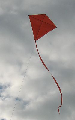


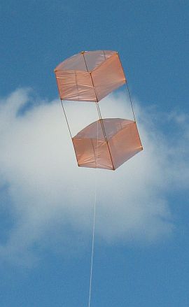


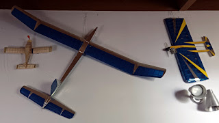
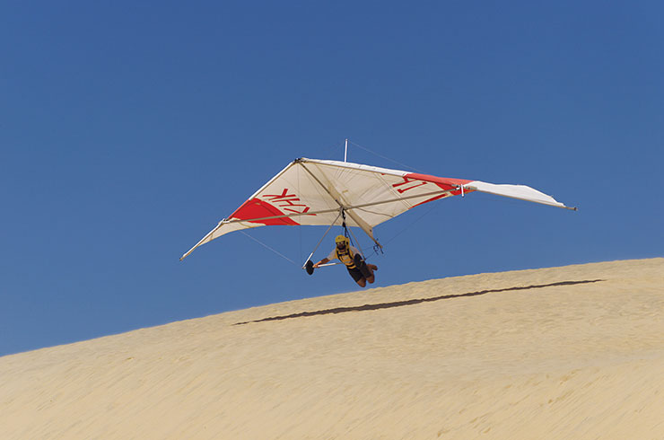 As a pre-teen, my family attended a party on a hilltop, from where a couple of hang glider pilots happened to be launching themselves. Pure flight. I was enthralled, even obsessed for a year or so. But it wasn't until my 30s that I could finally take one hang-gliding lesson, and that's as far as I got.


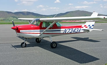

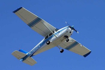
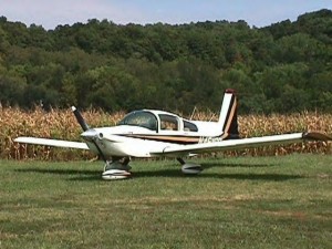
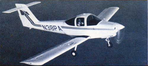
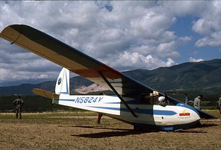

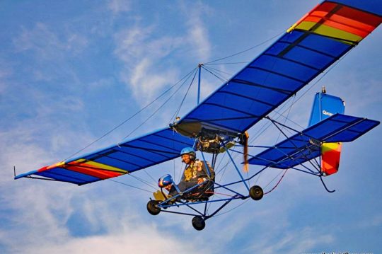
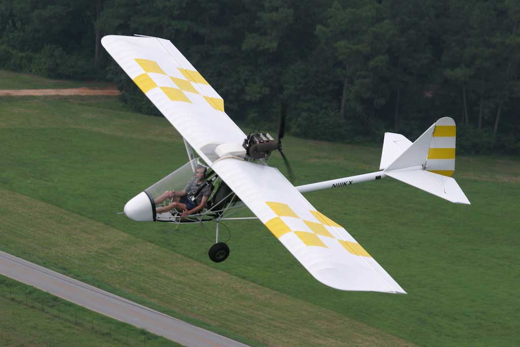
 Before I left Texas, a friend invited me skydiving. I did a tandem jump with an instructor strapped to my back. That first step into the void teaches you something about yourself that can't be easily described. I recommend the experience to anyone — but only once.
 The most difficult aircraft I ever flew was the MetLife blimp. It looks so slow and gentle, but blimps are hard to control and they respond only grudgingly. I could never fly it straight, but those MetLife blimp pilots could fly it through a narrow mountain pass with a 100 mph tail wind and land it on a dime. Those are hot pilots, in my view.
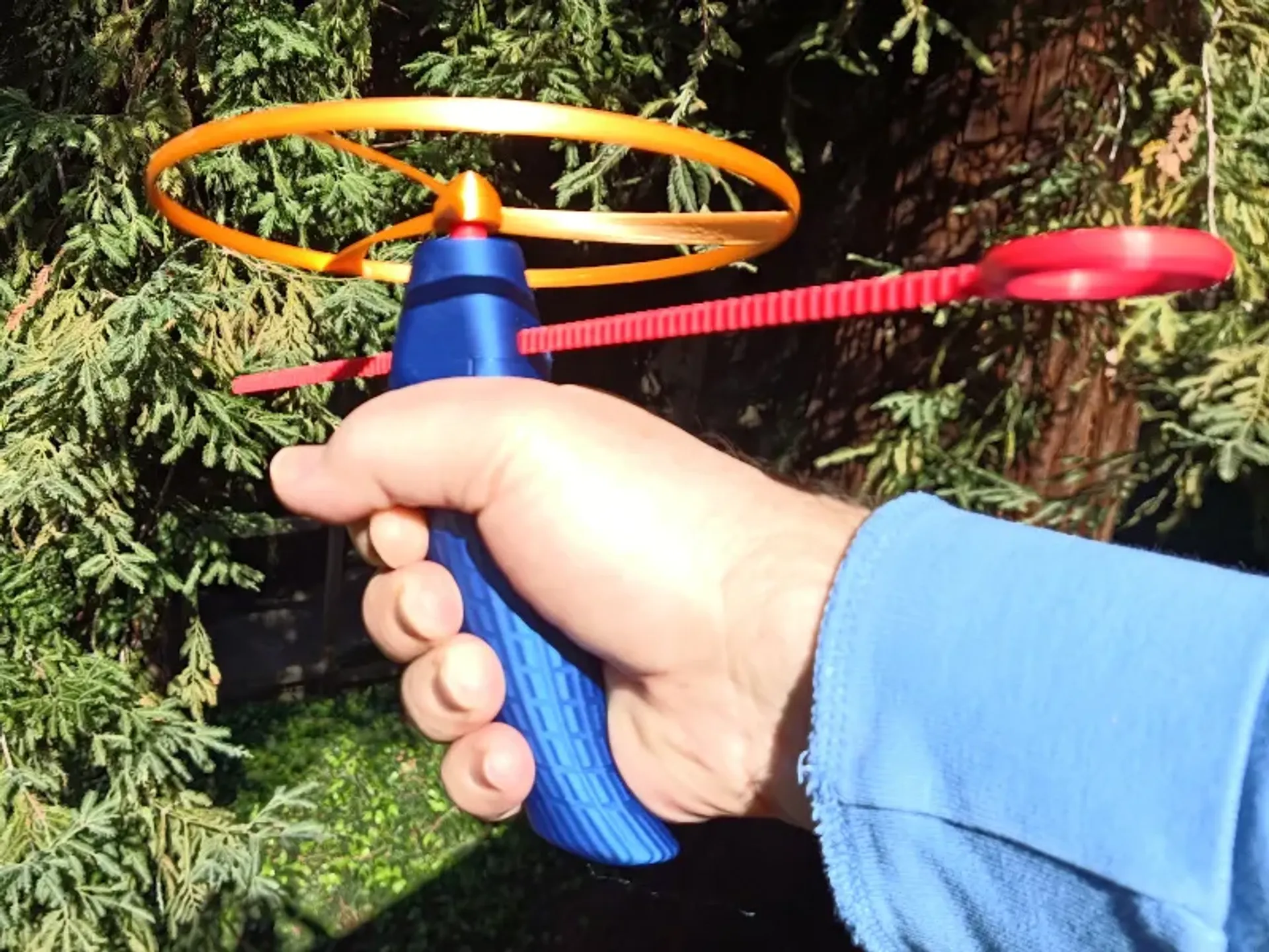
![[Spitfire]](https://upload.wikimedia.org/wikipedia/commons/thumb/4/4d/Spitfire_CGYQQ_Y2K_SN_TE294.jpg/330px-Spitfire_CGYQQ_Y2K_SN_TE294.jpg) You don't see aircraft with
You don't see aircraft with ![[Elliptical blade propeller]](https://blogger.googleusercontent.com/img/a/AVvXsEgFx__-ShmtRH7ouknOT9iT4NpBxMKg3NN2XjZOpKYqRGOVIjf5HSgrietupexlV8RnmZFOTpaCa8RKXDlx11BClP6t14EYU4hf3KhrCVpZO3VPwE46hziRFvkF_sUgjouBhfs4ougdc2O5dDh7mI1g9PPVEoxQIk_3KBEebcgklqmZf9doGI9aZcvg=s320)
![[Propeller with truncated ellipse blades]](https://blogger.googleusercontent.com/img/a/AVvXsEidOUA02gPi9-7f-DWly0X-d_Sg0ACwxHoo79V2LlldInBLItBKv8ffZ0O6e9vX3sS1e4WvZ29Rvg4WZjHcvnYtgd2UnKYrg7UKsJ2gdNdvbTJiBCqc-MMoFn7_h_GcjQxbJDZpD6cnS79-VfUfJbSBNM1DmTz-W_YfNdcQi8FIyKJoay_uGApPBsg0=s320)


![[Ergonomic handle dimension properties]](https://blogger.googleusercontent.com/img/a/AVvXsEhludIykX9vgF4_DphbH7FCTmakTSYysatMWn5e-UJqa1PGLP5Qp-9kvhwwmJSFO70o7aOf32dMg4SXpmDj14YFJf7Zh0cQr61tYdnDyZFcRwihhL3wIDwUBci-PvlGIN_5fP01828u8vrVLrOnT0ZJZMatxgoKy4I57ZyugIsGgeIuHBSeifftOUuT=s600)
![[CAD renderings of handles]](https://blogger.googleusercontent.com/img/a/AVvXsEjkaGDz6D9ahj2ScSZyz6NMTwiCnQGP_oZrSTTsJhU4B86fMe8FdhsRgqU3-ednZW-97reucn3zma9mD9BNtisdDNSIiEFZxQabwoTMkDB2n4VAvkTWqnWjBO6hJvh5wrMqIgg1iwx3fR6SExOTAkeFGeveLoNhRiZRTNCqjbnDCWIqICJh8cIYWCB5=s320)
![[handle too small for me]](https://blogger.googleusercontent.com/img/a/AVvXsEiOonCWtu1tzYFF9bEK1CedZKOnExnUW-qZwE9V4kHYKOJXQ0CRDYCXl-hSGV4lCkTK4swqpXWD5Zy432xxN0GEjUAsVQ20EENaqnTtE0FyqXdiwW5kecd3H3A0YL-BdOGJokWm_XZpSgYOjtnowT-Ct3bWUJtYHPfDJ-Zw6diTcQdtT2sCHXcGuq6G)
![[hand length and width]](https://blogger.googleusercontent.com/img/a/AVvXsEi-vK55Q-EGpBn_X7tyqjpgn_raL5AzedaNaBRM0AHcy3DDrCQ9UPdpTLh_bdeuJycfqs7HbPaovHiHgqka0pP_5hR9o5Wv8-ncWsw0K0fO-9ah3ZJ4Nl5G6ja51-czCqTKisKPpIyQ5LwwdLWedue_5TSd01mdVPzt4-xPOpsG4aidxkEGd7ktZb1K=s400)
![[comparison of control points]](https://blogger.googleusercontent.com/img/a/AVvXsEhKjQukozFzpU8OzMm6BST8OueQgJbIJ85J75Xe1dC-C392_9HGYZhaD6uzG5AJ18TdnJ5S3G6-D81wLk-gwVFhBaoNhVYEvzA-6tgFQDrl6DQ2-ePBEGfrNxJaOZd-vVQSpHTWmncS6HKwVeKtcjVN-M3LyClx1-C3UnBqUyiGafWOd4TSNxd-aPY2=s400)


![[Trochoid curve]](https://upload.wikimedia.org/wikipedia/commons/1/1c/TrohoidH0%2C8.gif)
![[Trochoid finger groove profile]](https://blogger.googleusercontent.com/img/b/R29vZ2xl/AVvXsEhWHdgUGpUJcrSUYFrObHkgbBczLmL9qeOaB4ItO0t-MnQIUqY3oJiBFiBjAmIrANeYwkJ9hW-MRZmVA50L5iyLam9lKH0wFs1am7WEI_xO_JB7r9pBy16N_fT-wpDUKb9T3KAt95AfbsYLTecEALfb627OBozjXEf19dtBVy-5Ln9CNID3X434yW0Z/s600/trochoid1.png)
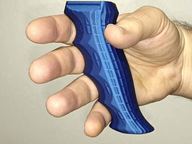


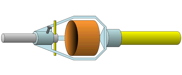
![[deck of cards]](https://blogger.googleusercontent.com/img/b/R29vZ2xl/AVvXsEib2OoH-Mu6zbD0jM_CCqRvYNnjlYb-9l83gdFcQdsV1OE1e8ZN9YsXW55PJscBBJ68eotb59jVEnbx9CDcgVPP9fPKtNCZ362OXRvmCUS7XIsbLRkEC_Xg9lkQaLJHTPB4jW3NoVLTW3g/s320/cards.jpg)


![[title image]](https://blogger.googleusercontent.com/img/b/R29vZ2xl/AVvXsEjwTnxnrSkI0zb_ba4W87yIFE0c65SB-sYRDbBl4QntWC5Okh-VzHuvsZ7YvUCxHdnxGt6BxW0KVm5E92IREnwKB-8BroxQ4_S7QbDTAScUKpsJjquNjbMReh_2QYai1R9jRatw3Jg0184/s1600/losing-weight.jpg)
![[fart blast]](https://blogger.googleusercontent.com/img/b/R29vZ2xl/AVvXsEgytcdk_lVUKR-6Pj8OeflXyXvmph3K1NZG_mZV7wClPxSNVmjgJfRM0Eegwrhje4DeJaJwDcCRvFGZnAAhgSRe_XZ75Cx2Tx9vlnqRgl19TnX9PNnBGXVU9CfPzK6XX88mo9p4AIkboQo/s1600/fartblast.jpg)
![[plate of sushi]](https://upload.wikimedia.org/wikipedia/commons/thumb/4/4c/Salmon_sushi_cut.jpg/320px-Salmon_sushi_cut.jpg)
![[fat frog]](https://upload.wikimedia.org/wikipedia/commons/thumb/3/3d/Fat_Frog_%286086664150%29.jpg/607px-Fat_Frog_%286086664150%29.jpg)
![[bowl of lettuce]](https://blogger.googleusercontent.com/img/b/R29vZ2xl/AVvXsEjIsoPq35NznyJ04hpQtnlfAa0sRNrWmWiyvbcQCgYegubVg46qL4udTeERn2GeM1JZX6gMwU6IxsC5Yb0CLkRGkA0SErsc7W1uTzElhvv-ZAJ0aTgmVkH3k6vVTQGx6QJtpO43nJiPcyc/s1600/salad02-lg.jpg)


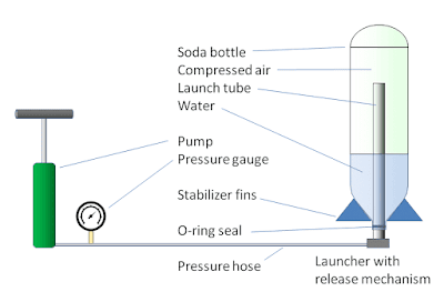
![[launching just the bottle]](https://upload.wikimedia.org/wikipedia/commons/1/11/WaterRocketLaunch.jpg)
![[images of launch sequence]](https://upload.wikimedia.org/wikipedia/commons/c/c0/Water_rocket_timing.jpg)