JabPerf Corp

Estimated reading time: 3 minutes

I’m going to tell you something that you probably already know. . . sequels usually suck. Oh, they got me when they told me that Denzel Washington would be in Gladiator II, that interminable dud of a film. How about that pitiful money-grab The Hangover II? And the “My Belly Laugh” differential between Bad Santa and Bad Santa 2 is probably the largest in my life as a moviegoer. And don’t even get me started on Joker: Folie à Deux – I don’t even wanna watch the *original* anymore after seeing that crap! But every now and then you get The Godfather II, a follow-up so sublime that I get almost as much enjoyment watching *others* experience it for the 1st time. Tech books follow a similar sequel trend, for the most part. But Performance Analysis & Tuning for Modern CPUs – Second Edition1 is The Godfather II of tech book sequels.

“What’s so great about this sequel, Mark?”

I’m glad you asked. Admittedly, the first edition was pretty Intel-heavy. But this time around, we made sure to incorporate more AMD-specific information, as well. Not only that, but we’ve included a completely different architecture – ARM. And if that weren’t enough, we fleshed out this sequel with comprehensive Case Studies and Hands-on exercises!

Also, while there were only a handful of us contributors for the first edition, we doubled that this time around. Along with Denis and myself, we added:

• Jan Wassenberg
• Swarup Sahoo
• Alois Kraus
• Marco Castorina
• Lally Singh
• University of Zaragoza, Spain

Dick Sites returned as a reviewer, and was accompanied this time around by the creator of every developers’ favorite online tool, Matt Godbolt of “Compiler Explorer” fame.2

“Will I be lost if I haven’t read the original?”

This is where “The Godfather” comparison begins to break down. I would never advise anyone to watch The Godfather II without having observed the Corleone family dynamic and Michael’s evolution in the original film. But that’s simply not the case with Performance Analysis & Tuning on Modern CPUs – Second Edition. This edition starts from the same base as the original and then expands upon it. We’ve updated/corrected issues in the first edition, buttressed each chapter with additional material, and even added new topics that are missing from the original – e.g., Continuous Profiling. In fact, you’re better off just reading the sequel if you never got around to reading the original.

A Sequel that Won’t Disappoint

You might be thinking, “Hey, Mark, why should I trust your word when you’re one of the Contributing Authors?” Good question. You shouldn’t trust *just* my word. Read the reviews from people like Dick Sites and Matt Godbolt. Or the verified reviews of Amazon customers. Then, after doing your due diligence, get one for yourself and for the techie family, friends, and colleagues in your life just in time for gift-giving this Holiday Season. Give them the gift of The Godfather II of tech books.

1    Paid affiliate link2    While Matt holds the crown for the illest last name in Tech, I remain at the top of the heap for best middle name, El Toro.

The post “The Godfather II” of Tech Book Sequels appeared first on JabPerf Corp.

Estimated reading time: 9 minutes

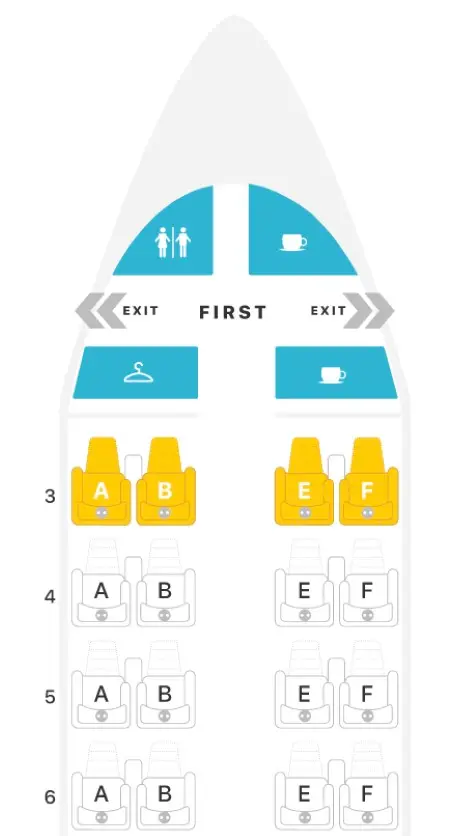
Sometimes, we run on autopilot when configuring CPU Affinity, turning over complete control to our intuition. It happens just as easily in everyday life, too. For example, while planning a vacation, a man buys adjacent airline seats for his family of four. He selects seats 3A, 3B, 3E, and 3F. “I got us the entire third row! Sweet!” Until he realizes too late that the more adjacent seating actually includes 3A, 3B, *4A* and *4B*.

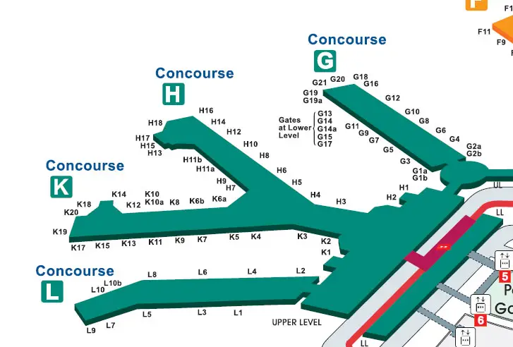
Then he notices that the connecting domestic flight at O’Hare will be at Gate H3. . . but they land at Gate K3! Sure, both gates are in the same terminal (Terminal 3), but they’re still in different concourses. He and his wife must race the kids & luggage from Concourse K all the way to Concourse H. But then as soon as they exit the plane to begin their track meet, he looks up to discover that Gate H3 is directly across from Gate K3. Crisis averted.

Intuitively, this guy imagined that choosing sequential seating within the same row gave him the best proximity. Then he figured an airport gate in Concourse H would be far from one in Concourse K. But his intuition failed him on both counts. Had he paid closer attention to the actual seating and terminal maps, he could’ve avoided this confusion.

The same is true with CPU Affinity. Everyone understands the benefits of CPU Affinity on NUMA systems. After all, who wants to endure cross-socket latency for CPU <=> RAM communication? But we’ve also become increasingly aware of nonuniformity on even *single* sockets, as evidenced by the recent proliferation of core-to-core latency measurement tools. Yet, how do many go about pinning application threads to cores? “Hmm, I’ll put this thread on core 1, this one on 2, and the last one on 3. Good, now they’re running as close together as possible.” Meanwhile, you pin the low priority threads faaaar away on core 23. That’s CPU Affinity on autopilot.

QUESTION: How much performance do we lose by configuring CPU Affinity for our multithreaded applications on autopilot?

Table of contents

• What Is CPU Affinity?
• Benefits of CPU Affinity
• Microarchitectural Evolution
• Microarchitecture Effects on CPU Affinity
• Demo
  • CPU Affinity: Cores 1 and 3
  • CPU Affinity: Cores 3 and 17
  • Results Analysis
• New Year’s Resolution: Thoughtful CPU Affinity

What Is CPU Affinity?

Firs things first – what exactly is CPU Affinity? It’s a technique that allows a user to assign (or pin) a process or thread to a specific compute resource or group of compute resources. By default, the OS schedules processes among all available cores using sophisticated heuristics to ensure a fair distribution of runtime. Employing CPU Affinity circumvents this scheduling decision process by pinning selected threads to a designated list of cores.

Benefits of CPU Affinity

Fairness is cool for general purpose computer usage. But when we want optimal performance, we don’t need the OS suddenly snatching our thread off its core only to later reschedule it on a completely different core, ruining any chance it had at achieving effective cache utilization. No, we don’t want fairness. We don’t want to wait in-line at the club. We want the bouncer to wave us to the front and walk us to our usual VIP table with our designated waitress. That’s right – no arbitrary switching of waitresses so that we’re forced to repeat our favorite drink order to rotating wait-staff all night.

That’s the benefit of CPU Affinity. No long run queue times. No thrashing of core caches due to rescheduling, forcing us to revisit LLC or RAM more often than necessary.

When it comes to multithreaded applications, we can ensure low latency inter-thread communication when we pin threads to adjacent cores. But how much lower could that latency go if we truly understood core adjacency on modern CPUs?

Microarchitectural Evolution

The days of the monolithic die are numbered. Enter the era of the chiplet, where smaller dies comprising a subset of cores and cache interconnect with other such dies on a single CPU. Oh sure, Intel held out for as long as it could. But with the slowing of Moore’s Law and the breakdown in Dennard Scaling, Intel finally capitulated with the adoption of Embedded Multi-Die Interconnect Bridge (EMIB) interconnect technology for the higher core count Sapphire Rapids variants. AMD joined the chiplet movement much earlier with its Infinity Fabric interconnect via which multiple Core Complex Dies (CCDs), each housing one or more Core Complexes (CCXs), communicate through an IO Die (IOD).

Heck, there’s even the recent Universal Chiplet Interconnect Express (UCIe) open specification for chiplet interconnect to which Intel, AMD, ARM, and several others belong. Yep, you read that right – a standard that paves the way to mix & match plug-and-play chiplets!

This chiplet momentum brings the latency implications of multi-socket NUMA systems down to the level of a single socket. Why? Because the chiplets on modern CPUs are essentially sockets unto themselves, with AMD’s Infinity Fabric and Intel’s EMIB standing in as the inter-socket connection (e.g., HyperTransport or UPI).

So, how should this affect how we perform CPU Affinity?

Microarchitecture Effects on CPU Affinity

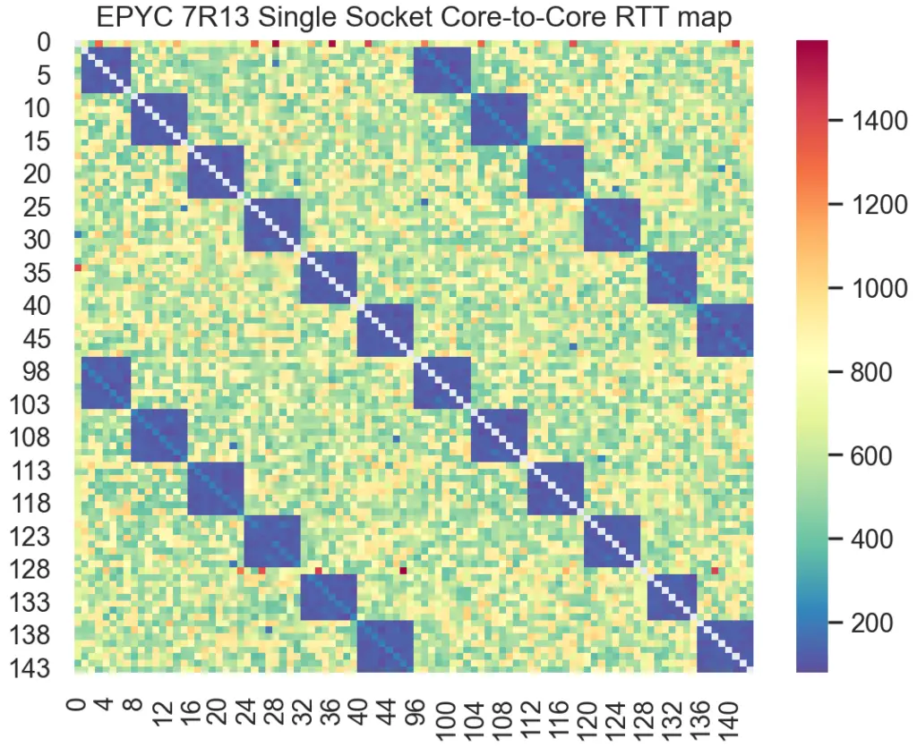
Naturally, the cores that reside within the same chiplet exhibit lower communication latency than that between cores in disparate chiplets. Pick up any one of the several available core-to-core latency measurement tools and run it on your own CPU for proof.

For example, here’s the latency heatmap produced from one such tool on AMD’s Milan. Notice the deep blue blocks clearly highlighting the lowest latency for cores within the same CCD:

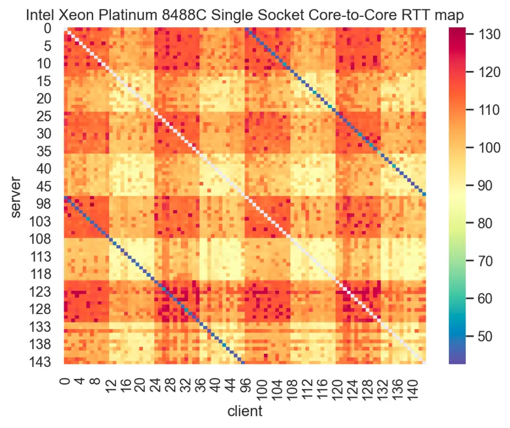
Here’s another heatmap from the same tool used on Intel’s Sapphire Rapids:

Notice the wide range in inter-core communication latency across a single socket for both Milan and Sapphire Rapids. Now, think back to a time when you pinned threads to cores on the same socket, each core number selected sequentially, confident that this sufficed to indicate location. How much performance did you leave on the table doing that?

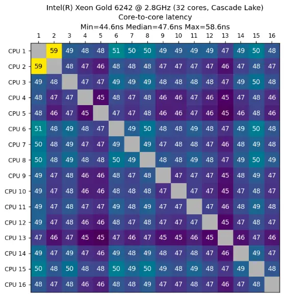
And this is not just some recent phenomenon, by the way. Such CPU nonuniformity actually predates this chiplet era. For example, take a look at this latency heatmap from an Intel Cascade Lake, taken using a different core-to-core latency measurement tool:

Cascade Lake uses a *monolithic* die. Yet, notice the spread in inter-core latency – a minimum of 44.6ns and a maximum of 58.6ns. That’s a 14ns spread on a single die comprising only 16 cores. Now extrapolate that to a chiplet-based CPU with a factor of 3x or more cores! That really adds up over the total runtime of a multithreaded application.

But how much does it add up to, really? Let’s test it out.

NOTE: For an in-depth discussion on CPU microarchitecture and squeezing the most performance from it, check out our book Performance Analysis and Tuning on Modern CPUs.1

Demo

Our demo uses an Intel Sapphire Rapids-based system comprising 16 cores running Rocky 8.6. We isolate all cores of the 2nd socket (all odd-numbered cores) from the kernel scheduler using the isolcpus boot parameter to minimize interference:

[mdawson@eltoro ~]$ lscpu
Architecture:        x86_64
CPU op-mode(s):      32-bit, 64-bit
Byte Order:          Little Endian
CPU(s):              32
On-line CPU(s) list: 0-31
Thread(s) per core:  1
Core(s) per socket:  16
Socket(s):           2
NUMA node(s):        2
Vendor ID:           GenuineIntel
CPU family:          6
Model:               143
Model name:          Intel(R) Xeon(R) Gold 6444Y
Stepping:            8
CPU MHz:             4000.000
BogoMIPS:            7200.00
L1d cache:           48K
L1i cache:           32K
L2 cache:            2048K
L3 cache:            46080K
NUMA node0 CPU(s):   0,2,4,6,8,10,12,14,16,18,20,22,24,26,28,30
NUMA node1 CPU(s):   1,3,5,7,9,11,13,15,17,19,21,23,25,27,29,31

[mdawson@eltoro ~]$ lscpu
Architecture:        x86_64
CPU op-mode(s):      32-bit, 64-bit
Byte Order:          Little Endian
CPU(s):              32
On-line CPU(s) list: 0-31
Thread(s) per core:  1
Core(s) per socket:  16
Socket(s):           2
NUMA node(s):        2
Vendor ID:           GenuineIntel
CPU family:          6
Model:               143
Model name:          Intel(R) Xeon(R) Gold 6444Y
Stepping:            8
CPU MHz:             4000.000
BogoMIPS:            7200.00
L1d cache:           48K
L1i cache:           32K
L2 cache:            2048K
L3 cache:            46080K
NUMA node0 CPU(s):   0,2,4,6,8,10,12,14,16,18,20,22,24,26,28,30
NUMA node1 CPU(s):   1,3,5,7,9,11,13,15,17,19,21,23,25,27,29,31

We’ll use our own adaptation of Martin Thompson’s InterThreadLatency code to benchmark transfer rate between a thread pair while varying only its CPU affinity. Our version of the benchmark is called simply ping-pong.

The test exchanges two messages serially, each one updated by only one of the threads, for a fixed number of iterations. The output is a transfer rate in “op/sec”, and we take the harmonic mean of 30 samples for each affinity scenario. Since we practice “Active Benchmarking” here at JabPerf, we will run each scenario under perf stat -d to obtain metrics during execution; otherwise, we’re just as negligent as those other clickbait benchmark articles.

#include <time.h>
#include <pthread.h>
#include <stdio.h>
#include <stdlib.h>
#include <stdint.h>
#include <sched.h>
#include <unistd.h>

const uint64_t ITERATIONS = 500LL * 1000LL * 1000LL;

volatile uint64_t s1 = 0;
volatile uint64_t s2 = 0;

void* run(void*)
{
    register uint64_t value = s2;
    while (true)
    {
        while (value == s1)
        {
            // busy spin
        }
        value = __sync_add_and_fetch(&s2, 1);
    }
}

int main (int argc, char *argv[])
{
    if(argc < 3)
    {
        puts("Please specify the server and client core numbers");
        return(-1);
    }

    auto server_core = atoi(argv[1]);
    auto client_core = atoi(argv[2]);

    cpu_set_t cpu_set_server, cpu_set_client;
    CPU_ZERO(&cpu_set_server);
    CPU_ZERO(&cpu_set_client);
    CPU_SET(server_core, &cpu_set_server);
    CPU_SET(client_core, &cpu_set_client);

    sched_setaffinity(getpid(), sizeof(cpu_set_server), &cpu_set_server);

    pthread_t thread;
    pthread_create(&thread, NULL, run, NULL);
    pthread_setaffinity_np(thread, sizeof(cpu_set_client), &cpu_set_client);

    timespec ts_start;
    timespec ts_finish;
    clock_gettime(CLOCK_MONOTONIC, &ts_start);

    register uint64_t value = s1;
    while (s1 < ITERATIONS)
    {
        while (s2 ! = value)
        {
            // busy spin
        }
        value = __sync_add_and_fetch(&s1, 1);
    }

    clock_gettime(CLOCK_MONOTONIC, &ts_finish);

    uint64_t start = (ts_start.tv_sec * 1000000000LL) + ts_start.tv_nsec;
    uint64_t finish = (ts_finish.tv_sec * 1000000000LL) + ts_finish.tv_nsec;
    uint64_t duration = finish - start;

    printf("duration = %lldn", duration);
    printf("ns per op = %lldn", (duration / (ITERATIONS * 2)));
    printf("op/sec = %lldn",
        ((ITERATIONS * 2L * 1000L * 1000L * 1000L) / duration));
    printf("s1 = %lld, s2 = %lldn", s1, s2);

    return 0;
}

#include <time.h>
#include <pthread.h>
#include <stdio.h>
#include <stdlib.h>
#include <stdint.h>
#include <sched.h>
#include <unistd.h>

const uint64_t ITERATIONS = 500LL * 1000LL * 1000LL;

volatile uint64_t s1 = 0;
volatile uint64_t s2 = 0;

void* run(void*)
{
    register uint64_t value = s2;
    while (true)
    {
        while (value == s1)
        {
            // busy spin
        }
        value = __sync_add_and_fetch(&s2, 1);
    }
}

int main (int argc, char *argv[])
{
    if(argc < 3)
    {
        puts("Please specify the server and client core numbers");
        return(-1);
    }

    auto server_core = atoi(argv[1]);
    auto client_core = atoi(argv[2]);

    cpu_set_t cpu_set_server, cpu_set_client;
    CPU_ZERO(&cpu_set_server);
    CPU_ZERO(&cpu_set_client);
    CPU_SET(server_core, &cpu_set_server);
    CPU_SET(client_core, &cpu_set_client);

    sched_setaffinity(getpid(), sizeof(cpu_set_server), &cpu_set_server);

    pthread_t thread;
    pthread_create(&thread, NULL, run, NULL);
    pthread_setaffinity_np(thread, sizeof(cpu_set_client), &cpu_set_client);

    timespec ts_start;
    timespec ts_finish;
    clock_gettime(CLOCK_MONOTONIC, &ts_start);

    register uint64_t value = s1;
    while (s1 < ITERATIONS)
    {
        while (s2 ! = value)
        {
            // busy spin
        }
        value = __sync_add_and_fetch(&s1, 1);
    }

    clock_gettime(CLOCK_MONOTONIC, &ts_finish);

    uint64_t start = (ts_start.tv_sec * 1000000000LL) + ts_start.tv_nsec;
    uint64_t finish = (ts_finish.tv_sec * 1000000000LL) + ts_finish.tv_nsec;
    uint64_t duration = finish - start;

    printf("duration = %lldn", duration);
    printf("ns per op = %lldn", (duration / (ITERATIONS * 2)));
    printf("op/sec = %lldn",
        ((ITERATIONS * 2L * 1000L * 1000L * 1000L) / duration));
    printf("s1 = %lld, s2 = %lldn", s1, s2);

    return 0;
}

Without further ado, let’s start the show!

CPU Affinity: Cores 1 and 3

The first affinity test represents the “autopilot” method, wherein sequential core numbering provides “enough” intuitive evidence of proximity:

[mdawson@eltoro ~]$ perf stat -d -r 30 ./ping-pong 1 3 --post sleep 5

 Performance counter stats for './ping-pong 1 3 --post sleep 5' (30 runs):

        123,347.69 msec task-clock                #    1.915 CPUs utilized            ( +-  1.32% )
                 3      context-switches          #    0.023 /sec                     ( +-  3.43% )
                 2      cpu-migrations            #    0.016 /sec
               114      page-faults               #    0.885 /sec
   492,329,584,771      cycles                    #    3.821 GHz                      ( +-  1.32% )
   116,256,410,619      instructions              #    0.23  insn per cycle           ( +-  1.16% )
    37,756,258,410      branches                  #  293.023 M/sec                    ( +-  1.19% )
     1,140,381,441      branch-misses             #    3.02% of all branches          ( +-  0.61% )
 2,953,977,508,626      slots                     #   22.926 G/sec                    ( +-  1.32% )
    98,465,578,134      topdown-retiring          #      3.1% retiring                ( +-  1.15% )
   295,398,315,560      topdown-bad-spec          #      9.6% bad speculation         ( +-  0.52% )
   648,716,629,344      topdown-fe-bound          #     20.9% frontend bound          ( +-  0.31% )
 1,922,981,211,108      topdown-be-bound          #     66.4% backend bound           ( +-  1.98% )
    17,376,451,225      topdown-heavy-ops         #      0.5% heavy operations       #      2.6% light operations        ( +-  2.44% )
   214,308,511,013      topdown-br-mispredict     #      7.0% branch mispredict      #      2.6% machine clears          ( +-  0.73% )
   115,842,706,999      topdown-fetch-lat         #      3.6% fetch latency          #     17.3% fetch bandwidth         ( +-  1.01% )
 1,755,009,602,189      topdown-mem-bound         #     61.1% memory bound           #      5.4% Core bound              ( +-  2.10% )
    38,749,344,790      L1-dcache-loads           #  300.730 M/sec                    ( +-  1.16% )
     1,093,477,009      L1-dcache-load-misses     #    2.82% of all L1-dcache accesses  ( +-  1.63% )
     1,093,453,003      LLC-loads                 #    8.486 M/sec                    ( +-  1.63% )
             2,259      LLC-load-misses           #    0.00% of all LL-cache accesses  ( +-  4.87% )

            64.427 +- 0.815 seconds time elapsed  ( +-  1.27% )

[mdawson@eltoro ~]$ perf stat -d -r 30 ./ping-pong 1 3 --post sleep 5

 Performance counter stats for './ping-pong 1 3 --post sleep 5' (30 runs):

        123,347.69 msec task-clock                #    1.915 CPUs utilized            ( +-  1.32% )
                 3      context-switches          #    0.023 /sec                     ( +-  3.43% )
                 2      cpu-migrations            #    0.016 /sec
               114      page-faults               #    0.885 /sec
   492,329,584,771      cycles                    #    3.821 GHz                      ( +-  1.32% )
   116,256,410,619      instructions              #    0.23  insn per cycle           ( +-  1.16% )
    37,756,258,410      branches                  #  293.023 M/sec                    ( +-  1.19% )
     1,140,381,441      branch-misses             #    3.02% of all branches          ( +-  0.61% )
 2,953,977,508,626      slots                     #   22.926 G/sec                    ( +-  1.32% )
    98,465,578,134      topdown-retiring          #      3.1% retiring                ( +-  1.15% )
   295,398,315,560      topdown-bad-spec          #      9.6% bad speculation         ( +-  0.52% )
   648,716,629,344      topdown-fe-bound          #     20.9% frontend bound          ( +-  0.31% )
 1,922,981,211,108      topdown-be-bound          #     66.4% backend bound           ( +-  1.98% )
    17,376,451,225      topdown-heavy-ops         #      0.5% heavy operations       #      2.6% light operations        ( +-  2.44% )
   214,308,511,013      topdown-br-mispredict     #      7.0% branch mispredict      #      2.6% machine clears          ( +-  0.73% )
   115,842,706,999      topdown-fetch-lat         #      3.6% fetch latency          #     17.3% fetch bandwidth         ( +-  1.01% )
 1,755,009,602,189      topdown-mem-bound         #     61.1% memory bound           #      5.4% Core bound              ( +-  2.10% )
    38,749,344,790      L1-dcache-loads           #  300.730 M/sec                    ( +-  1.16% )
     1,093,477,009      L1-dcache-load-misses     #    2.82% of all L1-dcache accesses  ( +-  1.63% )
     1,093,453,003      LLC-loads                 #    8.486 M/sec                    ( +-  1.63% )
             2,259      LLC-load-misses           #    0.00% of all LL-cache accesses  ( +-  4.87% )

            64.427 +- 0.815 seconds time elapsed  ( +-  1.27% )

CPU Affinity: Cores 3 and 17

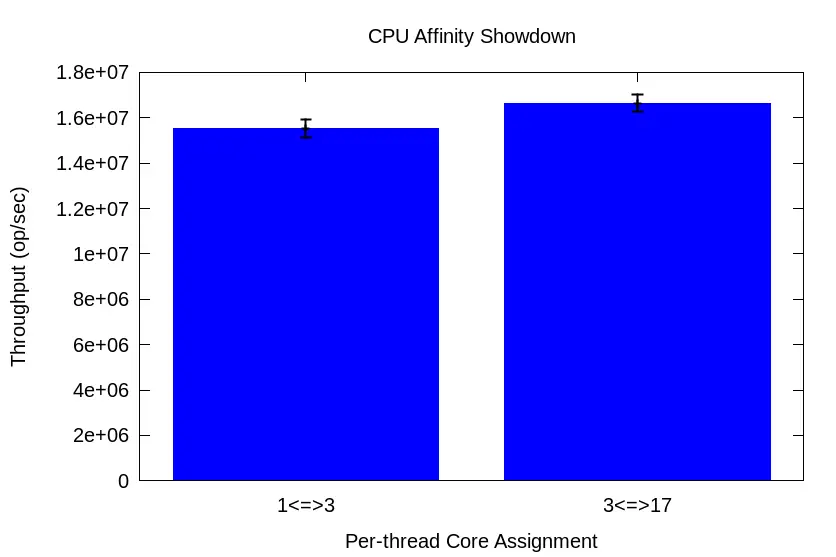
The second affinity test represents a more deliberate method of CPU Affinity, using information from a core-to-core latency measurement tool as the basis for selecting adjacent cores:

[mdawson@eltoro ~]$ perf stat -d -r 30 ./ping-pong 3 17 --post sleep 5

 Performance counter stats for './ping-pong 3 17 --post sleep 5' (30 runs):

        115,453.25 msec task-clock                #    1.922 CPUs utilized            ( +-  1.14% )
                 3      context-switches          #    0.025 /sec                     ( +-  3.48% )
                 2      cpu-migrations            #    0.017 /sec
               114      page-faults               #    0.949 /sec
   460,816,877,399      cycles                    #    3.835 GHz                      ( +-  1.14% )
   116,594,571,811      instructions              #    0.24  insn per cycle           ( +-  1.61% )
    37,866,504,741      branches                  #  315.152 M/sec                    ( +-  1.65% )
     1,152,422,965      branch-misses             #    3.18% of all branches          ( +-  0.59% )
 2,764,901,264,394      slots                     #   23.011 G/sec                    ( +-  1.14% )
    97,584,784,218      topdown-retiring          #      3.2% retiring                ( +-  1.22% )
   287,332,834,357      topdown-bad-spec          #      9.9% bad speculation         ( +-  0.58% )
   628,879,520,128      topdown-fe-bound          #     21.7% frontend bound          ( +-  0.62% )
 1,756,525,509,143      topdown-be-bound          #     65.1% backend bound           ( +-  1.55% )
    16,264,116,656      topdown-heavy-ops         #      0.6% heavy operations       #      2.6% light operations        ( +-  2.50% )
   216,854,967,417      topdown-br-mispredict     #      7.2% branch mispredict      #      2.7% machine clears          ( +-  0.55% )
   108,427,466,853      topdown-fetch-lat         #      3.8% fetch latency          #     18.0% fetch bandwidth         ( +-  0.85% )
 1,604,727,042,064      topdown-mem-bound         #     59.7% memory bound           #      5.4% Core bound              ( +-  1.64% )
    38,863,301,146      L1-dcache-loads           #  323.448 M/sec                    ( +-  1.61% )
     1,075,108,857      L1-dcache-load-misses     #    2.89% of all L1-dcache accesses  ( +-  0.98% )
     1,075,084,908      LLC-loads                 #    8.948 M/sec                    ( +-  0.98% )
             1,995      LLC-load-misses           #    0.00% of all LL-cache accesses  ( +-  4.21% )

            60.078 +- 0.660 seconds time elapsed  ( +-  1.10% )

[mdawson@eltoro ~]$ perf stat -d -r 30 ./ping-pong 3 17 --post sleep 5

 Performance counter stats for './ping-pong 3 17 --post sleep 5' (30 runs):

        115,453.25 msec task-clock                #    1.922 CPUs utilized            ( +-  1.14% )
                 3      context-switches          #    0.025 /sec                     ( +-  3.48% )
                 2      cpu-migrations            #    0.017 /sec
               114      page-faults               #    0.949 /sec
   460,816,877,399      cycles                    #    3.835 GHz                      ( +-  1.14% )
   116,594,571,811      instructions              #    0.24  insn per cycle           ( +-  1.61% )
    37,866,504,741      branches                  #  315.152 M/sec                    ( +-  1.65% )
     1,152,422,965      branch-misses             #    3.18% of all branches          ( +-  0.59% )
 2,764,901,264,394      slots                     #   23.011 G/sec                    ( +-  1.14% )
    97,584,784,218      topdown-retiring          #      3.2% retiring                ( +-  1.22% )
   287,332,834,357      topdown-bad-spec          #      9.9% bad speculation         ( +-  0.58% )
   628,879,520,128      topdown-fe-bound          #     21.7% frontend bound          ( +-  0.62% )
 1,756,525,509,143      topdown-be-bound          #     65.1% backend bound           ( +-  1.55% )
    16,264,116,656      topdown-heavy-ops         #      0.6% heavy operations       #      2.6% light operations        ( +-  2.50% )
   216,854,967,417      topdown-br-mispredict     #      7.2% branch mispredict      #      2.7% machine clears          ( +-  0.55% )
   108,427,466,853      topdown-fetch-lat         #      3.8% fetch latency          #     18.0% fetch bandwidth         ( +-  0.85% )
 1,604,727,042,064      topdown-mem-bound         #     59.7% memory bound           #      5.4% Core bound              ( +-  1.64% )
    38,863,301,146      L1-dcache-loads           #  323.448 M/sec                    ( +-  1.61% )
     1,075,108,857      L1-dcache-load-misses     #    2.89% of all L1-dcache accesses  ( +-  0.98% )
     1,075,084,908      LLC-loads                 #    8.948 M/sec                    ( +-  0.98% )
             1,995      LLC-load-misses           #    0.00% of all LL-cache accesses  ( +-  4.21% )

            60.078 +- 0.660 seconds time elapsed  ( +-  1.10% )

Results Analysis

As we’d expect, most of the CPU metrics roughly match since it’s the exact same code. However, notice the far fewer cycles and slightly higher IPC for the 3 <=> 17 affinity config vs. that of the 1 <=> 3 config. Not only that, but the L1d throughput rate is ~23MB/s higher, as well. When cores wait less time for memory transfers, they can get back to work more quickly.

“But how can this be when cores 1 and 3 are so close together, while core 17 is waaay over there?” It’s because our intuition about sequential core numbering hinders us from employing effective CPU Affinity.

How does all this translate into ping-pong transfer rates?

Across 30 runs, harmonic mean transfer rate for the 1<=>3 test is 15,521,920 op/sec with a 95% CI of 15,130,333 to 15,934,314. But for the 3<=>17 test, the harmonic mean transfer rate is 16,645,518 op/sec with a *narrower* 95% CI of 16,279,917 to 17,027,917. That’s a 7% boost in throughput w/o a single code change! That’s the kind of boost you’d expect after dealing with the multiple compilations and representative workload maintenance necessary for profile-guided optimization (PGO)!

And remember, this is a monolithic 16-core CPU. How much wider of a performance disparity would we discover across core pairs on a 40-, 60-, or 90-core chiplet-based CPU?

New Year’s Resolution: Thoughtful CPU Affinity

Let’s face it. If you truly care about low latency and/or high throughput, there’s a standard list of things you’re gonna do. Among them will include:

• Side-stepping the OS scheduler with CPU Affinity for a thread-per-core configuration
• Avoiding direct data sharing and the synchronization overhead (i.e., locking) it requires by utilizing message-passing between application threads

If this describes you, then it behooves you to pay closer attention to the way you pin threads to cores. I’ve observed 5 – 10% performance improvements in real-world applications, and I wouldn’t be surprised to find even greater improvements on higher core count CPUs.

Make it your 2024 New Year’s Resolution. And believe me, this will require MUCH less work and FAR less time commitment than your other resolution (and you know good & well which resolution of yours I’m talkin’ about).

1    Paid affiliate link

The post CPU Affinity: Because Even A Single Chip Is Nonuniform appeared first on JabPerf Corp.

Estimated reading time: 13 minutes

“If you’re thinking about buying a book, just buy it. Don’t waste five seconds debating it. Even one idea makes it more than worth the price.”

Ramit Sethi

Among the most frequently submitted questions I get from IT professionals and recent CS grads alike is: ‘What books would you recommend for anyone interested in performance?’ In fact, I’ve answered that question enough to warrant this dedicated blog post. And I’m especially qualified to answer it given my lifelong adherence to Ramit’s aforementioned advice. Oh, I’ve bought all sorts of tech books ranging widely in price and content quality. Many were duds. Some light on depth (e.g., glorified man pages). Others light on facts, believe it or not. But every now & then I’d stumble upon a goldmine. Even among a lot of the duds sprung an occasional leak of insight which led me to a breakthrough.

It was a long trudge to reach this point. But to quote the preeminent wordsmith Shawn Carter a.k.a. Jay-Z, “Hov did that, so hopefully you won’t have to go through that.” So, by all means, benefit from the fruits of my labor as I present you my personal Top 7 list of performance books for engineers.1

Table of contents

• Book Selection Criteria
• My Top 7 Performance Books for Engineers
  • 1. The Every Computer Performance Book
  • 2. Analyzing Computer Performance with Perl::PDQ
  • 3. Understanding Software Dynamics
  • 4. Systems Performance: Enterprise and the Cloud
  • 5. Pro .NET Benchmarking
  • 6. The Art of Writing Efficient Programs
  • 7. Troubleshooting with Wireshark
• Further Reading

Book Selection Criteria

I already know what you’re thinking. ‘He’s just gonna plug the book that he helped work on for Denis Bahkvalov.’ No, no, no, that’s not gonna happen at all. Nor will I attempt to plug the second edition of the aforementioned work, either. While I firmly believe those are great additions to any engineer’s introduction to the beautiful art & science of Software Performance, I purposely left them off the list. There’s no room for personal bias on this blog.

Also, I’ve left off performance books published more than 15 years ago despite the impact they may’ve exerted on engineers and authors of subsequent works. If not for this somewhat arbitrary cutoff point, more Adrian Cockroft, Richard McDougall, and Jim Mauro references would appear here.

My Top 7 Performance Books for Engineers

This is NOT an exhaustive list of every good performance book I’ve ever read. This is only a list of the ones I most often recommend to technologists from other disciplines who express an interest in the area of performance analysis & engineering.

NOTE: Each book image is a clickable link.

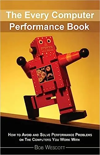
1. The Every Computer Performance Book

When I first learned to box as a kid, I was excited to learn all the dazzling punch combos. But what did my coach teach me in my first lesson? Proper stance. After that? How to step forward & back. Then? How to step right & left. I don’t even remember when I actually threw my first punch! But a firm grasp of proper footwork and balance paved the way for eventually learning effective punch combos. No matter what new skillsets I picked up later on, my footwork *always* served me well for incorporating them.

It’s similar in software performance. Overeager techies wanna tinker with magic knobs & secret tunables hidden behind names with leading underscores. They want the tricks of the trade w/o first understanding the trade itself. But that’s not Performance Engineering, and those tweaks only pertain to specific software packages and versions. It’s the transferable concepts and skills which retired Performance Consultant Bob Wescott shares in his swan song.

It’s a short & witty, yet dense distillation of key concepts that will serve you well throughout your career. He could’ve rattled off nitty-gritty details of Queuing Theory, or all the technology-specific knobs he picked up along the way. Instead, Bob homes in on the essentials he most commonly encountered across engagements. That’s where this book shines. It brims with hard-earned experience instead of ethereal mumbo-jumbo or urban legends handed down from Usenet groups of yore.

And his book runs the gamut from Monitoring & Modeling to Capacity Planning & Load Testing. He even schools us on handling political issues that arise when presenting performance analyses. Yep, pesky little facts can potentially land us in hot water, even in cases where the boss requests them! At only ~200 pages, it’s a quick yet engaging & informative read for any engineer aspiring to enter this space.

2. Analyzing Computer Performance with Perl::PDQ

My point in recommending this book is not to push his Perl::PDQ tool (it’s also available in C, Python, and R these days). It’s all the foundational performance principles the author establishes leading up to the tool’s introduction that earns its spot on the list. The author I’m referring to is none other than Neil Gunther, father of Universal Scalability Law (USL). Where Wescott’s book gives us the gist of Queuing Theory, Gunther dives fully into the subject.

But this is not some academic book full of formulas but woefully lacking in real-world application. On the contrary, he cogently illustrates just how useful Queuing Theory is with ample, concrete examples (e.g., multicore/multiprocessor architectures, multi-tier web apps, virtual machine configs, benchmark analysis, etc.). You walk away understanding that anything can be modeled as a queue or network of queues and, therefore, can be reasoned about using these laws. His handy PDQ tool just makes them much easier to wield. It’s truly a remarkable performance book, and I can’t recommend it enough.

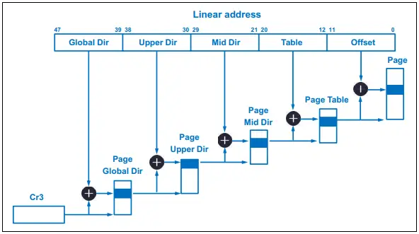
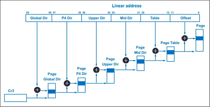
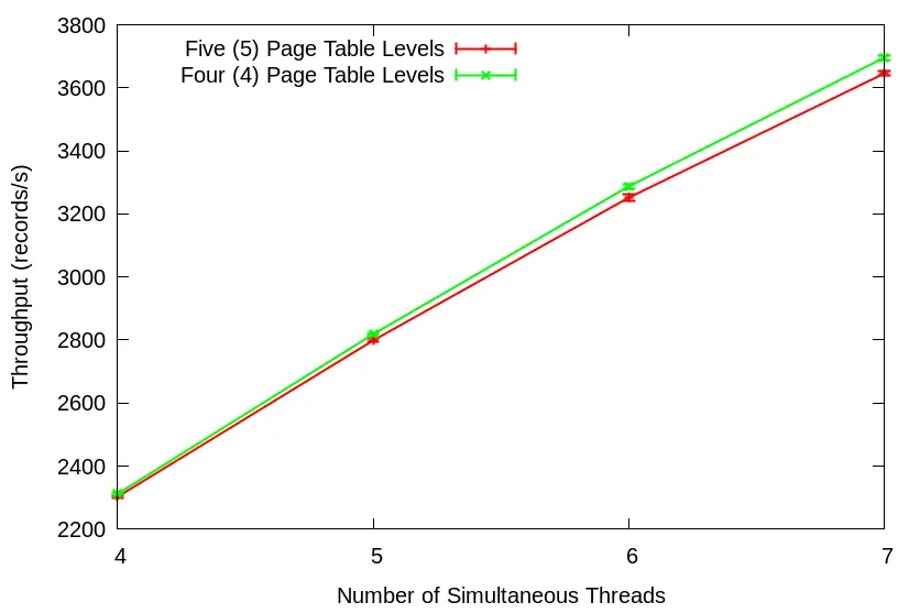
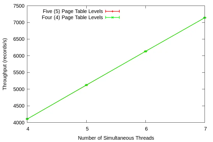
On a side note, Neil is still active on Twitter. He once used the graphs from my “5-level vs. 4-level Page Tables” article & calculated the alpha coefficient (i.e., the Contention factor in the USL model) imposed by 5-level kernel page tables for my Twitter followers. I thought that was pretty cool. By the way, USL packages are available in Python and R.

3. Understanding Software Dynamics

No other performance book evokes the mentor-mentee relationship in literary form more than this post-retirement entry (the 2nd retiree on this list) from the venerable Dick Sites. It teems with realistic examples and Case Studies which impart his wisdom gained through decades in the trenches.

The book offers a framework for reasoning about tail latency in complex software systems. He shows how building a mental model for how long things *should* take, within an order of magnitude, is essential to this framework. Without such an understanding, how can you recognize anomalous behavior that requires investigation? And it’s in this first section where many software developers will benefit most as he lays out that mental model. There he describes the performance behavior of the 5 fundamental resources: CPU, Memory, Disk/SSD, Network, and Software Critical Section. For a generation of CompSci grads entering the workforce knowledgeable in Frameworks & Design Patterns w/o even the slightest idea of how code interacts with underlying HW, this first section should be required reading.

Yet, this performance book offers much more. It covers tooling and effective methods of observing software<->hardware interplay that provide valuable clues for tail latency investigation. Finally, it wraps up with a section on reasoning from the observational data we’ve obtained. This final section comprises the aforementioned Case Studies that build upon everything laid out in the previous sections.

Because this book addresses topics at a lower level than the previous two on this list, the author had to settle upon a few technologies from which to pull examples. He chose C/C++ and Linux running on Intel, AMD, and ARM CPUs. But the lessons & principles transfer well across any technology stack. I only wish this book was available when I first entered the workforce.

4. Systems Performance: Enterprise and the Cloud

Y’all saw this one comin’ from a mile away, didn’t ya? This is Brendan Gregg’s 2nd edition, and is a performance book that works primarily from the Linux OS/kernel perspective, with comprehensive coverage of cloud technologies added. While it covers the performance characteristics and observability tools for the same 5 computing resources covered in Dick’s book, Brendan’s dives quite a bit deeper given its OS-level theme. Another difference between their books is the breadth of coverage on the idiosyncrasies of VM/Container performance analysis, whether on-prem or in the cloud.

While the aforementioned points would be enough to warrant a spot on my list, the book goes further by outlining and ranking commonly used methodologies of Performance Analysis and Benchmarking. Regarding the latter, I believe the industry as a whole will benefit from reading and revisiting on a monthly basis section 12 on Benchmarking. Anyone who has ever read my blog will understand why I say this. Lastly, all software developers should print out & frame a copy of the “7 Performance Mantras” from section 2.5.20. I know several software engineers who have done so already.

At over 800 pages, this book is a comprehensive treatment of Performance Engineering for the modern, cloud-native age. My guess is that you already have it in your library, but this list would lack credibility w/o it.

5. Pro .NET Benchmarking

Hands down, this is the best benchmarking book I’ve ever read. There, I said it. “But, but, but. . . it’s about .NET.” No, it simply uses .NET for illustrative purposes but all concepts and takeaways are largely transferable.

Look, I’ve read many performance books for engineers that dedicated a chapter or even an entire section to the topic of Benchmarking (See previous heading). And the quality of handling of the topic varied widely in those publications. But, other than a couple of huge academic tomes filled with more formulas than sentences, this is the only *practical* book entirely devoted to a competent coverage of the subject. Best practices, gotchas, measurement bias, proper analysis, tooling, etc. I particularly like that he stresses the importance of visualizing runtime distributions – performance is a shape, not a number.

But what I love most about Andrey’s book is the chapter he devotes to Statistics. As a Performance Engineer, you absolutely CANNOT offer much benefit to customers w/o a solid grasp of Statistics. But who wants to study any of those 900-page, inscrutable volumes on the topic?! I certainly didn’t want to. So, I absorbed only what was required to perform my analysis duties well. But I went about it the hard way because a book like this wasn’t available back then. But for you, chapter 4 contains 79 pages dedicated to only the amount of Stats essential for effective benchmarking. If you’ve ever read Andrey’s blog, you’ll note it’s a topic about which he easily could’ve written an entire book. So, when he declares it the Minimum Effective Dosage, believe him.

Read this book and then go back and re-read one of those lazy benchmark articles everyone loves so much. You’ll finally understand why I get annoyed by them.

6. The Art of Writing Efficient Programs

Dick Site’s “Understanding Software Dynamics” briefly touches on things to consider when crafting software for modern hardware in its first section. But its main focus is performance analysis & investigation of existing software, using Linux and C/C++ as a base. While Fedor Pikus pulls from that same tech stack, he mainly concentrates on writing original code that will run efficiently on modern hardware.

Another difference in Fedor’s book is that he only deals with 3 of the 5 main computing resources outlined in Dick’s book; namely, CPU, Memory, and Software Critical Section. He also lays a solid foundation for understanding these resources before taking us more deeply into the matter at hand. Again, while this book chose a specific tech stack from which to pull examples, its concepts, principles, and takeaways are readily transferable to your preferred tech stack. Examples of such transferable topics include algorithm selection, optimal data structures, memory models, branch prediction, lock-based/lock-free/wait-free concurrency, etc.

But the area where Fedor sets his book apart is his choice of topic for the final chapter: “Design for Performance.” Using all the lessons learned in the preceding chapters, he describes how a proper Shift-left Software Organization should discuss performance considerations w/o falling victim to the specter of “premature optimization.” After all, countless cautionary tales illustrate that performance isn’t something you can bolt on easily after the fact. He’s particularly effective when he expounds on examples of navigating tradeoff considerations that a team may encounter during these design meetings.

One reviewer stated that this book is a perfect companion to the one which we agreed I would not include in this list, and I must say that I agree.

7. Troubleshooting with Wireshark

I know what you’re thinkin’. “Why on earth would he include a book about a network diagnostic tool in this list?” Wait! Hear me out! In this era of highly-distributed, microservice-based software, who of us can afford NOT to consider network performance? Although several Wireshark books exist, I only recommend this one due to its emphasis on performance debugging.

Do you realize how much application performance telemetry you can glean from a Packet Capture (PCAP)? Telemetry that doesn’t require impacting application runtime with a single line of additional code? Do a web search right now. You’ll find videos of people analyzing SQL DB query performance using PCAPs. HFT organizations use PCAPs to calculate tick-to-trade latency. And what’s the most popular tool for analyzing PCAPs? Wireshark. And ever since the guys at NTop integrated an eBPF plugin/library into Wireshark, it’s even useful for examining Linux container network traffic, too!

Most, if not all, major cloud providers offer some type of Traffic Mirroring service for usage with Wireshark. On-prem usage is as simple as deploying an optical network tap or a Layer 1.5 Exablaze or MetaConnect switch to copy traffic non-disruptively to a capture host. Or you could always just run “tcpdump” on the application host itself, though this method will impact performance.

“But don’t I have to be a CCIE or something to work with Wireshark?” Absolutely not, as author Laura Chappell expertly demonstrates in this excellent book. She even provides a link to her immensely useful Performance Troubleshooting Profile which plugs right into your local Wireshark installation. And the community provides a plethora of protocol decoding plugins which turn what might’ve appeared to a developer as gobbledygook into useful, actionable information.

It’s an essential book for performance specialists.

Further Reading

While this list comprises my personal list of top performance books for engineers, there are far more blogs I’d recommend to keep abreast of all the new hotness.2 In fact, I find myself reading more online articles and white papers than anything else. Books simply can’t compete with these other mediums when it comes to up-to-the-minute information. But these books provide a foundation from which to better grasp insights you’ll gain from these alternative venues, as well as from other technology-specific performance books for engineers (e.g., Oracle, Java, or MySQL Tuning books).

While your recommendation list may differ from mine, we can agree on one thing for sure: the learning process never ends. And you know what? I dig it.

1    All book images use paid affiliate links2    Most authors in this list host some of my favorite blogs

The post My Top 7 Performance Books for Engineers appeared first on JabPerf Corp.

Estimated reading time: 8 minutes

I remember when Big Tech focused all their recruitment efforts at prestigious engineering colleges and universities. They’ve since evolved to be more inclusive, casting a wider net that encompasses places like HBCUs and Code Bootcamps. Corporations traditionally reserved “Openness to Feedback” for only execs or upwardly mobile hotshot employees. But nowadays, companies boast of flat management structures and tout an “open door policy”, inclusive of all employee levels, as a major selling point. Such efforts toward inclusivity generally improve reputation and produce positive outcomes. On the other hand, if the CPU you select for your latency-sensitive application contains an inclusive Last Level Cache, then you got problems, buddy!

And you’ll find these CPUs in the wild even today. All the major cloud vendors still offer them as options. Heck, you may even have a few reliably chuggin’ along in your own datacenter.

But what exactly does it mean for a Last Level Cache to be “inclusive”? And what problem does it pose for latency-sensitive apps? Read on to find out. And don’t worry – I *will* provide a demo.

Table of contents

• Last Level Cache: Final Stop Before Main Memory
• Inclusion Policy
• Inclusive LLC & Backward Invalidations
  • Temporal Locality Hints
  • Query Based Selection
• Embracing Non-inclusive Last Level Caches
• Demo
  • Haswell: Inclusive Last Level Cache
  • Cascade Lake: Non-inclusive Last Level Cache
• Be Inclusive Everywhere Except the LLC

Last Level Cache: Final Stop Before Main Memory

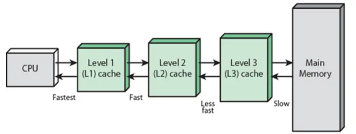
I’ve written previously about the “Memory Wall” stemming from a widening CPU <=> Main Memory performance gap. Among the steps taken by chip designers to mitigate the issue is the placement of smaller, faster pockets of SRAM nearer the CPU (illustrated below):

Level 3 (L3) represents the Last Level Cache (LLC) in the example above, and is the last (and slowest) stop within the cache hierarchy before the system must endure the long trek out to Main Memory. Among LLC design choices is the “inclusion policy” – i.e., whether or not the contents of the smaller caches shall be a subset of the LLC.

NOTE: For an in-depth discussion on CPU microarchitecture and squeezing the most performance from it, check out our book Performance Analysis and Tuning on Modern CPUs.1

Inclusion Policy

LLC inclusion policy falls into three camps: inclusive, exclusive, and non-inclusive. If all cache blocks of the smaller caches must also reside in the LLC, then that LLC is “inclusive”. If the LLC only contains blocks which are *not* present in the smaller caches, then that LLC is “exclusive”. And finally, if the LLC is neither strictly inclusive nor exclusive of the smaller caches, it is labeled “non-inclusive”.

Benefits of an inclusive LLC include greatly simplified cache coherency since less traffic must traverse all levels of the cache hierarchy to achieve its aim. Simply put, when the LLC contains all blocks from all levels of the cache hierarchy, it becomes the “one stop shop” for coherency info. However, one of the drawbacks is wasted capacity. As a matter of fact, a long held belief pinpointed squandered memory as the main drawback of an inclusive policy. But its true disadvantage is a more insidious side-effect – “backward invalidations”.

Inclusive LLC & Backward Invalidations

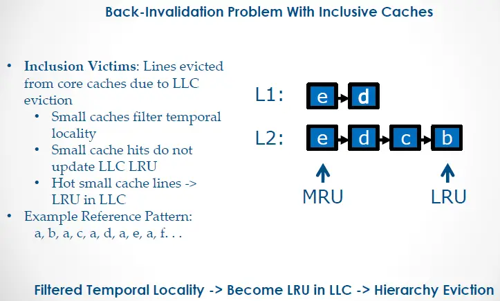
Recall that an inclusive policy dictates that all blocks of the smaller caches *must* also reside in the LLC. This means that any block evicted from the LLC must be evicted from the smaller caches to maintain compliance. This is referred to as a “backward invalidation”.

Imagine a hypothetical CPU as pictured above with the L2 designated as its inclusive LLC. Letters ‘a’ thru ‘e’ depict cache blocks in the cache hierarchy. If the CPU core references blocks in the pattern depicted (a -> b -> a -> c -> a -> d and so forth), the LLC will fill up with each of these blocks until the core requests block ‘e’. The LLC reaches max capacity at that point, and so must evict another block based on its LRU history table. The inclusion victim would be block ‘a’ despite the fact that this block remains at the MRU end of the L1’s history table. In compliance with inclusion policy, the L1 evicts block ‘a’, as well. Imagine the performance hit incurred from this repeated L1 eviction of hot cache block ‘a’!

Filtered temporal information between the L1 and LLC forms the crux of the issue. The LLC only knows about compulsory cache miss events across all levels, but not about cache hit updates for those blocks. Mitigating this issue, therefore, requires opening that channel of communication back to the LLC. Intel attempted at least two different solutions to this issue: Temporal Locality Hints (TLH) and Query Based Selection (QBS).

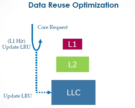
Temporal Locality Hints

TLH conveys temporal info about hot L1 cache blocks back to the LLC. This makes it far less likely for the LLC to choose those blocks for eviction. The drawback, however, is all that extra bandwidth required between the L1 and LLC. In fact, this feature was once configurable as a BIOS option on CPUs as recent as Westmere. It was called “Data Reuse Optimization”:

However, that BIOS option disappeared on subsequent CPU releases. Is this because Intel replaced TLH with something else? Or did they just remove it as a configuration option? I don’t know. Worse still, I have no Westmere system on which to perform a demo for you. Sorry, guys.

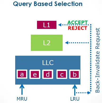
Query Based Selection

Each year, I’d get invited to the Intel HPC Roundtable where we’d discuss microarchitectural details of upcoming chip releases. These intimate workshops with Intel Fellows and Distinguished Engineers facilitated the kind of deep dives and Q&As that weren’t possible on public forums.

Here’s what I scribbled in my notes from one of the speakers on the subject of the upcoming Broadwell server CPU release at Intel HPC Roundtable 2015:

“posted interrupts, page modification logging, cache QoS enforcement, memory BW monitoring, HW-controlled power mgmt., improved page miss handling/page table walking, Query Based Selection (L3 won’t evict before querying core)“

And that’s exactly how QBS works – before selecting a block as an inclusion victim, it first queries the L1 for approval:

I flew back home to Chicago excited and eager to get my hands on the pre-release Broadwell evaluation CPU for testing.2 But my benchmark results left me scratching my head. Maybe QBS was not all it was touted to be. So, I reached out to Intel Engineering with my benchmark code and test results, only to hear back that they’d given up on QBS prior to release due to “unresolved issues.” Well, at least Intel came through with the “Cache QoS Enforcement” promise as a workaround.

Embracing Non-inclusive Last Level Caches

After Broadwell, Intel finally joined the AMD camp and adopted non-inclusive LLCs with the release of Skylake. This permitted them to reduce the LLC footprint while considerably boosting L2 size. But does it live up to billing? Let’s see!

Demo

Our demo includes two machines: one Haswell-based (inclusive LLC) and the other Cascade Lake-based (non-inclusive LLC). I’ll grab my favorite all-purpose benchmark tool, stress-ng, and use its ‘flip’ VM stressor as a stand-in for our “low latency application”. The LLC-hogging application will be played by the ‘read64’ VM stressor. We’ll conduct both tests on the 2nd socket of each machine (all odd-numbered cores) where all cores are isolated from the scheduler. We’ll use core 3 for ‘flip’ and core 7 for ‘read64’.

“That’s odd. Why would you skip core 1, the first core on the 2nd socket?” Oh, you know full well why I’m not using that core! Don’t play with me!

Haswell: Inclusive Last Level Cache

This Haswell system contains 32KB of L1d and 20MB of LLC as shown below:

[mdawson@haswell ~]$ lscpu
Architecture:          x86_64
CPU op-mode(s):        32-bit, 64-bit
Byte Order:            Little Endian
CPU(s):                16
On-line CPU(s) list:   0-15
Thread(s) per core:    1
Core(s) per socket:    8
Socket(s):             2
NUMA node(s):          2
Vendor ID:             GenuineIntel
CPU family:            6
Model:                 63
Model name:            Intel(R) Xeon(R) CPU E5-2667 v3 @ 3.20GHz
Stepping:              2
CPU MHz:               3199.738
BogoMIPS:              6403.88
Virtualization:        VT-x
L1d cache:             32K
L1i cache:             32K
L2 cache:              256K
L3 cache:              20480K
NUMA node0 CPU(s):     0,2,4,6,8,10,12,14
NUMA node1 CPU(s):     1,3,5,7,9,11,13,15

Let’s grab a baseline run of ‘flip’ on core 3 using a 32KB working set which neatly fits the L1d:

[mdawson@haswell ~]$ perf stat -r 5 -d numactl --membind=1 stress-ng --vm 1 --taskset 3 --vm-keep --vm-bytes 32k --vm-method flip --metrics-brief --timeout 15s
stress-ng: info:  [80547] dispatching hogs: 1 vm
stress-ng: info:  [80547] successful run completed in 15.00s
stress-ng: info:  [80547] stressor       bogo ops real time  usr time  sys time   bogo ops/s   bogo ops/s
stress-ng: info:  [80547]                           (secs)    (secs)    (secs)   (real time) (usr+sys time)
stress-ng: info:  [80547] vm              1052649     15.00     14.87      0.12     70175.86     70223.42
stress-ng: info:  [80568] dispatching hogs: 1 vm
stress-ng: info:  [80568] successful run completed in 15.00s
stress-ng: info:  [80568] stressor       bogo ops real time  usr time  sys time   bogo ops/s   bogo ops/s
stress-ng: info:  [80568]                           (secs)    (secs)    (secs)   (real time) (usr+sys time)
stress-ng: info:  [80568] vm              1051884     15.00     14.87      0.12     70124.85     70172.38
stress-ng: info:  [80584] dispatching hogs: 1 vm
stress-ng: info:  [80584] successful run completed in 15.00s
stress-ng: info:  [80584] stressor       bogo ops real time  usr time  sys time   bogo ops/s   bogo ops/s
stress-ng: info:  [80584]                           (secs)    (secs)    (secs)   (real time) (usr+sys time)
stress-ng: info:  [80584] vm              1052379     15.00     14.87      0.12     70157.86     70205.40
stress-ng: info:  [80601] dispatching hogs: 1 vm
stress-ng: info:  [80601] successful run completed in 15.00s
stress-ng: info:  [80601] stressor       bogo ops real time  usr time  sys time   bogo ops/s   bogo ops/s
stress-ng: info:  [80601]                           (secs)    (secs)    (secs)   (real time) (usr+sys time)
stress-ng: info:  [80601] vm              1052289     15.00     14.87      0.12     70151.86     70199.40
stress-ng: info:  [80618] dispatching hogs: 1 vm
stress-ng: info:  [80618] successful run completed in 15.00s
stress-ng: info:  [80618] stressor       bogo ops real time  usr time  sys time   bogo ops/s   bogo ops/s
stress-ng: info:  [80618]                           (secs)    (secs)    (secs)   (real time) (usr+sys time)
stress-ng: info:  [80618] vm              1052280     15.00     14.87      0.12     70151.25     70198.80

 Performance counter stats for 'numactl --membind=1 stress-ng --vm 1 --taskset 3 --vm-keep --vm-bytes 32k --vm-method flip --metrics-brief --timeout 15s' (5 runs):

         15,005.64 msec task-clock                #    1.000 CPUs utilized            ( +-  0.00% )
                14      context-switches          #    0.001 K/sec                    ( +-  2.71% )
                 0      cpu-migrations            #    0.000 K/sec
             1,704      page-faults               #    0.114 K/sec
    50,584,401,411      cycles                    #    3.371 GHz                      ( +-  0.01% )  (49.99%)
   181,359,934,141      instructions              #    3.59  insn per cycle           ( +-  0.01% )  (62.49%)
    17,583,120,821      branches                  # 1171.768 M/sec                    ( +-  0.01% )  (74.99%)
         2,244,595      branch-misses             #    0.01% of all branches          ( +-  0.76% )  (87.50%)
    44,492,963,211      L1-dcache-loads           # 2965.083 M/sec                    ( +-  0.01% )  (37.52%)
        61,653,565      L1-dcache-load-misses     #    0.14% of all L1-dcache hits    ( +-  0.85% )  (37.51%)
           254,253      LLC-loads                 #    0.017 M/sec                    ( +-  1.34% )  (37.50%)
           146,656      LLC-load-misses           #   57.68% of all LL-cache hits     ( +-  1.51% )  (37.48%)

         15.007112 +- 0.000626 seconds time elapsed  ( +-  0.00% )

Bogo ops/s measures consistently at slightly over 70,000 per run. It maintains a 3.59 IPC, L1d throughput of 2.96GB/s, and LLC throughput of 17KB/s.

Now, let’s re-run ‘flip’ with ‘read64’ concurrently executing on core 7 with a 21MB working set size:3

[mdawson@haswell ~]$ perf stat -r 5 -d numactl --membind=1 stress-ng --vm 1 --taskset 3 --vm-keep --vm-bytes 32k --vm-method flip --metrics-brief --timeout 15s
stress-ng: info:  [80393] dispatching hogs: 1 vm
stress-ng: info:  [80393] successful run completed in 15.00s
stress-ng: info:  [80393] stressor       bogo ops real time  usr time  sys time   bogo ops/s   bogo ops/s
stress-ng: info:  [80393]                           (secs)    (secs)    (secs)   (real time) (usr+sys time)
stress-ng: info:  [80393] vm              1028772     15.00     14.79      0.20     68583.61     68630.55
stress-ng: info:  [80416] dispatching hogs: 1 vm
stress-ng: info:  [80416] successful run completed in 15.00s
stress-ng: info:  [80416] stressor       bogo ops real time  usr time  sys time   bogo ops/s   bogo ops/s
stress-ng: info:  [80416]                           (secs)    (secs)    (secs)   (real time) (usr+sys time)
stress-ng: info:  [80416] vm              1028232     15.00     14.77      0.22     68547.73     68594.53
stress-ng: info:  [80441] dispatching hogs: 1 vm
stress-ng: info:  [80441] successful run completed in 15.00s
stress-ng: info:  [80441] stressor       bogo ops real time  usr time  sys time   bogo ops/s   bogo ops/s
stress-ng: info:  [80441]                           (secs)    (secs)    (secs)   (real time) (usr+sys time)
stress-ng: info:  [80441] vm              1026774     15.00     14.78      0.21     68450.44     68497.26
stress-ng: info:  [80462] dispatching hogs: 1 vm
stress-ng: info:  [80462] successful run completed in 15.00s
stress-ng: info:  [80462] stressor       bogo ops real time  usr time  sys time   bogo ops/s   bogo ops/s
stress-ng: info:  [80462]                           (secs)    (secs)    (secs)   (real time) (usr+sys time)
stress-ng: info:  [80462] vm              1018467     15.00     14.75      0.24     67896.67     67943.10
stress-ng: info:  [80484] dispatching hogs: 1 vm
stress-ng: info:  [80484] successful run completed in 15.00s
stress-ng: info:  [80484] stressor       bogo ops real time  usr time  sys time   bogo ops/s   bogo ops/s
stress-ng: info:  [80484]                           (secs)    (secs)    (secs)   (real time) (usr+sys time)
stress-ng: info:  [80484] vm              1020240     15.00     14.76      0.23     68014.82     68061.37

 Performance counter stats for 'numactl --membind=1 stress-ng --vm 1 --taskset 3 --vm-keep --vm-bytes 32k --vm-method flip --metrics-brief --timeout 15s' (5 runs):

         15,006.57 msec task-clock                #    1.000 CPUs utilized            ( +-  0.00% )
                15      context-switches          #    0.001 K/sec                    ( +-  2.60% )
                 0      cpu-migrations            #    0.000 K/sec
             1,704      page-faults               #    0.114 K/sec
    50,357,946,125      cycles                    #    3.356 GHz                      ( +-  0.04% )  (49.98%)
   176,607,210,201      instructions              #    3.51  insn per cycle           ( +-  0.20% )  (62.48%)
    17,122,614,281      branches                  # 1141.008 M/sec                    ( +-  0.20% )  (74.99%)
         2,241,031      branch-misses             #    0.01% of all branches          ( +-  0.96% )  (87.49%)
    43,313,418,811      L1-dcache-loads           # 2886.296 M/sec                    ( +-  0.22% )  (37.52%)
        59,635,656      L1-dcache-load-misses     #    0.14% of all L1-dcache hits    ( +-  0.80% )  (37.52%)
         1,894,194      LLC-loads                 #    0.126 M/sec                    ( +-  7.24% )  (37.50%)
         1,750,423      LLC-load-misses           #   92.41% of all LL-cache hits     ( +-  7.08% )  (37.48%)

         15.007929 +- 0.000884 seconds time elapsed  ( +-  0.01% )

With core 7 polluting the shared LLC, ‘flip’ drops from ~70,000 to ~68,000 bogo ops/s. Notice the drop in IPC from 3.59 to 3.51, L1d throughput drop from 2.96GB/s to 2.89GB/s, and LLC throughput increase from 17KB/s to 126KB/s. Despite a small, L1d-sized working set (32KB), messiness at the LLC level still adversely impacts core 3’s private core cache.

How does a non-inclusive LLC change matters, if at all?

Cascade Lake: Non-inclusive Last Level Cache

This Cascade Lake system contains 32KB of L1d cache and 25MB of LLC as depicted below:

[mdawson@cascadelake ~]$ lscpu
Architecture:        x86_64
CPU op-mode(s):      32-bit, 64-bit
Byte Order:          Little Endian
CPU(s):              16
On-line CPU(s) list: 0-15
Thread(s) per core:  1
Core(s) per socket:  8
Socket(s):           2
NUMA node(s):        2
Vendor ID:           GenuineIntel
CPU family:          6
Model:               85
Model name:          Intel(R) Xeon(R) Gold 6244 CPU @ 3.60GHz
Stepping:            7
CPU MHz:             4299.863
BogoMIPS:            7200.00
L1d cache:           32K
L1i cache:           32K
L2 cache:            1024K
L3 cache:            25344K
NUMA node0 CPU(s):   0,2,4,6,8,10,12,14
NUMA node1 CPU(s):   1,3,5,7,9,11,13,15

Just like in our previous Haswell demo, we’ll grab a baseline run of ‘flip’ on core 3 with a 32KB working set which fits our L1d cache:

[mdawson@cascadelake ~]$ perf stat -r 5 -d numactl --membind=1 stress-ng --vm 1 --taskset 3 --vm-keep --vm-bytes 32k --vm-method flip --metrics-brief --timeout 15s
stress-ng: info:  [389059] setting to a 15 second run per stressor
stress-ng: info:  [389059] dispatching hogs: 1 vm
stress-ng: info:  [389059] stressor       bogo ops real time  usr time  sys time   bogo ops/s     bogo ops/s
stress-ng: info:  [389059]                           (secs)    (secs)    (secs)   (real time) (usr+sys time)
stress-ng: info:  [389059] vm              1361427     15.00     14.62      0.31     90760.78       91187.34
stress-ng: info:  [389059] successful run completed in 15.00s
stress-ng: info:  [389064] setting to a 15 second run per stressor
stress-ng: info:  [389064] dispatching hogs: 1 vm
stress-ng: info:  [389064] stressor       bogo ops real time  usr time  sys time   bogo ops/s     bogo ops/s
stress-ng: info:  [389064]                           (secs)    (secs)    (secs)   (real time) (usr+sys time)
stress-ng: info:  [389064] vm              1361232     15.00     14.62      0.31     90747.84       91174.28
stress-ng: info:  [389064] successful run completed in 15.00s
stress-ng: info:  [389069] setting to a 15 second run per stressor
stress-ng: info:  [389069] dispatching hogs: 1 vm
stress-ng: info:  [389069] stressor       bogo ops real time  usr time  sys time   bogo ops/s     bogo ops/s
stress-ng: info:  [389069]                           (secs)    (secs)    (secs)   (real time) (usr+sys time)
stress-ng: info:  [389069] vm              1385590     15.00     14.61      0.32     92371.71       92805.76
stress-ng: info:  [389069] successful run completed in 15.00s
stress-ng: info:  [389077] setting to a 15 second run per stressor
stress-ng: info:  [389077] dispatching hogs: 1 vm
stress-ng: info:  [389077] stressor       bogo ops real time  usr time  sys time   bogo ops/s     bogo ops/s
stress-ng: info:  [389077]                           (secs)    (secs)    (secs)   (real time) (usr+sys time)
stress-ng: info:  [389077] vm              1361349     15.00     14.62      0.31     90755.72       91182.12
stress-ng: info:  [389077] successful run completed in 15.00s
stress-ng: info:  [389081] setting to a 15 second run per stressor
stress-ng: info:  [389081] dispatching hogs: 1 vm
stress-ng: info:  [389081] stressor       bogo ops real time  usr time  sys time   bogo ops/s     bogo ops/s
stress-ng: info:  [389081]                           (secs)    (secs)    (secs)   (real time) (usr+sys time)
stress-ng: info:  [389081] vm              1361366     15.00     14.62      0.31     90756.78       91183.26
stress-ng: info:  [389081] successful run completed in 15.00s

 Performance counter stats for 'numactl --membind=1 stress-ng --vm 1 --taskset 3 --vm-keep --vm-bytes 32k --vm-method flip --metrics-brief --timeout 15s' (5 runs):

         15,003.53 msec task-clock:u              #    1.000 CPUs utilized            ( +-  0.00% )
                 0      context-switches:u        #    0.000 /sec
                 0      cpu-migrations:u          #    0.000 /sec
               917      page-faults:u             #   61.118 /sec
    62,471,828,843      cycles:u                  #    4.164 GHz                      ( +-  0.01% )  (87.50%)
   252,455,743,745      instructions:u            #    4.04  insn per cycle           ( +-  0.15% )  (87.50%)
    28,372,743,612      branches:u                #    1.891 G/sec                    ( +-  0.08% )  (87.50%)
         2,840,043      branch-misses:u           #    0.01% of all branches          ( +-  1.82% )  (87.50%)
    62,138,602,359      L1-dcache-loads:u         #    4.142 G/sec                    ( +-  0.23% )  (87.50%)
       165,323,553      L1-dcache-load-misses:u   #    0.27% of all L1-dcache accesses  ( +-  1.64% )  (87.50%)
            22,070      LLC-loads:u               #    1.471 K/sec                    ( +-  0.18% )  (87.50%)
            15,785      LLC-load-misses:u         #   71.86% of all LL-cache accesses  ( +-  0.13% )  (87.50%)

         15.004840 +- 0.000385 seconds time elapsed  ( +-  0.00% )

In this case, bogo ops/s clocks in around 91,000 per run. It maintains a 4.04 IPC, L1d throughput of 4.14GB/s, and LLC throughput of ~1.5KB/s.

Now, let’s re-run ‘flip’ with ‘read64’ concurrently executing on core 7 with a 26MB working set size:4

[mdawson@cascadelake ~]$ perf stat -r 5 -d numactl --membind=1 stress-ng --vm 1 --taskset 3 --vm-keep --vm-bytes 32k --vm-method flip --metrics-brief --timeout 15s
stress-ng: info:  [388919] setting to a 15 second run per stressor
stress-ng: info:  [388919] dispatching hogs: 1 vm
stress-ng: info:  [388919] stressor       bogo ops real time  usr time  sys time   bogo ops/s     bogo ops/s
stress-ng: info:  [388919]                           (secs)    (secs)    (secs)   (real time) (usr+sys time)
stress-ng: info:  [388919] vm              1360767     15.00     14.61      0.32     90716.70       91143.13
stress-ng: info:  [388919] successful run completed in 15.00s
stress-ng: info:  [388928] setting to a 15 second run per stressor
stress-ng: info:  [388928] dispatching hogs: 1 vm
stress-ng: info:  [388928] stressor       bogo ops real time  usr time  sys time   bogo ops/s     bogo ops/s
stress-ng: info:  [388928]                           (secs)    (secs)    (secs)   (real time) (usr+sys time)
stress-ng: info:  [388928] vm              1385074     15.00     14.61      0.32     92337.25       92771.20
stress-ng: info:  [388928] successful run completed in 15.00s
stress-ng: info:  [388936] setting to a 15 second run per stressor
stress-ng: info:  [388936] dispatching hogs: 1 vm
stress-ng: info:  [388936] stressor       bogo ops real time  usr time  sys time   bogo ops/s     bogo ops/s
stress-ng: info:  [388936]                           (secs)    (secs)    (secs)   (real time) (usr+sys time)
stress-ng: info:  [388936] vm              1385027     15.00     14.60      0.32     92334.09       92830.23
stress-ng: info:  [388936] successful run completed in 15.00s
stress-ng: info:  [388944] setting to a 15 second run per stressor
stress-ng: info:  [388944] dispatching hogs: 1 vm
stress-ng: info:  [388944] stressor       bogo ops real time  usr time  sys time   bogo ops/s     bogo ops/s
stress-ng: info:  [388944]                           (secs)    (secs)    (secs)   (real time) (usr+sys time)
stress-ng: info:  [388944] vm              1361188     15.00     14.62      0.31     90744.86       91171.33
stress-ng: info:  [388944] successful run completed in 15.00s
stress-ng: info:  [388952] setting to a 15 second run per stressor
stress-ng: info:  [388952] dispatching hogs: 1 vm
stress-ng: info:  [388952] stressor       bogo ops real time  usr time  sys time   bogo ops/s     bogo ops/s
stress-ng: info:  [388952]                           (secs)    (secs)    (secs)   (real time) (usr+sys time)
stress-ng: info:  [388952] vm              1361205     15.00     14.61      0.32     90746.03       91172.47
stress-ng: info:  [388952] successful run completed in 15.00s

 Performance counter stats for 'numactl --membind=1 stress-ng --vm 1 --taskset 3 --vm-keep --vm-bytes 32k --vm-method flip --metrics-brief --timeout 15s' (5 runs):

         15,003.56 msec task-clock:u              #    1.000 CPUs utilized            ( +-  0.00% )
                 0      context-switches:u        #    0.000 /sec
                 0      cpu-migrations:u          #    0.000 /sec
               917      page-faults:u             #   61.118 /sec
    62,457,928,284      cycles:u                  #    4.163 GHz                      ( +-  0.02% )  (87.49%)
   252,469,328,307      instructions:u            #    4.04  insn per cycle           ( +-  0.17% )  (87.50%)
    28,369,514,296      branches:u                #    1.891 G/sec                    ( +-  0.09% )  (87.50%)
         2,889,046      branch-misses:u           #    0.01% of all branches          ( +-  0.69% )  (87.50%)
    62,125,500,337      L1-dcache-loads:u         #    4.141 G/sec                    ( +-  0.27% )  (87.50%)
       162,790,289      L1-dcache-load-misses:u   #    0.26% of all L1-dcache accesses  ( +-  2.14% )  (87.50%)
            22,027      LLC-loads:u               #    1.468 K/sec                    ( +-  0.13% )  (87.50%)
            15,768      LLC-load-misses:u         #   71.65% of all LL-cache accesses  ( +-  0.58% )  (87.50%)

        15.0046476 +- 0.0000781 seconds time elapsed  ( +-  0.00% )

Even though core 7 swamps the LLC with reads, the ‘flip’ workload throughput never drops, and IPC & L1d/LLC throughput rates remain the same between setups! Cascade Lake’s non-inclusive policy protected the performance of our low-latency application!

Be Inclusive Everywhere Except the LLC

We should strive for inclusivity in our personal and professional lives, and in society as a whole for the betterment of humanity. But when it comes to your CPU Last Level Cache, you might want to reconsider. And don’t forget to check your chosen cloud instance types. If they’re supported by anything earlier than Skylake, then you may just be suffering from a form of noisy neighbor you never anticipated.

1    Paid affiliate link2    Lots of HFT firms are on Early Release Programs with chip manufacturers to test CPUs prior to GA release.3    perf stat -r 5 -d numactl –membind=1 stress-ng –vm 1 –taskset 7 –vm-keep –vm-bytes 21m –vm-method read64 –metrics-brief –timeout 15s4    perf stat -r 5 -d numactl –membind=1 stress-ng –vm 1 –taskset 7 –vm-keep –vm-bytes 26m –vm-method read64 –metrics-brief –timeout 15s

The post Last Level Cache: Where It’s Bad To Be Inclusive appeared first on JabPerf Corp.

Estimated reading time: 11 minutes

“Who hurt you?“

That’s the recurring question every confirmed bachelor, Lothario, and playboy expects to hear around this Valentine’s Day Season. That time of year when couples exchange gifts of love, share romantic dinners, or whisk away on a mini-trip. Meanwhile, free-wheeling casual daters skillfully avoid the festivities with their multiple paramours with well-rehearsed scripts criticizing the holiday’s emptiness and commercial nature. Once that Celebration of Exclusivity passes, they come back out of hiding, ready to mingle! But why is that? Could it just be that some of us enjoy the excitement of sparking a romance with new and interesting people? Or might it stem from a fear of commitment due to some past heartbreak? “Who hurt you?” assumes the latter.

You and I have formed a pretty solid bond over these past couple years, so I’ll come clean with you: I fear commitment. . . to the 1st CPU core. And not just core 0, either, which we all know usually catches the brunt of interrupts and typically is singled-out as a house-keeping core. I’m talkin’ about the 1st core on *any* CPU socket. And you’re right – it’s not due to some free-wheeling excitement gained from the willy-nilly scheduling of threads across cores. It’s because the 1st CPU core once hurt me deeply, and I haven’t looked at it the same way since. Here’s my story.

Table of contents

• The 1st CPU Core and How We Met
• Cracks Begin To Show
• The 1st CPU Core and its Wandering Eye
  • How rq_affinity *Used* to Work
• The 1st CPU Core Attempts To Rekindle Our Flame
  • Testing the Updated rq_affinity = 1
  • Testing the Updated rq_affinity = 2
• What We Had Was Beautiful But. . .

The 1st CPU Core and How We Met

My meet-cute with the 1st CPU core began around 2014. RHEL 7 had just been released with very few in the HFT space considering a migration from RHEL 6.8 and its 2.6.32 kernel until they could suss out all latency gotchas in RHEL 7’s 3.10.0 kernel. It was under this backdrop that I worked with a startup Options Trading Group of a Chicago-based HFT firm.

I deployed the usual configurations you’d expect for low latency, many of which I’ve alluded to in past articles. Most important was core isolation (isolcpus) on the 2nd CPU (odd-numbered cores), home to the NIC’s PCIe lanes. Free from the vagaries of the Linux kernel scheduler, these cores served as low-jitter locations for latency-critical application threads. One of the more important threads we pinned to core 1, the 1st core on that 2nd socket. And for a few weeks, it was a fairy-tale affair. High IPC, low jitter, low latency – the pairing seemed destined! But nothing lasts forever, does it?

Cracks Begin To Show

“Mark, we’re suddenly experiencing sporadic latency spikes of over 1ms on core 1!”

Weeks had gone by without a hitch on the Options Trading Group’s system. So how could this be? Now, for those of you who have never serviced customers in IT, I’ll let you in on a little secret – they *never* tell you the whole story. It’s always “No, we didn’t change anything. We were just moseying along and then BOOM!” But hey, it is what it is. So, I fired up the FTrace facility and began tracking scheduler events on that core:

[root@eltoro]# echo sched_switch > /sys/kernel/debug/tracing/current_tracer
[root@eltoro]# echo latency-format > /sys/kernel/debug/tracing/trace_options

Here’s some of the tracing output I found after enabling those FTrace options:

TradeApp-31594   1d.s.. 70251098us!:  31594:115:R   + [001]     6:120:R ksoftirqd
TradeApp-31594   1d.... 70252191us!:  31594:115:R ==> [001]     6:120:R ksoftirqd
ksoftirqd-6      1d.... 70252599us!:      6:120:S ==> [001] 31594:115:R TradeApp

<<< above represents ~400 microsecond scheduling latency >>>

TradeApp-31594   1d.s.. 85246192us!:  31594:115:R   + [001]     6:120:R ksoftirqd
TradeApp-31594   1d.... 85246652us!:  31594:115:R ==> [001]     6:120:R ksoftirqd
ksoftirqd-6      1d.... 85262686us!:      6:120:R ==> [001] 31594:115:R TradeApp

<<< above represents a whopping 16 millisecond scheduling latency >>>

Ksoftirqd was taking as much as 16 *milliseconds* of cpu time from the trading application thread! This kernel thread jumps into action in process-context when the interrupt-context softirq is overwhelmed with work and, therefore, needs to offload it to a schedule-able entity. But what type of work overloaded the softirq so much that it had to enlist the help of ksoftirqd?

For this, I enabled the function_graph tracer in FTrace to track the flow of kernel functions called during ksoftirqd‘s runtime. What did I find? A bunch of block request queue completion work (i.e., the cleaning of block layer structures created during the process of handling I/O) from the megasas disk I/O controller.

But why? No one pinned the megasas driver IRQ to core 1. So why was all its associated background processing running there?

The 1st CPU Core and its Wandering Eye

Every now and then, you might miss a configuration step or two, even while using configuration management tools like Puppet or Ansible. So I verified my IRQ-assignment assumptions by checking /proc/interrupts, which confirmed my understanding. However, I *did* find a torrent of “Function Call Interrupts” (or CAL in /proc/interrupts parlance) hitting our beloved core 1:

           CPU0       CPU1       CPU2       CPU3       CPU4       CPU5       CPU6       CPU7       
  0:         47          0          0          0          0          0          0          0   IO-APIC-edge      timer
  1:         25          0          0          0          0          0          0          0   IO-APIC-edge      i8042
  8:          1          0          0          0          0          0          0          0   IO-APIC-edge      rtc0
  9:        528          0          0        287          0          0          0          0   IO-APIC-fasteoi   acpi
 12:        207          0          0          0          0          0          0          0   IO-APIC-edge      i8042
 16:        493          0        187          0          0          0          0          0   IO-APIC-fasteoi   ehci_hcd:usb1, nouveau
 17:      29465          0          0          0          0          0          0          0   IO-APIC-fasteoi   ath9k, snd_hda_intel
 19:          0          0          0          0          0          0          0          0   IO-APIC-fasteoi   xhci_hcd:usb3
 23:       9352          0          0          0          0          0          0          0   IO-APIC-fasteoi   ehci_hcd:usb2
 45:          0          0          0          0          0          0          0          0   PCI-MSI-edge      eth0
 46:     192342          0          0          0          0          0          0          0   PCI-MSI-edge      ahci
 47:         14          0          0          0          0          0          0          0   PCI-MSI-edge      mei
 48:        294          0          0          0          0          0          0          0   PCI-MSI-edge      snd_hda_intel
NMI:          0          0          0          0          0          0          0          0   Non-maskable interrupts
LOC:     552219    1010298    2272333    3179890    1445484    1226202    1800191    1894825   Local timer interrupts
SPU:          0          0          0          0          0          0          0          0   Spurious interrupts
PMI:          0          0          0          0          0          0          0          0   Performance monitoring interrupts
IWI:          0          0          0          0          0          0          0          0   IRQ work interrupts
RTR:          7          0          0          0          0          0          0          0   APIC ICR read retries
RES:      18708       9550        771        528        129        170        151        139   Rescheduling interrupts
CAL:        711    9153934       1312       1261       1446       1411       1433       1432   Function call interrupts
TLB:       4493       6108       4981       5014       1788       2327       1967        914   TLB shootdowns
TRM:          0          0          0          0          0          0          0          0   Thermal event interrupts

That’s 3 orders of magnitude more CALs on core 1 than any other core! Further debugging and source code reading (explained in the next section) revealed the culprit as the /sys/block/sda/queue/rq_affinity setting. From the kernel docs:

“If this option is ‘1’, the block layer will migrate request completions to the
cpu “group” that originally submitted the request. For some workloads this
provides a significant reduction in CPU cycles due to caching effects.”

And of course, it was at this point that I noticed another core on that same CPU socket performing a heavy stream of writes to the disk attached to the megasas driver. “Oh yeah, Mark, we pinned a new thread to core 3 on that socket to perform our data writes. Did we forget to mention that?” *sigh*

Just to make sure you all are following me, here’s a recap: Core 1 and I agreed that it would dedicate itself to our trading workload, but then weeks later some other I/O workload came struttin’ by and stole its attention away from me. Really? Just like that, huh? What ever happened to trust? To fidelity? To ’til decommission do us part’?!

This I/O-heavy workload on core 3 adversely impacted latency on core 1 due to rq_affinity interrupting it via CALs to perform block request completion cleanup (as we’ll learn in the next section). But why was it always core 1? Why not share it with other cores within that same LLC-sharing “group”? To answer that, we gotta read the source.

How rq_affinity *Used* to Work

The workhorse for rq_affinity is the __blk_complete_request() function shown below from a 2.6.32 kernel release:

void __blk_complete_request(struct request *req)
{
	struct request_queue *q = req->q;
	unsigned long flags;
	int ccpu, cpu, group_cpu;

	BUG_ON(!q->softirq_done_fn);

	local_irq_save(flags);
	cpu = smp_processor_id();
	group_cpu = blk_cpu_to_group(cpu);

	/*
	 * Select completion CPU
	 */
	if (test_bit(QUEUE_FLAG_SAME_COMP, &q->queue_flags) && req->cpu != -1)
		ccpu = req->cpu;
	else
		ccpu = cpu;

	if (ccpu == cpu || ccpu == group_cpu) {
		struct list_head *list;
do_local:
		list = &__get_cpu_var(blk_cpu_done);
		list_add_tail(&req->csd.list, list);

		/*
		 * if the list only contains our just added request,
		 * signal a raise of the softirq. If there are already
		 * entries there, someone already raised the irq but it
		 * hasn't run yet.
		 */
		if (list->next == &req->csd.list)
			raise_softirq_irqoff(BLOCK_SOFTIRQ);
	} else if (raise_blk_irq(ccpu, req))
		goto do_local;

	local_irq_restore(flags);

Here, it finds the core that is currently servicing the IRQ (cpu variable), compares it to the core identified in the block I/O request struct as the originator of the I/O (req->cpu variable), and checks if rq_affinity is set (i.e., QUEUE_FLAG_SAME_COMP flag). If set, and both cores are not one and the same OR do not belong to the same LLC-sharing group, it will interrupt the originating core to process the block request completion using the raise_blk_irq() function:

/*
 * Setup and invoke a run of 'trigger_softirq' on the given cpu.
 */
static int raise_blk_irq(int cpu, struct request *rq)
{
	if (cpu_online(cpu)) {
		struct call_single_data *data = &rq->csd;

		data->func = trigger_softirq;
		data->info = rq;
		data->flags = 0;

		__smp_call_function_single(cpu, data, 0);
		return 0;
	}

	return 1;
}

Aha, so now we know the source of all those CALs we saw in /proc/interrupts – the __smp_call_function_single() function!

Finally, how is that req->cpu variable set up in the first place? Well, let’s take a look at a snippet of the function that starts it all, __make_request():

static int __make_request(struct request_queue *q, struct bio *bio)
{
	struct request *req;
	int el_ret;
	unsigned int bytes = bio->bi_size;
	const unsigned short prio = bio_prio(bio);
	const int sync = bio_sync(bio);
	const int unplug = bio_unplug(bio);
	int rw_flags;spin_lock_irq(q->queue_lock);
	. . .
	. . .
	. . .
	if (test_bit(QUEUE_FLAG_SAME_COMP, &q->queue_flags) ||
	    bio_flagged(bio, BIO_CPU_AFFINE))
		req->cpu = blk_cpu_to_group(smp_processor_id());
  . . .
  . . .
  . . .

Ok, so this all seems reasonable now, right? We had cores 1 and 3 in the same “group”, with rq_affinity enabled, and the megasas IRQ pinned to a core which was NOT part of that group. Case closed, right? Wrong! We still don’t know why core 1 is *always* the victim among all the cores on that second CPU socket.

Let’s take a look at the blk_cpu_to_group() function referenced in the code snippets above for more insight:

static inline int blk_cpu_to_group(int cpu)
{
#ifdef CONFIG_SCHED_MC
	const struct cpumask *mask = cpu_coregroup_mask(cpu);
	return cpumask_first(mask);
#elif defined(CONFIG_SCHED_SMT)
	return cpumask_first(topology_thread_cpumask(cpu));
#else
	return cpu;
#endif
}

Uh, what’s with that “_first” suffix to the cpumask_first() function? Makes me nervous. Hmm, maybe I’m being paranoid. Let’s check out its definition:

/**
 * cpumask_first - get the first cpu in a cpumask
 * @srcp: the cpumask pointer
 *
 * Returns >= nr_cpu_ids if no cpus set.
 */
static inline unsigned int cpumask_first(const struct cpumask *srcp)
{
	return find_first_bit(cpumask_bits(srcp), nr_cpumask_bits);
}

NOOOO!!! It *always* picks the first core in the group, thus causing core 1’s milliseconds-long hiccups! You broke my heart, core 1. You broke my heart. I’ll never trust the 1st core on any CPU socket with a low-latency assignment ever again, especially not when there’s a cpumask_first() function defined in the kernel just waiting for someone to use in the future!

The 1st CPU Core Attempts To Rekindle Our Flame

Nowadays, rq_affinity offers an extra option which makes the core that is generating all the I/O clean up after itself:

“For storage configurations that need to maximize distribution of completion
processing setting this option to ‘2’ forces the completion to run on the
requesting cpu (bypassing the “group” aggregation logic).“

It also removes any consideration about the “first core in the group” as depicted in this snippet from the same __blk_complete_request() function from a more recent kernel release:

/*
	 * Select completion CPU
	 */
	if (test_bit(QUEUE_FLAG_SAME_COMP, &q->queue_flags) && ccpu != -1) {
		if (!test_bit(QUEUE_FLAG_SAME_FORCE, &q->queue_flags))
			shared = cpus_share_cache(cpu, ccpu);
	} else
		ccpu = cpu;

	/*
	 * If current CPU and requested CPU share a cache, run the softirq on
	 * the current CPU. One might concern this is just like
	 * QUEUE_FLAG_SAME_FORCE, but actually not. blk_complete_request() is
	 * running in interrupt handler, and currently I/O controller doesn't
	 * support multiple interrupts, so current CPU is unique actually. This
	 * avoids IPI sending from current CPU to the first CPU of a group.
	 */
	if (ccpu == cpu || shared) {
		struct list_head *list;

But how can I be sure? When you go through a betrayal of this magnitude, you’re not eager to jump right back into that relationship. Let’s set up a test for this new setting on Rocky 8.6 (kernel release 4.18.0-372.9.1) using the fio microbenchmark and the osnoise latency tracker.

Testing the Updated rq_affinity = 1

For this test, we have isolated the cores of the 2nd CPU socket (all odd-numbered cores). The target disk IRQ is assigned to core 7, our fio microbenchmark is pinned to core 3, and rq_affinity is set to ‘1’ (the default).

In a separate window, I’ve set up the osnoise tracer to track any disturbance lasting for longer than a millisecond against any core on the 2nd CPU socket *except* core 3, where our fio workload will run:

[root@eltoro ~]# cd /sys/kernel/tracing/
[root@eltoro tracing]# echo osnoise > current_tracer
[root@eltoro tracing]# echo osnoise > set_event
[root@eltoro tracing]# echo "1,5,7,9,11,13,15" > osnoise/cpus
[root@eltoro tracing]# echo 1000 > osnoise/stop_tracing_us

In a separate window, I fire up fio to perform random writes for 300 seconds against a 5GB file using one thread pinned to core 3:

[root@eltoro ~]# fio -name=blogpost -numjobs=1 -cpus_allowed=3 -filename=/corefiles/mytest.file -direct=0 -rw=randwrite -bs=4k -size=5G -iodepth=64 -ioengine=libaio -time_based=1 -runtime=300

Once I hit ‘ENTER’ on the fio command, I start the trace in the other window like so:

[root@eltoro tracing]# echo 1 > tracing_on
[root@eltoro tracing]# cat trace_pipe

After a few seconds, the trace automatically stops and displays this output as its final few lines:

       . . .
       . . .
       . . .
       osnoise/7-13353 [007] d.h. 37384.833988: irq_noise: ahci[0000:87:00.0]:47 start 37384.833985696 duration 2390 ns
       osnoise/7-13353 [007] ..s. 37384.840123: softirq_noise:    BLOCK:4 start 37384.833988294 duration 6134479 ns
       osnoise/7-13353 [007] .... 37384.840124: sample_threshold: start 37384.833985490 duration 6138539 ns interference 2
[root@eltoro tracing]#

I keep reenabling the trace during the fio microbenchmark but the trace keeps stopping at lines showing disturbances only for core 7 from softirqs executing block-related code. This is great because it means that it’s not bugging core 1 like in older kernel releases! We get further proof from the preponderance of reported “BLOCK” softirqs, 256,724 in all (0 on the other cores), going to core 7 in /proc/softirqs:

[root@eltoro ~]# cat /proc/softirqs
                    CPU0       CPU1       CPU2       CPU3       CPU4       CPU5       CPU6       CPU7       CPU8       CPU9       CPU10      CPU11      CPU12      CPU13      CPU14      CPU15
          HI:          1          0          0          0          0          0          0          0          0          0          0          0          0          0          0          0
       TIMER:    1311064       4732       4732       4733       4732       4731       4731       4732       4731       4731       4731       4731       4731       4731       4731       4731
      NET_TX:      14369          1          2          1          2          0          1          0          1          0          0          0          2          0          1          0
      NET_RX:     547910        525     151351       2080          3          0          3          0          3          2          4          1          4          1          3          0
       BLOCK:        106          0          0          0          0          0          0     256724          0          0          0          0          0          0          0          0
    IRQ_POLL:          0          0          0          0          0          0          0          0          0          0          0          0          0          0          0          0
     TASKLET:      33514          0          0          0          0          0          0          0         19          0         64          0          0          0          0          0
       SCHED:          0          0          0          0          0          0          0          0          0          0          0          0          0          0          0          0
     HRTIMER:          0          0          0          0          0          0          0          0          0          0          0          0          0          0          0          0
         RCU:     999445       4754       4733       5599       4734       4765       4732       5147       4732       4823       4732       4767       4732       4816       4732       4751

Now let’s see what happens after a clean reboot with rq_affinity set to ‘2’.

Testing the Updated rq_affinity = 2

Everything is configured the exact same way as in the previous section except rq_affinity is now set to ‘2’. I fire up fio, then I commence tracing and begin reading from the pipe:

[root@eltoro tracing]# echo 1 > tracing_on
[root@eltoro tracing]# cat trace_pipe
       osnoise/5-2065  [005] d.h.   475.145177: irq_noise: local_timer:236 start 475.145176545 duration 584 ns
       osnoise/5-2065  [005] ..s.   475.145181: softirq_noise:    TIMER:1 start 475.145177244 duration 3489 ns
       osnoise/5-2065  [005] d.H.   475.145183: irq_noise: irq_work:246 start 475.145182922 duration 425 ns
       osnoise/5-2065  [005] ....   475.145184: sample_threshold: start 475.145176397 duration 8003 ns interference 3
       osnoise/7-2066  [007] d.h.   475.156856: irq_noise: ahci[0000:87:00.0]:73 start 475.156846144 duration 9333 ns
       osnoise/7-2066  [007] d.h.   475.156858: irq_noise: irq_work:246 start 475.156856920 duration 1280 ns
       osnoise/7-2066  [007] ....   475.156859: sample_threshold: start 475.156845776 duration 12710 ns interference 2
       osnoise/7-2066  [007] d.h.   475.160222: irq_noise: ahci[0000:87:00.0]:73 start 475.160219278 duration 2770 ns
       osnoise/7-2066  [007] d.h.   475.160225: irq_noise: irq_work:246 start 475.160223535 duration 1506 ns
       osnoise/7-2066  [007] ....   475.160225: sample_threshold: start 475.160218911 duration 6392 ns interference 2
      osnoise/15-2070  [015] dNh.   475.184177: irq_noise: reschedule:253 start 475.184176989 duration 170 ns
      osnoise/15-2070  [015] dNh.   475.184180: irq_noise: irq_work:246 start 475.184178651 duration 1389 ns
      . . .
      . . .
      . . .

It just goes on and on until I explicitly disable tracing. No softirq hiccups to be had on cores 1, 5, 7, 9, 11, 13, or 15. So, then, where are they going? They shifted to the core responsible for all the disk I/O (fio), core 3 (114,729 in total), according to /proc/softirqs:

[root@eltoro ~]# cat /proc/softirqs
                    CPU0       CPU1       CPU2       CPU3       CPU4       CPU5       CPU6       CPU7       CPU8       CPU9       CPU10      CPU11      CPU12      CPU13      CPU14      CPU15
          HI:          1          0          0          0          0          0          0          0          0          0          0          0          0          0          0          0
       TIMER:     110220         88         88         89         88         88         88         89         88         88         87         87         87         87         87         87
      NET_TX:        658          1          2          1          0          0          1          0          1          0          2          0          2          0          1          0
      NET_RX:      47970         86       2752         88          2          0          1          0          2          2          3          1          2          1          1          0
       BLOCK:       6387          0          0     114729          0          0          0       4348          0          0          0          0          0          0          0          0
    IRQ_POLL:          0          0          0          0          0          0          0          0          0          0          0          0          0          0          0          0
     TASKLET:       3140          0          0          0          0          0          0          0         19          0         64          0          0          0          0          0
       SCHED:          0          0          0          0          0          0          0          0          0          0          0          0          0          0          0          0
     HRTIMER:          0          0          0          0          0          0          0          0          0          0          0          0          0          0          0          0
         RCU:      51021         98         90        707         89        118         89        214         89        132         88        118         88        119         88        119

It looks like the updated rq_affinity code works as advertised. So. . . does this mean the 1st CPU core can be trusted again?

What We Had Was Beautiful But. . .

You guys wanted to know why I can’t commit to the 1st CPU core. You wanted my answer to, “Who hurt you?” Well, now you know the history. True, the 1st CPU core has come a long way toward rebuilding the foundation of trust we once had. But for as long as the kernel defines a cpumask_first() function, I will always worry that some other Linux feature might employ it to force unrelated, latency-spiking workloads upon that core. For this reason, my fear of commitment to the 1st CPU core remains. And I will continue admonishing my clients to avoid the 1st CPU core for any latency-sensitive application threads.

Will I continue maintaining my wildly varied “confirmed bachelor” lifestyle, too? Well, that’s a topic for another day on another blog. Happy Valentine’s Day!

The post My Fear of Commitment to the 1st CPU Core appeared first on JabPerf Corp.

Estimated reading time: 3 minutes

“Hey Mark, how is it going?
Hope you are staying healthy.

I know you are an expert on low latency tuning.
I wanted to ask if you will be interested in writing about how to
optimize application for low latency?

I don’t know if you know, but I’m writing a book about perf analysis
and tuning. And thought this might add value to the book.”

— Email from Denis Bakhvalov on Apr 3, 2020 12:59:44PM CDT

It had been 2 weeks into Illinois Governor Pritzker’s Stay-At-Home Order by the time I received that fateful email. Homebound for longer than I’d ever been before, I’d already binge-watched a couple Netflix shows of middling quality. And the seedlings of an unhealthy relationship with Cinnamon Toast Crunch had just begun to sprout. It was in this milieu that an angel in the form of my pal Denis emerged to slap a sense of purpose back into me.

And what a purpose it turned out to be! How better could I spend my quarantine than by imparting valuable performance engineering knowledge to an audience of developer colleagues? Dispelling myths perpetuated by outdated CS curricula and spurious Stack Overflow answers. Red-pilling those immersed in the “just buy more hardware” worldview which itself morphed into “just auto-scale in the cloud” culture.

I figured, “With a project like this, our readers could help companies scale better and simultaneously cut costs, thereby increasing their own value at the office.”

Yep, it was a no-brainer. So, I hopped aboard immediately. Along with Nadav Rotem and Sridhar Lakshmanamurthy, with Denis at the helm, we embarked on that writing journey together. Even our list of reviewers read like a Who’s Who of your favorite bloggers, authors, and open source contributors. Guys like Dick Sites, Thomas Dullien, Matt Fleming, and Daniel Lemire, just to name a few.

Finally, 7 months later and just in time for the holidays, we released Performance Analysis and Tuning on Modern CPUs.1 I thought to myself (albeit from a biased viewpoint), “What a perfect holiday gift this will make for software developers!”

Still a Perfect Holiday Gift?

Now here we are, two years later, in the heart of Holiday Season 2022. And the lessons laid out in this book hold as much weight now as when initially released. Today’s companies seek ways to cut back on cloud spending as they face rising inflation and interest rates. Some even consider “cloud repatriation” for various reasons, including latency and scaling concerns. A boom in Cloud Cost Management and Continuous Profiling solutions has emerged over the past few years in response. I guess Auto Scaling Groups and Kubernetes HPA/VPA ain’t the panaceas they thought they’d be. Understanding the techniques and principles for extracting every bit of performance from modern-day CPUs is just as important today as ever.

So yes, I believe this book still makes a perfect holiday gift for software developers in your family and social circle. Not only will it benefit them, but it will help the companies where they ply their trade better navigate these economic headwinds. That’s a win-win if I ever heard of one!

Happy Holidays!

1    Paid affiliate link

The post A Perfect Holiday Gift for Software Developers appeared first on JabPerf Corp.

Estimated reading time: 10 minutes

Her family rushed her to the Emergency Room twice within a couple months, each time resulting in a multi-night stay. Doctors diagnosed her with a heart arrhythmia each time but never located the root cause. They posed the standard list of questions, which included asking what medications she regularly took. But nothing ever stood out. After a couple-night stay her symptoms would subside, after which she’d be released. Now, a few weeks later, she’s back at the hospital with a new case of heart arrhythmia. But this time, a young intern accompanies the doctor. The doctor instructs the young novice to go through his list of questions with her while he observes:

INTERN: What medications do you regularly take, ma’am?

PATIENT: The same thing I told y’all the other 2 times I was admitted – just Vicks VapoRub before bed.

INTERN: How do you take it?

PATIENT: Like this. . . (she opens her mouth, takes her open palm, and demonstrates wiping the ointment on her tongue)

Just like that, this intern, naturally driven by a beginner’s mindset, uncovered the source of this patient’s recurring ailment through careful questioning! It turned out that her illness would always resolve itself during her overnight stays simply because she would be without her regular snack of Vicks VapoRub during those nights.

This intern, unburdened by the doctors’ many years of experience, wasn’t inclined to take shortcuts in the process. He didn’t assume she understood the proper administration of this common OTC medication. But the doctors themselves, having seen so many patients who’d regularly used meds like Vicks VapoRub, never imagined one would apply it so incorrectly. Yet, that failure of imagination would not have been a factor had they remained inquisitive while sticking to the standard list of questions.

And therein lies the pitfall in any area of mastery. Years spent gaining experience and honing craft can often, and counterintuitively, limit the scope of the practitioner’s imagination, creativity, and focus. Even more counterintuitive is the fact that cultivating a “Beginner’s Mindset” is often the fix.

But first, why does this phenomenon exist? How might it manifest in the lives of Performance Engineers? And what can we do to combat it in our quest for guru status?

Table of contents

• The Trap of Experience
• Personal Anecdote : The Lab Experiment
  • Lab Setup
  • The Benchmark
  • Accidental Discovery
  • Lesson Learned
• Cultivating A Beginner’s Mindset
  • Achieving Beginner’s Mindset: General Tips
  • Achieving Beginner’s Mindset: Performance Engineers
• Think Like A Beginner

The Trap of Experience

Our practices leave grooves over time. And eventually, those grooves become walls that box us in.”

— Chuck Rhoades in Showtime’s BILLIONS

Along the journey for greatness in any endeavor, our “beginner’s mindset” motivates us to study all the available literature, seek out mentors, drill the exercises, and accrue valuable experience from applying our newfound knowledge under real-world conditions. Over years of deliberate practice and execution, we gradually notice recurring patterns which our minds unconsciously form into shortcuts, rules-of-thumb, and best practices. In time, these mental “cheat codes” hew ever-deepening grooves into what was once a wide open pasture, walling us into a fixed mindset which stifles creativity and problem-solving ability.

Psychologists refer to this phenomenon as Einstellung Effect, a cognitive bias which describes the negative effect of prior experience when solving new problems. It creates a disposition to solve a given problem in a specific way despite the presence of more optimal alternatives. Psychologist Abraham Luchins’ “Water Jar Experiment” demonstrated it back in 1942. From the aforementioned hyperlinked article:

“Given 3 water jars of sizes A) 21 units, B) 127 units, and C) 3 units, measure out exactly 100 units of water.” Participants correctly figured that they’d fill B, then pour out enough to fill A, and then pour out enough to fill C twice, or B – (A + 2C).

After a subsequent series of similar tests, he then asked them to measure out exactly 18 units given 3 water jars of sizes A) 15 units, B) 39 units, and C) 3 units. 81% of participants replied with the same method used in the first test, B – (A + 2C), despite the fact that just adding jar A and jar C into jar B (i.e., A + C) would be much simpler. Their prior experience closed off their imaginations to the better solution.

Yet, of the participants who were never given the initial series of tests, 100% chose the simpler A + C solution. Their minds had not been mechanized by the prior experience of the first series of tests. Luchins proved that what you already know can hurt you.

Frustratingly, the further along we progress from our Beginner Stages, the more prone we become to this cognitive bias.

Personal Anecdote: The Lab Experiment

As Performance Engineers, we’re also prone to this tendency as our expertise grows. Well, not you, of course – you’re as perfect as your mom says you are! But it’s happened to me as recently as a year ago. Let’s gather ’round in a sharing circle as I give my testimony. My name is Mark E. Dawson, Jr., and I’m an Einstellung Effect survivor. This is my story.

Lab Setup

My R&D Lab replicates the basic building blocks of our production environment. For the systems under test (SUT), the lab comprises multiple CPU-type machines: some Xeon Gold-based systems, and some overclocked i9-based systems. Any change made to the software/hardware stack is benchmarked across all systems. Nanosecond HW timestamping at the software, NIC, and network levels, coupled with TICK stack monitoring and app logging instrument the entire lab. If I need to pinpoint where something went wrong, I have ample data to aid in diagnosis.

The Benchmark

One day after running a set of benchmarks, I noticed that the MAX against an i9-overclock system was uncharacteristically higher than that of the Xeon-based system by tens of microseconds. Yet, the rest of each system’s latency distribution appeared as I would expect relative to one another. So, I checked the timeseries-based latency scatter plot for the overclocked system. BOOM! All the outliers occurred within the first minute of the benchmark!

“Ah, I’ve seen this before <past experience made me short-circuit my process of viewing all logs and system telemetry>! This overclocked i9 is a retired prod machine that’s long in the tooth. It’s probably losing its ability to maintain frequency in the core and/or uncore area. So, when a new load is initially applied, it freaks out a bit before settling back down. Let me double-check that with an experiment.”

So I re-ran the benchmark, but this time I had “perf stat” running on the i9 SUT before and during its runtime:

mdawson@ocsys ~ $ sudo perf stat -e core_power.throttle -I 10000
#           time             counts unit events
    10.000137852            151,361      core_power.throttle
    20.000247285            170,164      core_power.throttle
    30.000346693            196,967      core_power.throttle
    40.000447125            267,580      core_power.throttle
    50.000544173            139,964      core_power.throttle
    60.000642237            366,877      core_power.throttle
    70.000749019         25,325,734      core_power.throttle
    80.000835257         44,627,468      core_power.throttle
    90.000950532         43,687,140      core_power.throttle
   100.001058887         43,527,594      core_power.throttle
   110.001150044         43,629,874      core_power.throttle
   120.001255150         44,091,517      core_power.throttle
   130.001363649         44,730,550      core_power.throttle
   140.001467374          6,275,039      core_power.throttle
   150.001563901            201,453      core_power.throttle
   160.001663608            137,391      core_power.throttle
   170.001762296            168,459      core_power.throttle

“BOOM! Those spikes at the beginning correspond *exactly* with the multiple orders of magnitude increase in throttling on the overclocked i9 <I’ve given Tech Talks about how correlation doesn’t indicate causation – but it didn’t matter to me now for some reason>! I’m gonna ask the SRE Team for a replacement server.”

Why would I ignore a wealth of telemetry data and short-circuit my usual process all because of a hunch? Due to my extensive experience where I’d observed things like this in the past, I didn’t stop to consider that there might be a common root cause for both the latency spikes *and* the core throttling!

Accidental Discovery

And what did I find HOURS LATER while looking at my TICK graphs for a reason completely separate from this benchmark issue? A short burst of Socket Memory Controller (MC) Throughput usage (from Telegraf’s intel_rdt plugin) of 3GB/s, which then dropped to ~100MB/s. Typically, MC Throughput for this benchmark never peaks above 150MB/s or so. That led me down the path of checking the app logs from the timestamp of the spikes, where I discovered a network connectivity issue in the i9 SUT setup which caused a heavy Huge Page copy-on-write storm that eventually resolved itself. . . 1 minute later. Yes, the same 1 minute during which both the latency spikes and the CPU throttling occurred! Fixing the benchmark network setup for the i9 system resolved the issue.

Lesson Learned

Just like those doctors described in the intro, I could have avoided my misdiagnosis had I just stuck to my established process. I instrumented my entire lab from the outset so I don’t even have to think about it. After every benchmark, I have all the error logs, network timestamps, and systems telemetry I need. But my prior experience made me skip steps, make assumptions, and ignore my hard earned lessons about correlation and causation.

You know who wouldn’t have skipped steps? Who wouldn’t have made assumptions? A novice Mark E. Dawson, Jr. An open, curious, more inquisitive version of myself. And therein lies the answer to combating this pitfall of experience – cultivating a Beginner’s Mindset.

Cultivating A Beginner’s Mindset

“If your mind is empty. . . it is open to everything. In the beginner’s mind there are many possibilities, but in the expert’s mind there are few.”

— Shunryu Suzuki

It’s a tough ask for someone who has spent years gaining valuable expertise and hard-earned experience to suddenly approach problems from the perspective of a novice. Luckily, we don’t have to struggle with this alone. A Google search for “beginner’s mindset” demonstrates a widespread understanding of its benefits, with prescriptive articles from areas as varied as Self-improvement to Business Management.

However disparate the domains from which the admonition stems, large agreement exists among them regarding steps to achieving that goal. We’ll first outline common advice between these writings before delving into more concrete tips applicable in Performance Engineering.

Achieving Beginner’s Mindset: General Tips

Among some of the better articles written on the subject123, the following list represents recurring concepts among all the tips given:

• Ask questions: What if our assumptions are wrong despite the best evidence at hand? What if solutions drawn from our past are no longer relevant? An excellent example of someone questioning prevailing wisdom/assumptions by running his own experiments is Travis Downs’ Deep Dive into Intel AVX/AVX-512-related Frequency Scaling.
• Go slowly: We tend to operate on autopilot in areas where we have the most knowledge and experience. This can take us out of the optimal discovery process and cause us to skip steps.
• Consider answers as a grey area instead of black and white: Dogmatic absolutism is the antithesis of open-minded curiosity. The most often uttered technical response from exemplars of the “beginner’s mindset” is “It depends.”
• Avoid pre-judgement: Can you really know how something will happen? Or are you too focused on how you believe things “should” work?
• Detach from “the expert” ego: Attachment to the “expert” identity traps us into offering answers before crafting questions.

Following these general tips can help any of us, no matter what our domain of specialty happens to be. But I publish this blog specifically for Performance Engineers. So, let’s talk about some actionable tips more pertinent to our everyday work lives.

Achieving Beginner’s Mindset: Performance Engineers

At the start of our careers, we may have learned our trade under the tutelage of a grizzled old mentor. Or by being thrown into the fire at one of those unscrupulous IT Contracting Sweat Shops. Or from spurts of self-directed learning regularly interrupted by tough work schedules. Maybe it was some combination of these and other means. And, in time, you may have ignored subtle gaps in your foundational understanding while, simultaneously, growing more rigid in your views. You may have been the recipient of Urban Myths handed down from ’80s era bearded UNIX gurus which you never thought to question. Oh, here’s something that’s much more likely: rapid advancement in technology obsoleted your old rules of thumb and mental models.

Cultivating a “beginner’s mindset” with the following tips can, therefore, do wonders for you as you grow in experience and expertise in Performance Engineering:

• Work with an intern: Few students learn the more specialized areas of IT at school. So, when they work with you, these novices tend to ask the kind of questions that may challenge your concept of areas you work with everyday. Can you explain the little details this inquisitive student has asked you about? Did the answer spawn more questions for both you *and* the intern? Congratulations, you’ve both entered the “beginner’s mindset”!
• Present on a Foundational Topic: This tip follows from the previous one. When crafting a presentation, you methodically build upon a series of ideas until you logically reach the main topic. This process forces you to consider the mind of the beginners in your audience. Also, during that process, you may encounter difficulty in explaining some prerequisite topic from your outline. It’s then that you remember that old saying, “If you can’t explain it simply then you don’t know it well enough.” I’ve spoken to many presenters who’ve stated that they learned as much delivering a Tech Talk as many of their listeners.
• View articles and videos targeted for beginners: I won’t lie to you and say that this is 100%. But I *will* tell you that there have been times I decided to watch an intro webinar about tools I’ve used all my career (e.g., Intel VTune, Linux perf, etc.) where I picked up something I never knew was available. Or times I’ve read a whitepaper explaining the inner workings of some area of the OS that I thought I already knew inside and out. Consider that the next time you skip past CppCon’s “Back To Basics” Track.
• Participate in Denis Bahkvalov’s Performance Contests: These contests are geared toward software developers who want to learn about coding with Mechanical Sympathy. “But I understand all those concepts already. Why would *I* wanna enter?” Umm. . . we’ve been chatting about this for 10 minutes already – do I really need to answer that for you now???

SIDENOTE: I met Denis from participating in a few of those Performance Tuning Contests. A year later we were collaborating on a book about performance analysis and tuning.4

Think Like A Beginner

It’s paradoxical advice, isn’t it? Thinking like a beginner to achieve mastery? But this “beginner’s mindset” would’ve saved that patient from much anguish and wasted time had her doctors realized it. It would’ve saved me a few hours and emails had I understood it. And my sincere hope is that it will remove the barriers from your imagination that your immense experience has walled you into over the years, so that the quality of your work brims with problem-solving prowess and engineering creativity.

1    How to Cultivate Beginner’s Mind for a Fresh Perspective – https://mindfulambition.net/beginners-mind/2    7 Tips on How to Have a Beginner’s Mindset – https://www.vunela.com/7-tips-on-how-to-have-a-beginners-mindset/3    A Beginner’s Mindset: Leading organizations in new directions – https://www2.deloitte.com/us/en/insights/topics/leadership/beginners-mindset-decision-making-for-leadership.html4    Paid affiliate link

The post Beginner’s Mindset: Key to Engineering Expertise appeared first on JabPerf Corp.

Estimated reading time: 10 minutes

“Taylor Swift, I’ma let you finish but Beyoncé had one of the best videos of all time!”

Kanye West (2009 MTV Video Music Awards)

Up til that point, the musical performances and award presentations had been proceeding without a hitch. Sure, Kanye West and his then-girlfriend Amber Rose sat near the stage drinking from an open bottle of Hennessy. But what could go wrong from that? But then Taylor Lautner opened the envelope to announce the winner of the 2009 Female Video of The Year Award. “Taylor Swift!” he shouted. Taylor had just defeated her co-nominee Beyoncé to Kanye’s drunken shock. Then, midway into her heartfelt acceptance speech, an appalled and cognac-fueled West stormed on stage, commandeered her mic, and infamously delivered the aforementioned quote. That notorious pop culture interruption ruined her moment, let alone her speech. System interrupts pose a similar disruptive risk to our applications.

Think about it. Your application thread grabs a core expecting its exclusive use as it performs its duties. But little does it realize, a system interrupt waits in the wings, drunk off the Henny, eager to yank the core away for its own purposes. That thread’s moment, and performance, would be ruined. What can we do to guard against these digital Kanyes in our systems and preserve our latency Service Level Objectives (SLO)?

Table of contents

• Sources of System Interrupts
• But first. . . let’s not reinvent the wheel
• System Interrupts Hunting Tools
  • Hardware-level System Interrupts Hunting Tools
  • OS-level System Interrupt Hunting Tools
  • The Infinity Gauntlet of System Interrupts Hunting Tools
• Let Taylor Swift Finish!

Sources of System Interrupts

Out of the box, our x86-based Linux systems conspire to interrupt our applications in a variety of ways. These system interruptions include:

• Timer Tick – a per-core interrupt that cues the CPU to reconsider which thread should be running, catch up on read-copy-update (RCU) callbacks, and other necessary housekeeping. By default, this interrupt fires anywhere between 100 to 1000 times a second.
• Scheduler – switches both user and kernel threads on/off cores as necessary to apportion runtime fairness as much as possible.
• Device Interrupts – signals generated from peripheral devices to request service from the CPU.
• Inter-processor Interrupts (IPI) – special interrupts sent from one core to another core.
• System Management Interrupts (SMI) – special interrupts originating from the underlying system (outside the Linux kernel) to provide extended system management features (e.g., DRAM ECC functions, CPU temperature and fan control, etc.). Systems BIOS and firmware routines service these interrupts, unlike device interrupts which are serviced by OS device driver routines.

The latency impact of these system interrupt sources can range between single-digit microseconds to many milliseconds. Obviously, if you define SLOs within that aforementioned range, hunting down these digital Kanyes is critical for your application. So, let the hunting begin!

But first. . . let’s not reinvent the wheel

Tackling each source of interrupts from scratch can be a fun and engaging exercise. But I’m gonna guess that you don’t have unlimited free time or indefinite project deadlines at work. So, please, don’t reinvent the wheel. Follow best practice guidelines from technologists who’ve already laid a lot of the initial groundwork in this area. Plenty of opportunities will remain to locate and eradicate mysterious interrupts on your own, I assure you. Here are some online resources to get you started:

• Red Hat Guidelines – this tuning document is based on RHEL 7 but still provides a solid foundation upon which to build
• Erik Rigtorp’s Blog – this is a more up-to-date and comprehensive guideline which addresses the full stack of interrupt sources
• HP BIOS Guidelines – An example “best practices” document from HP for recommended settings for best performance and SMI elimination
• Dell BIOS Guidelines – Sections 1.10.1 and 1.10.2 of this document from Dell outlines recommended settings for optimal machine performance and SMI elimination

Now that we’ve set ourselves up to stand on the shoulder of giants, how do we hunt down any residual sources of system interrupts?

System Interrupts Hunting Tools

Let’s review a few tools which I’m certain you’ll find useful on your system interrupt hunting expeditions. Please note that this is *not* intended to be an exhaustive list. It simply represents the set of utilities I’ve found most helpful over the years. Now let’s get started!

Hardware-level System Interrupts Hunting Tools perf stat

Linux perf never ceases to amaze me. Just when I think I’m familiar with all its functionality, I learn about a new wrinkle. It’s an amazing tool that every Performance Engineer should devote time to learning.

Now, when it came to detecting SMIs on a newly racked machine, I’d always either fire up the turbostat utility or directly read the MSR_SMI_COUNT register on Intel via rdmsr -a 0x34. That is, until I learned about the ‘–smi-cost’ option of perf stat:

[root@eltoro]# perf stat -a -A --smi-cost -- sleep 10

 Performance counter stats for 'system wide':

                   SMI cycles%                 SMI#
CPU0                      0.0%                    0
CPU1                      0.0%                    0
CPU2                      0.0%                    0
CPU3                      0.0%                    0
CPU4                      0.0%                    0
CPU5                      0.0%                    0
CPU6                      0.0%                    0
CPU7                      0.0%                    0
CPU8                      0.0%                    0
CPU9                      0.0%                    0
CPU10                     0.0%                    0
CPU11                     0.0%                    0
CPU12                     0.0%                    0
CPU13                     0.0%                    0
CPU14                     0.0%                    0
CPU15                     0.0%                    0
CPU16                     0.0%                    0
CPU17                     0.0%                    0

      10.000486424 seconds time elapsed

Notice that it not only produces a Count but also the % of CPU cycles imposed by the SMIs. And unlike the aforementioned rdmsr alternative, this perf stat approach works on AMD processors, too, except the command options are slightly different:

[root@amd]# perf stat -e ls_smi_rx -I 1000

#         time     counts unit events

   1.001009858          0      ls_smi_rx
   2.002295208          0      ls_smi_rx
   3.003531738          0      ls_smi_rx
   4.004755954          0      ls_smi_rx
   5.005970763          0      ls_smi_rx
   6.006391858          0      ls_smi_rx
   7.007612107          0      ls_smi_rx
   8.008825914          0      ls_smi_rx
   9.010042997          0      ls_smi_rx
  10.010390676          0      ls_smi_rx
  . . .
  . . .
  . . .

NOTE: For an in-depth discussion on using perf to read MSRs and hardware PMU counters for application performance analysis, check out our book Performance Analysis and Tuning on Modern CPUs.1

hwlat

FTrace offers the hwlat tracer as an alternative method of detecting hardware/firmware-based system interrupts such as SMIs:

[root@eltoro]# echo hwlat > /sys/kernel/debug/tracing/current_tracer
[root@eltoro]# echo 1 > /sys/kernel/debug/tracing/tracing_on

[root@eltoro]# cat /sys/kernel/debug/tracing/trace
# tracer: hwlat
#
# entries-in-buffer/entries-written: 0/0   #P:18
#
#                              _-----=> irqs-off
#                             / _----=> need-resched
#                            | / _---=> hardirq/softirq
#                            || / _--=> preempt-depth
#                            ||| /     delay
#           TASK-PID   CPU#  ||||    TIMESTAMP  FUNCTION
#              | |       |   ||||       |         |

[root@eltoro]# echo 0 > /sys/kernel/debug/tracing/tracing_on
[root@eltoro]# echo nop > /sys/kernel/debug/tracing/current_tracer

Alternatively, you can use the more user-friendly trace-cmd FTrace frontend to do the same thing without requiring interaction with the SysFS directory hierarchy:

[root@eltoro]# trace-cmd start -p hwlat
  plugin 'hwlat'
[root@eltoro]# trace-cmd show
# tracer: hwlat
#
# entries-in-buffer/entries-written: 0/0   #P:18
#
#                              _-----=> irqs-off
#                             / _----=> need-resched
#                            | / _---=> hardirq/softirq
#                            || / _--=> preempt-depth
#                            ||| /     delay
#           TASK-PID   CPU#  ||||    TIMESTAMP  FUNCTION
#              | |       |   ||||       |         |
[root@eltoro]# trace-cmd stop

OS-level System Interrupt Hunting Tools /proc/interrupts

We can’t talk about system interrupts without discussing the procfs file which has “interrupts” in its name: /proc/interrupts. This file contains columns of CPU#s and rows of interrupt sources with interrupt counts at the intersection. Below is a snapshot taken from a CentOS 7 machine on which I debugged an interrupt issue for which the root cause was IPIs emanating from TLB Shootdowns for “Auto NUMA Balancing”:

          CPU0       CPU1       CPU2       CPU3       CPU4       CPU5       CPU6       CPU7       

 45:          0          0          0          0          0          0          0          0   PCI-MSI-edge      eth0
 46:     192342          0          0          0          0          0          0          0   PCI-MSI-edge      ahci
 47:         14          0          0          0          0          0          0          0   PCI-MSI-edge      mei

NMI:          0          0          0          0          0          0          0          0   Non-maskable interrupts
LOC:     552219    1010298    2272333    3179890    1445484    1226202    1800191    1894825   Local timer interrupts
SPU:          0          0          0          0          0          0          0          0   Spurious interrupts

IWI:          0          0          0          0          0          0          0          0   IRQ work interrupts
RTR:          7          0          0          0          0          0          0          0   APIC ICR read retries
RES:      18708       9550        771        528        129        170        151        139   Rescheduling interrupts
CAL:        711        934       1312       1261       1446       1411       1433       1432   Function call interrupts
TLB:       4493       6108      73789       5014       1788       2327       1967        914   TLB shootdowns

This is often the first place I go when an affinitized thread is exhibiting anomalous latency behavior. You can even use the watch command to get a feel for incoming rates from interrupts of interest:

[root@eltoro]# watch -d -n2 "egrep 'TLB|CAL' /proc/interrupts" #Show delta of interrupt counts from TLB Shootdowns and Function Call Interrupts every 2 secs

oslat

Part of the Real-time Tests repo, the oslat tool used to be my favorite utility in the interrupt hunting game (you’ll see later why I wrote “used to be”). It detects OS-level thread latency introduced by system scheduling or other interruptions. Here’s an example output from a system with cores 4 thru 7 isolated and timer tick reduced (i.e., isolcpus=4-7 nohz_full=4-7 boot options) while stress-ng –cpu 8 runs in the background:

[root@eltoro rt-tests]# ./oslat -c 0-7 -D 30
oslat V 2.40
Total runtime:          30 seconds
Thread priority:        default
CPU list:               0-7
CPU for main thread:    0
Workload:               no
Workload mem:           0 (KiB)
Preheat cores:          8

Pre-heat for 1 seconds...
Test starts...
Test completed.

        Core:    0 1 2 3 4 5 6 7
Counter Freq:    3096 3096 3096 3096 3096 3096 3095 3095 (Mhz)
    001 (us):    297462870 707961371 681256247 914343488 1496193369 1491253718 1496120812 1490616245
    002 (us):    4852 12319 11245 2069 4 5 4 9
    003 (us):    400 837 851 428 1 1 1 3
    004 (us):    178 82 34 29 0 1 1 0
    005 (us):    6 42 1 19 1 1 1 1
    006 (us):    1 28 0 8 0 0 0 0
    007 (us):    0 22 0 1 1 0 0 1
    008 (us):    0 3 0 0 0 1 1 0
    009 (us):    2 1 0 0 0 0 0 1
    010 (us):    1 0 0 0 0 0 0 0
    011 (us):    0 0 0 0 0 0 0 0
    012 (us):    0 0 0 0 0 0 0 0
    013 (us):    0 0 0 0 0 0 0 0
    014 (us):    0 0 0 0 0 0 0 0
    015 (us):    1 0 0 0 0 0 0 0
    016 (us):    0 0 0 0 0 0 0 0
    017 (us):    0 0 0 0 0 0 0 0
    018 (us):    2 0 0 0 0 0 0 0
    019 (us):    9 0 0 0 0 0 0 0
    020 (us):    7 0 0 0 0 0 0 0
    021 (us):    2 0 0 0 0 0 0 0
    022 (us):    0 0 0 0 0 0 0 0
    023 (us):    0 0 0 0 0 0 0 0
    024 (us):    0 0 0 0 0 0 0 0
    025 (us):    0 0 0 0 0 0 0 0
    026 (us):    0 0 0 0 0 0 0 0
    027 (us):    0 0 0 0 0 0 0 0
    028 (us):    0 0 0 0 0 0 0 0
    029 (us):    0 0 0 0 0 0 0 0
    030 (us):    0 0 0 0 0 0 0 0
    031 (us):    0 0 0 0 0 0 0 0
    032 (us):    525 865 1089 869 0 0 0 0 (including overflows)
     Minimum:    1 1 1 1 1 1 1 1 (us)
     Average:    1.081 1.034 1.035 1.026 1.016 1.016 1.016 1.016 (us)
     Maximum:    142851 81917 28973 23977 7 8 8 9 (us)
     Max-Min:    142850 81916 28972 23976 6 7 7 8 (us)
    Duration:    30.049 29.978 29.962 29.966 29.961 29.961 29.971 29.971 (sec)

It’s clear here that cores 0 thru 3 exhibit higher MAXes and longer tails than cores 4 thru 7. That alone is pretty cool, but it still leaves the search for root cause(s) as an exercise for the user.

That all changed when the maintainers added the “-T” option, which works along with FTrace! So, let’s say you have FTrace running in the background. This “-T” option allows for setting a latency threshold above which oslat will make an entry in the FTrace recording buffer using the trace marker facility, after which it will stop the FTrace. Cool, huh? This way, you can just locate the oslat marker in the FTrace file and note the surrounding entries to deduce the offending interrupt!

Not bad, huh? But it still requires coordinating across two separate utilities (oslat and FTrace). Also, it only deals with OS-level interrupts. Wouldn’t it be cool if it included this source-tracking capability for the lower level interrupts, too?

The Infinity Gauntlet of System Interrupts Hunting Tools osnoise

In the previous section, I noted that oslat “used to be” a favorite of mine for system interrupt tracking. And now I’ll tell you why: the introduction of the new osnoise tracer in FTrace!

Not only does it include the OS-level interrupt tracking capability of oslat, but it can also trace HW/firmware level noise. Even more, since it’s included in the kernel as both a tracer *and* workload generator itself (oslat is only the latter), it tracks root causes like the “-T” option of oslat without requiring the juggling of multiple tools. Below is a snapshot of the basic functionality of osnoise:

[root@eltoro tracing]# echo osnoise > current_tracer
[root@eltoro tracing]# cat trace
# tracer: osnoise
#
#                                _-----=> irqs-off
#                               / _----=> need-resched
#                              | / _---=> hardirq/softirq
#                              || / _--=> preempt-depth                            MAX
#                              || /                                             SINGLE      Interference counters:
#                              ||||               RUNTIME      NOISE  %% OF CPU  NOISE    +-----------------------------+
#           TASK-PID      CPU# ||||   TIMESTAMP    IN US       IN US  AVAILABLE  IN US     HW    NMI    IRQ   SIRQ THREAD
#              | |         |   ||||      |           |             |    |            |      |      |      |      |      |
           <...>-4731  [000] ....  3625.723652: 1000000         71  99.99290      19      0      0   1001     18      5
           <...>-4732  [001] ....  3625.723672: 1000000          8  99.99920       8      0      0   1000     83     61
           <...>-4734  [003] ....  3625.723732: 1000000          0 100.00000       0      0      1   1000     14      0
           <...>-4735  [004] ....  3625.723760: 1000000          0 100.00000       0      0      0      4      0      0
           <...>-4736  [005] ....  3625.723790: 1000000          0 100.00000       0      0      0      4      0      0
           <...>-4737  [006] ....  3625.723814: 1000000          0 100.00000       0      0      0      4      0      0
           <...>-4738  [007] ....  3625.723836: 1000000          0 100.00000       0      0      0      4      0      0

Not only does it report on total noise duration and single max noise readings, but there’s an entire section to the right dedicated to counting the types of interrupts observed – HW, NMI (Non-Maskable Interrupts), IRQ, SIRQ (Soft IRQ), and THREAD. It truly encompasses all possible levels of system noise.

Now let’s see if osnoise will report the root cause for interrupts on cores 0 thru 3. Below, I set the tracer to “osnoise” and also enable all “osnoise” events for root cause tracking. Lastly, I tell “osnoise” to stop tracing once a latency threshold of 10μs is breached:

[root@eltoro tracing]# echo osnoise > current_tracer
[root@eltoro tracing]# echo osnoise > set_event
[root@eltoro tracing]# echo 10 > osnoise/stop_tracing_us
[root@eltoro tracing]# echo 1 > tracing_on
[root@eltoro tracing]# cat trace
# tracer: osnoise
#
#                                _-----=> irqs-off
#                               / _----=> need-resched
#                              | / _---=> hardirq/softirq
#                              || / _--=> preempt-depth                            MAX
#                              || /                                             SINGLE      Interference counters:
#                              ||||               RUNTIME      NOISE  %% OF CPU  NOISE    +-----------------------------+
#           TASK-PID      CPU# ||||   TIMESTAMP    IN US       IN US  AVAILABLE  IN US     HW    NMI    IRQ   SIRQ THREAD
#              | |         |   ||||      |           |             |    |            |      |      |      |      |      |
       osnoise/0-5024  [000] d.h.  5328.056759: irq_noise: local_timer:236 start 5328.056757596 duration 1360 ns
       osnoise/1-5025  [001] d.h.  5328.056775: irq_noise: local_timer:236 start 5328.056773292 duration 1179 ns
           <...>-5026  [002] d.h.  5328.056790: irq_noise: local_timer:236 start 5328.056788930 duration 894 ns
       osnoise/0-5024  [000] ..s.  5328.057760: softirq_noise:      RCU:9 start 5328.057759392 duration 199 ns
       osnoise/1-5025  [001] d.h.  5328.057774: irq_noise: local_timer:236 start 5328.057773277 duration 902 ns
       osnoise/1-5025  [001] ..s.  5328.057774: softirq_noise:      RCU:9 start 5328.057774329 duration 83 ns
           <...>-5026  [002] d.h.  5328.057790: irq_noise: local_timer:236 start 5328.057788856 duration 622 ns
           <...>-5026  [002] ..s.  5328.057790: softirq_noise:      RCU:9 start 5328.057789621 duration 62 ns
           <...>-5027  [003] d.h.  5328.057805: irq_noise: local_timer:236 start 5328.057804436 duration 607 ns
           <...>-5027  [003] ..s.  5328.057805: softirq_noise:      RCU:9 start 5328.057805192 duration 64 ns
. . .
. . .
. . .
       osnoise/0-5024  [000] ..s.  5328.238757: softirq_noise:    TIMER:1 start 5328.238756704 duration 723 ns
       osnoise/1-5025  [001] d.h.  5328.238772: irq_noise: local_timer:236 start 5328.238771210 duration 790 ns
       osnoise/0-5024  [000] dNh.  5328.239757: irq_noise: local_timer:236 start 5328.239755524 duration 1064 ns
     kworker/0:2-241   [000] d...  5328.239766: thread_noise: kworker/0:2:241 start 5328.239757025 duration 9334 ns
       osnoise/0-5024  [000] ....  5328.239767: sample_threshold: start 5328.239755276 duration 11322 ns interference 2

The trace automatically ends at the final line where we breach the 10μs threshold on core 0. It measures the total interrupt duration as 11,322ns, and points to the two prior lines as root causes (interference 2). Those interruptions include “thread_noise” from kworker/0:2 (9,334ns) and “irq_noise” from its local_timer (1,064ns).

Now that’s what I call a “System Interrupt Hunting Tool”! I demonstrate its usage in a real-world performance debugging scenario in another article. If you wanna learn more about osnoise and all its bells-and-whistles, check out this talk from Daniel Bristot de Oliveira:

Let Taylor Swift Finish!

You scoped out this hardware and tuned the OS specifically for your IT department’s hand-crafted and thoroughly tested production application. Once your app gets scheduled on a core, that’s its moment. Its time to shine. Don’t let system interrupts storm the stage, snatch the core away for heaven-only-knows-how-long, and trample over your app’s day in the “CPU-time-slice” sun. Track down those lurking digital Kanyes and cut ’em off at the pass. Your SRE Team and, more importantly, your paying customers will thank you for it.

1    Paid affiliate link

The post System Interrupts: How to Hunt Them Down appeared first on JabPerf Corp.

Estimated reading time: 14 minutes

Ever tipped a mediocre waiter 20% only to discover later that you *tremendously* over-tipped since 18% had been already included? Or installed software that changed your default search engine to Bing before you realized? Or purchased a gift from an online retailer which automatically opted you into its annoying newsletter and monthly catalogue? Now you’re stuck with less cash, suboptimal search results, and a cluttered inbox/mailbox, all from being oblivious to secret defaults. Upgrades inflict the same kind of pain. For example, when you upgrade to the most recent Linux distro on the latest CPUs, you’re automatically enrolled in 5-level page tables (up from 4-level). Is that a big deal? Will this automatic opt-in impact you like the aforementioned automatic gratuity or search engine change or mailing list subscription?

To answer these questions, we’ll discuss the purpose of page tables, the motivation for moving from 4 to 5 levels, and its performance implications. Along the way, we’ll run a couple experiments with some Active Benchmarking layered in.

Table of contents

• But first. . . my ultimate recommendation
• Purpose of Page Tables
• Page Table Walking
  • Translation Lookaside Buffer (TLB)
  • Paging Structure Caches
• From 4 to 5 levels – Why?
• Benchmarking 4-level vs. 5-level Page Tables
  • How Do We Select Pertinent Benchmarks?
  • Single-threaded Benchmarking
  • Multithreaded Benchmarking
    • Ebizzy Throughput Comparison
    • 5-level Page Table Overhead Illustrated
• Always Read the Fine Print

But first. . . my ultimate recommendation

In my personal life, I’m more of a “Why not?” guy. Spar a bigger guy at the boxing gym – why not? Go jump out of a plane to conquer my fear of heights – why not? Approach that cute stranger I noticed while out on my lunch break and ask her out – why not? But in my duties as a Performance Engineer, I’m a “Why?” guy. There must be a compelling reason for me to adopt something new in Production.

Therefore, in the interest of not burying the lead, I recommend disabling 5-level page tables if your machine doesn’t contain more than 64TB of RAM. Disabling it is as simple as adding “no5lvl” to your kernel boot parameter list. You can check whether your system has this feature enabled by running “lscpu | grep -i la57“.

And now onto the show!

Purpose of Page Tables

Our applications use virtual addresses for code and data, but these must be translated to physical addresses that the HW works with. Therefore, every memory access requires a virtual-to-physical address translation performed by the per-core Memory Management Unit (MMU). The MMU consults an in-memory data structure to facilitate this function.

Making this data structure a linear array of 1-to-1 virt-to-phys mappings for every process would be wasteful since apps typically use only a fraction of the available virtual address space. So, a sparse multi-level radix tree is used, instead. This tree is known as the “page table”. When an app references memory at virtual address 0x7fdbef789000, the MMU walks this in-memory page table to find its associated physical address.

“Ok, so then what’s the story on the 4-level vs. 5-level controversy? Why should I care?” Well, recall that every memory reference requires the MMU to perform this virt-to-phys translation. So we want that process to be as fast as possible for performance. Let’s dive a little more deeply into this MMU walking process to get a better grasp on this topic.

Page Table Walking

Your app malloc()s some memory which returns a 64-bit pointer to its address. While the datatype used to store this pointer is 64 bits in size, only 48 of those bits participate in the MMU translation process on relatively recent CPUs. The remainder is sign extended from bit 47. Now, let’s say your app wants to write to that malloc()-ed address space – that’s when the MMU jumps into action.

It splits the top 36 of those 48 bits into four (4) groups of 9 bits, each of which indexes into a descending level of page tables before it reaches the physical address of a page in RAM. The final 12 bits of the 48-bit virtual address represent the offset into the aforementioned physical page.

NOTE: The CR3 register depicted below contains the physical address of the top-level of the page table for the scheduled process.

As illustrated in Fig. 1, bits 47 – 39 form an index to an entry in the Page Global Directory (PGD) which holds the physical address of a Page Upper Directory (PUD). Bits 38 – 30 index to an entry of that PUD which, in turn, holds the physical address of a Page Middle Directory (PMD). Then, bits 29 – 21 index to an entry of that PMD which holds the physical address of a Page Table Entry (PTE). Next, bits 20 – 12 index to an entry of that PTE which holds the physical address of the 4KB page in RAM. Finally, the last 12 bits select the offset within that 4KB page. That is the MMU page table walk process in a nutshell.

It would really suck for performance if every translation required the MMU to go through that entire walk process. After all, we know full well how expensive RAM access is. Let’s briefly discuss some of the structures that help speed up the process.

Translation Lookaside Buffer (TLB)

Just like every core on a CPU contains multiple levels of instruction and data caches, it also contains multiple levels of TLBs. These structures cache the results of MMU page walks to reduce the need for walking the page table in the near term. Due to its associativity level and limited size, the TLB rarely offers a 100% hit rate. But coding and OS configuration techniques both help increase its caching effectiveness.

Paging Structure Caches

Both Intel and AMD utilize special caches for the upper page levels in the hierarchy in the event of a TLB miss. Looking back at Fig. 1, these caches would hold info about the PGD, PUD, and PMD levels of the page table. TLBs cache the final PTE level info.

Intel refers to these caches as Paging Structure Caches while AMD refers to them as Page Walk Caches. While organization specifics differ, each serves the purpose of lightening the MMU load in the event of a TLB miss.

From 4 to 5 levels – Why?

Unfortunately, 4-level page tables and 48-bit virtual addresses are only good for a measly 64TB of RAM. Of what use is that pittance?!? Seriously, though, modern architectures built around memory disaggregation-enabling protocols like CCIX, CXL, and Gen-Z will turn 64TB into the 21st Century version of Bill Gates’ oft-quoted but misattributed 640KB. To break through that RAM limit, the usable virtual address bits were extended from 48 to 57 bits. That extra group of 9 bits indexes into a 5th page table level, the Page P4 Directory (P4D), illustrated below in Fig. 2.

There you have it! If you’ll need more than 64TB of RAM in the near future, you’re ecstatic about this new default kernel option. But what about the vast majority that comprises the rest of us? Should *we* be happy with this “automatic gratuity”?

Benchmarking 4-level vs. 5-level Page Tables

As I’ve written before in past articles, there is no benchmark quite like your own application – the very one that you run in Production, the one upon which your company depends. So that’s exactly what I did. I ran a comparison between both modes in my R&D lab. And the results? Nada. Nothing. Zilch. No measurable impact.

But wait! You gotta remember that my shop is all about low latency trading. This means, for our trading apps which run in software, we employ all the optimal coding and configuration tips alluded to in prior articles. Optimal L1d cache usage, cache warming, thread pinning, small working memory footprint, huge pages, pre-faulting, TLB Shootdown prevention, fine-tuned DDIO, kernel bypass, etc.. Our TLB miss rate is infinitesimal to the point of being a non-factor. And whatever miss rate we do incur, I’m certain the Intel Paging Structure Caches pickup the slack enough to drastically minimize MMU page walks given our memory access pattern.

Even still, I disable 5-level page tables anyway. I mean, really, why allow an extra level of MMU page walk indirection just for the heck of it? If you’re giving me the option, I’m gonna take the shorter route!

But still, I was curious to measure its impact in more typical application workloads (low latency trading is an outlier). So I leaned on some industry benchmark packages for experimentation.

How Do We Select Pertinent Benchmarks?

I don’t have access to a machine with gobs of RAM. But what I *do* have is insight into other uses which page tables serve. For example, one is page faulting – the kernel must traverse the page tables to accomplish this task. I’d say page faulting is a pretty common and significant task, wouldn’t you?

With that goal in mind, I used LmBench’s lat_pagefault1 for single-threaded minor fault measurements, and ebizzy2 for multi-threaded experimentation. All tests were run on an Ice Lake CPU system running Rocky Linux 8.5, using two (2) different forms of CPU isolation for each test: isolcpus for lat_pagefault and the systemd CPUAffinity setting in /etc/systemd/system.conf for ebizzy. A fresh reboot precedes every test. Each test executes 30 times with the mean and 95% Confidence Interval (CI) calculated from the runtimes. I use arithmetic mean for lat_pagefault since it reports duration (μs). And I use harmonic mean for ebizzy since it reports throughput (records per second).

Single-threaded Benchmarking

Using the same 12MB file, I measured the time it took to fault in pages to a process’s address space using lat_pagefault and processed the results with R.

[mdawson@eltoro]# Rscript -e 'library(lsr); n <- as.numeric (readLines ("stdin")); mean(n); ciMean(n)' < /tmp/4lvl-pgtbl.minflt.txt
[1] 0.1056367
       2.5%     97.5%
n 0.1055758 0.1056975

[mdawson@eltoro]# Rscript -e 'library(lsr); n <- as.numeric (readLines ("stdin")); mean(n); ciMean(n)' < /tmp/5lvl-pgtbl.minflt.txt
[1] 0.10588
       2.5%     97.5%
n 0.1058097 0.1059503

[mdawson@eltoro]# Rscript -e 'lvl4 <- as.numeric (readLines ("/tmp/4lvl-pgtbl.minflt.txt")); lvl5 <- as.numeric (readLines ("/tmp/5lvl-pgtbl.minflt.txt")); t.test(lvl4, lvl5, var.equal = TRUE);'

        Two Sample t-test

data:  lvl4 and lvl5
t = -5.3531, df = 58, p-value = 1.543e-06
alternative hypothesis: true difference in means is not equal to 0
95 percent confidence interval:
 -0.0003343242 -0.0001523425
sample estimates:
mean of x mean of y
0.1056367 0.1058800

The average page fault latency is 105.637ns (105.576 – 105.698 CI 95%) for 4-level page tables and 105.88ns (105.81 – 105.95 CI 95%) for 5-level page tables. That’s a statistically significant difference based on the highlighted sample t-test p-value (<< 0.05).

So, we’ve discovered that 5-level page tables *do* add overhead to minor page faults. But it sure doesn’t seem like a whole lot, does it? How does it all add up when faulting in a multithreaded app?

Multithreaded Benchmarking

I’ve chosen the widely used ebizzy benchmark for our multithreaded page fault experiment. Here’s how the benchmark is explained in its source code header:

This program is designed to replicate a common web search app workload. A lot of search applications have the basic pattern: Get a request to find a certain record, index into the chunk of memory that contains it, copy it into another chunk, then look it up via binary search. The interesting parts of this workload are:

• Large working set
• Data alloc/copy/free cycle
• Unpredictable data access patterns

I ran seven (7) distinct test iterations, each with an additional thread up to a max of 7 simultaneous threads. While the search pattern within a given run is indeed random, each run utilizes the same seed for apples-to-apples comparison.

Ebizzy Throughput Comparison

Throughput numbers starting from only one (1) thread up to three (3) threads look roughly similar. So I’ve zoomed in on results from four (4) threads and up:

Notice the increasing margin in throughput between the two as the number of threads increases. But how can we be certain that this is due to page fault overhead? I ran a separate set of tests with the repetitive munmap() calls taken out of the main thread loop. Note the identical throughput in this scenario:

The fault, dear Brutus, lies in our minor page faults. And the overhead becomes more pronounced with each additional thread. Let’s put on our Active Benchmarking caps to see what’s causing all this commotion.

5-level Page Table Overhead Illustrated

Let’s fire up “perf record” for both ebizzy runs and see what a subsequent “perf diff” reveals. For both 4-level and 5-level page tables, I profiled the four (4) thread test since this is where we first notice the throughput divergence:

[mdawson@eltoro]# perf diff 4level-pgtable.perf.data 5level-pgtable.perf.data
# Event 'cycles:ppp'
#
# Baseline  Delta Abs  Shared Object       Symbol
# ........  .........  ..................  ..................................
#
     1.16%     -0.32%  [kernel.kallsyms]   [k] cgroup_throttle_swaprate
     4.43%     +0.27%  [kernel.kallsyms]   [k] _raw_spin_lock
     1.39%     +0.10%  [kernel.kallsyms]   [k] down_read_trylock
    64.15%     -0.09%  ebizzy              [.] thread_run
     3.81%     +0.06%  [kernel.kallsyms]   [k] sync_regs
               +0.05%  [kernel.kallsyms]   [k] p4d_offset.part.18
     0.91%     -0.03%  [kernel.kallsyms]   [k] up_read
     2.73%     +0.03%  [kernel.kallsyms]   [k] get_page_from_freelist
     1.65%     -0.03%  [kernel.kallsyms]   [k] __list_del_entry_valid
     0.31%     +0.03%  [kernel.kallsyms]   [k] alloc_pages_vma
     0.78%     -0.02%  [kernel.kallsyms]   [k] native_queued_spin_lock_slowpath
     3.09%     -0.02%  [kernel.kallsyms]   [k] native_irq_return_iret
     0.55%     +0.02%  [kernel.kallsyms]   [k] unmap_page_range
     0.46%     -0.02%  [kernel.kallsyms]   [k] __list_add_valid
     0.54%     -0.02%  [kernel.kallsyms]   [k] __mod_node_page_state
     0.90%     +0.02%  [kernel.kallsyms]   [k] free_pcppages_bulk
     0.36%     +0.01%  [kernel.kallsyms]   [k] __alloc_pages_nodemask

First things first: do you notice a function call in one of the runs that doesn’t appear in the other? Yep! Kernel function p4d_offset.part.18 takes up cycles only in 5-level page table mode. Do you remember from earlier sections why that might be? From Fig. 2 above, we see that the P4D page is added for 5-level page tables, so this makes perfect sense.

The other difference we note from “perf diff” is the extra time spent in spinlocks, _raw_spin_lock, for 5-level page tables. This, also, is due to the extra upper-level directory. Updates at each level of the page table is protected by spinlocks. However, at the PMD and PTE levels these work at page granularity. On the other hand, spinlocks for updates at the uppermost levels lock the entire page table. It’s understandable, then, how an extra page table level at such lock coarseness would interfere with page fault scalability.

SIDE NOTE: Notice the overhead imposed by the *completely* unnecessary cgroup_throttle_swaprate function for both 4-level and 5-level page tables? Every page fault incurs that overhead even if you include “cgroup_disable=memory” in your kernel boot parameter list! Another in a long list of reasons to avoid runtime page faults in your latency-sensitive applications. But on the bright side, it looks like there’s a patch in the works to address this issue.

Shall we round out our benchmarking session with a direct measurement of page fault latency with our friend, eBPF? Let’s start with a snapshot from the 4-level page table ebizzy test using four (4) threads:

[root@eltoro]# /usr/share/bcc/tools/funclatency handle_mm_fault
Tracing 1 functions for "handle_mm_fault"... Hit Ctrl-C to end.

     nsecs               : count     distribution
         0 -> 1          : 0        |                                        |
         2 -> 3          : 0        |                                        |
         4 -> 7          : 0        |                                        |
         8 -> 15         : 0        |                                        |
        16 -> 31         : 0        |                                        |
        32 -> 63         : 0        |                                        |
        64 -> 127        : 0        |                                        |
       128 -> 255        : 82       |                                        |
       256 -> 511        : 95337189 |****************************************|
       512 -> 1023       : 84564013 |***********************************     |
      1024 -> 2047       : 17892326 |*******                                 |
      2048 -> 4095       : 785823   |                                        |
      4096 -> 8191       : 29906    |                                        |
      8192 -> 16383      : 25789    |                                        |
     16384 -> 32767      : 1784     |                                        |
     32768 -> 65535      : 0        |                                        |
     65536 -> 131071     : 1        |                                        |
    131072 -> 262143     : 2        |                                        |

avg = 630 nsecs, total: 125302193687 nsecs, count: 198690342

Now observe the distributional difference of the same test using 5-level page tables:

[root@eltoro]# /usr/share/bcc/tools/funclatency handle_mm_fault
Tracing 1 functions for "handle_mm_fault"... Hit Ctrl-C to end.

     nsecs               : count     distribution
         0 -> 1          : 0        |                                        |
         2 -> 3          : 0        |                                        |
         4 -> 7          : 0        |                                        |
         8 -> 15         : 0        |                                        |
        16 -> 31         : 0        |                                        |
        32 -> 63         : 0        |                                        |
        64 -> 127        : 0        |                                        |
       128 -> 255        : 81       |                                        |
       256 -> 511        : 81011474 |*********************************       |
       512 -> 1023       : 95799968 |****************************************|
      1024 -> 2047       : 17652916 |*******                                 |
      2048 -> 4095       : 751147   |                                        |
      4096 -> 8191       : 23601    |                                        |
      8192 -> 16383      : 20151    |                                        |
     16384 -> 32767      : 593      |                                        |
     32768 -> 65535      : 0        |                                        |
     65536 -> 131071     : 0        |                                        |
    131072 -> 262143     : 3        |                                        |

avg = 640 nsecs, total: 125164828170 nsecs, count: 195275209

Notice the mode difference between them. Page fault latency primarily clusters within the 256 -> 511ns bucket for 4-level, but within the 512 -> 1023ns bucket for 5-level. Our experimentation demonstrates that the extra P4D level, coupled with its associated spinlock overhead, contributes to this latency shift.

Of course, we could perform MUCH more testing for a fuller grasp of 5-level page table impact. Page faulting, after all, isn’t the only instance during which the kernel walks the page table. Then, of course, there’s the MMU page walkers themselves. We could track differences in the dtlb_(load|store)_misses.walk_active PMU metrics between both page table modes for that. But as a wise person once said, “Ain’t nobody got time for that!”. So, I’ll leave the rest as an exercise for the reader.

NOTE: For an in-depth discussion on using perf for profiling and reading hardware PMU counters for application performance analysis, check out our book Performance Analysis and Tuning on Modern CPUs.3

Always Read the Fine Print

I could’ve avoided double-tipping if only I’d read the check before paying the bill. I could’ve clicked Do Not Accept on the search engine switch during that software installation if I’d read the whole agreement. And I could’ve clicked Do Not Subscribe after that online retailer purchase if only I’d read the entire Order page. Doing so would’ve spared me the hit to my pocket, my search result quality, and my INBOX.

Likewise, keeping abreast of upcoming changes with your chosen Linux distribution can spare you performance regression headaches at each upgrade cycle (remember the “numa_balancing” headache after upgrading from RHEL 6 to RHEL 7?). Based on the aforementioned, you just might wanna click the Do Not Enable dial box on 5-level page tables. Especially if you run multithreaded applications in performance-sensitive environments. And, for cryin’ out loud, avoid runtime page faults in latency-sensitive environments as much as humanly possible!

1    numactl –membind=1 –cpunodebind=1 ~/lmbench/bin/x86_64-linux-gnu/lat_pagefault -N 100 /tmp/bigfile2    numactl –membind=1 –cpunodebind=1 ~/utils/benchmark/ebizzy-0.3/ebizzy -m -l -p -t 7 -n 7 -S 103    Paid affiliate link

The post 5-level vs 4-level Page Tables: Does It Matter? appeared first on JabPerf Corp.

Estimated reading time: 9 minutes

Few things are as persistent as a myth. Some myths were once true, while others seem to come outta nowhere. An example of the former is the one that claims it’s best to inject medicine directly into someone’s heart in an emergency. It was perpetuated in the Pulp Fiction scene where Uma Thurman’s character is revived after an accidental overdose. But that practice fell out of favor way back in the ’70s once doctors learned of simpler, safer, more effective methods. An example of the latter myth type is the story of how late comedian Patrice O’Neal got his start. Legend has it he heckled a comedian who, then, dared him to get on stage and try it himself. So, he did. . . and killed! But the documentary of his life detailed a much more pedestrian genesis story which deflated many of his fans. Systems performance myths are no different.

Some systems performance myths were true once upon a time. Others seem to have been pulled outta thin air. This article outlines 5 of these stubborn performance myths, some that were once true and some that never were. Along the way, I’ll try to debunk them once and for all. We’ll list them in reverse order of prevalence based on my personal experience.

Table of contents

• Myth #5: Tool Expertise == Performance Expertise
• Myth #4: Memory Consumption Tracking Is Enough
• Myth #3: Sampling Profilers Work Great for Multithreaded Apps
• Myth #2: CPU Clock Speed Is Paramount
• Myth #1: Big O Complexity == Performance
• Join the Myth-Buster Battle

Myth #5: Tool Expertise == Performance Expertise

“Success is not about the tools. No one ever asked Hemingway what kind of pencil he used.”

— Chris Brogan

Do you think the first group of writers to master Microsoft Word became better writers than the ones who used typewriters? Or the first group of journalists to use smart phones/tablets were better than the ones using yellow notepads? The notion is completely absurd. Writers and journalists become experts through perfecting their craft, and productivity tools only enhance their innate abilities.

Yet on LinkedIn and Twitter, engineers describe themselves as “JMeter Expert” or “Intel VTune Master”. The implication is that tool mastery equates to mastery of performance engineering as a whole. Nothing could be further from the truth.

Systems Performance experts hold a firm grasp of the fundamentals. They understand Queuing Theory, Systems Architecture, CPU microarchitecture, OS/kernel/IO basics, Benchmark Design, Statistical Analysis, etc. The tool an expert wields only enhances his hard-earned ability to slay performance dragons or unlock deeper insights.

In fact, knowledge of ballpark latency numbers for various operations (e.g., syscalls, context switches, random reads, etc.) allows experts to perform back-of-the-napkin math to detect when these tools produce spurious results. You don’t develop that kind of nose for foul reporting from just studying the tools themselves.

Lastly, when the sexy tool-of-the-day replaces the time-worn tool of yesteryear, an expert’s foundational knowledge transfers seamlessly while the “tool expert” finds himself in a precarious employment marketability situation.

This performance myth was never true. Devote more time to honing your knowledge of systems performance fundamentals while complementing it with tooling.

Myth #4: Memory Consumption Tracking Is Enough

You’re the owner of a new restaurant. As such, you monitor aspects of day-to-day operations to stay on top of staffing requirements. Over the past few weeks the restaurant only peaked at 50% capacity and there’s never been a line outside for tables. Therefore, you see no need to beef up staffing.

But then you notice a spate of negative Yelp reviews: dine-in customers complaining about order wait times. “What? How can that be?! We’re never more than 50% occupied and there’s never a line outside! How is this happening?” After discussions with staff, you learn that the restaurant attracts a bourgeoning, local foodie crowd. A persnickety bunch, they linger for hours ordering multiple courses throughout their stay, frequently sending orders back over minor quibbles. Other dine-in tables demand far less yet endure long waiting times due to the few tables of foodies overworking the kitchen. Staffing based solely on restaurant capacity left a major blind-spot in your planning.

Likewise, there’s a myth that tracking only memory consumption is good enough for performance monitoring. To be honest, monitoring tools on the market perpetuate this myth. Most tools offer only global and per-process RAM utilization by default. They also track swapping behavior for RAM shortage detection, like the restaurant owner checks restaurant capacity or whether an outside queue forms. But what about checking for processes that monopolize the Memory Controller (MC) with a constant flood of requests? These rogue processes may only utilize 10% of available RAM, yet the R/W workload within that 10% may be *frantic*.

Remember, the MC is a shared resource just like that understaffed kitchen. If one process (or table) burdens that shared resource with a flood of R/W requests (or frequent food order demands), it impacts the performance of other processes traversing the same MC (like the other tables in the restaurant).

Now, I already know what you’re thinking. “Mark, a rogue application like that would expose itself via a sudden spike in CPU%, which I already monitor.” That rebuttal may’ve been more valid in the past. But now that customers no longer stand for crazy long-tail latencies, application developers have taken notice. Apps like ScyllaDB and RedPanda employ thread-per-core schemes whereby threads spin on assigned cores to avoid the latency of sleep/wakeup and context switching. This spinning keeps CPU% on those cores in the 90+ range even when idle. Trading applications in the HFT industry have always used this scheme. Therefore, CPU% is not the indicator it once was.

This is another example of a performance myth that was never true, though we’d never possessed nearly the MC monitoring capabilities that we do today. Make sure you’re tracking MC usage. You’ll be surprised how many odd performance anomalies this will uncover.

Myth #3: Sampling Profilers Work Great for Multithreaded Apps

Everyone in the industry has a favorite sampling profiler these days. They’re increasingly easy to use, impose minimal overhead, and offer all types of graphical UIs for intuitive navigation. Just fire one up and look at the descending order of functions imposing the most work on your CPU. Then you begin troubleshooting from the top of the list. Easy day at the office.

But hold on! That workflow only works for single-threaded apps. When you’re dealing with multithreaded applications, that descending order of high-CPU-usage functions can lead you on a bogus journey. In fact, the highest CPU consuming functions may run on threads which exert no effect on critical path performance whatsoever. Charlie Curtsinger and Emery Berger wrote about this profiler deficiency for multithreaded programs. And they devised a clever technique to address it: Causal Profiling.

Causal Profiling involves running multiple experiments during app runtime to determine the critical path source lines using a technique called “virtual speedups”. At the conclusion of these experiments, it produces causality estimates. For example, “optimizing line #38 in Function X by 5% will improve overall app performance by 22%.” And this is not just some pie-in-the-sky, fluff talk nonsense – it exists in tool form today. It’s called COZ, and it’s one of the most trusted tools in my personal toolbox.

I once used it at an engagement where COZ determined that the major chokepoint in a flagship app existed in a thread which the Dev Team swore had *zero* critical path impact. In the end, COZ was right.

Next time you’re profiling a multithreaded application, compare what you find with your favorite sampling profiler with findings from COZ. A few experiments like that will dispel this performance myth on its own.

Myth #2: CPU Clock Speed Is Paramount

To some of you this may seem like a no-brainer. But I’ve encountered this myth enough recently to place it 2nd on the list simply for its impressive longevity. On a team of 10 developers, at least one believes CPU A from Vendor A is faster than CPU B from Vendor B if CPU A has a faster clock. A few believe CPU E is faster than newer CPU G from the same vendor if CPU E has the faster clock. Because, after all, they both derive from the same vendor.

Years ago, I worked at a firm where the Lead Software Engineer of one group refused to upgrade to the latest Broadwell platform because it had a much lower clock speed than his older Sandy Bridge Workstation systems. Once I convinced him to try the Broadwell, the latency reduction impact on his trading algorithm absolutely stunned him.

This myth may have had a kernel of truth in the very early days of processors. But the advent of pipelined, superscalar CPUs with increasingly complex microarchitectures diminished clock speed into only a single factor in a laundry list of factors governing overall performance. The breakdown in Dennard Scaling makes this point even more relevant, thus the bigger push for more cores per CPU than for higher clock speed.

Wanna see how old this performance myth is? Here’s a short video from 2001 addressing what was then called “the Megahertz Myth.” Yeah, you read that right. . . *megahertz*.

Myth #1: Big O Complexity == Performance

“Throw the Structures and Algorithm books away. Look at research papers and measure. That’s all we can do. The books are kinda weirdly out of date.”

— Andrei Alexandrescu

Developers leave school understanding how to calculate and express in Big O notation the time complexity of an algorithm. This algo is constant (O(1)), this one is linear (O(N)), this one is logarithmic (O(log N)), and so on. Implicit in this Big O notation is a C constant which represents machine effects like CPU caches, branching effects, etc. And what’s the general guidance regarding that C constant from most Algorithm course books?

“When we use big-O notation, we drop constants and low-order terms. This is because when the problem size N gets sufficiently large, those terms don’t matter.”

And therein lies the issue: For a given problem, where is the demarcation where N is “sufficiently large”? Before that point, differences in that C constant can make an O(N²) algo outperform a competing O(N log N) algo. College courses must stress more the impact of machine effects like CPU caching and the benefits of profiling for them.

A particularly enjoyable presentation illustrating this is Alexandrescu’s CppCon 2019 Keynote linked below. In it, he chronicles his attempts at improving Insertion Sort over hundreds of elements. Though he succeeded in materially reducing the number of operations in his first attempts, these surprisingly resulted in runtime *regressions*:

On modern CPUs, doing *more* work (even if eventually throwing it away) can result in better performance despite algorithmic complexity. This myth that algorithmic complexity analysis equals performance analysis needs to go, and go soon!

Join the Myth-Buster Battle

While these 5 systems performance myths comprise the most common I’ve encountered recently, perhaps you’ve encountered different stubbornly persistent myths. Don’t turn a blind eye! Dispel them before they travel like an aerosol virus and infect the next gen of techies. And I’ll let you in on a little secret. . . some of the biggest super spreaders will be your closest, most experienced colleagues!

“The call is coming from *inside* the house!!!”

The post Debunking 5 Stubborn Systems Performance Myths appeared first on JabPerf Corp.