qouteall notes Blog

May 1, 2026 Updated May 1, 2026

Rust future is just data by default

Show full content

Rust future is just data by default

In Rust, if you call an async function, it returns a future. But the future is just data by default. If you don't await it or spawn a it, its async code won't run.

The word "future" has very different meaning in Java. In Java, when obtaining a CompletableFuture, the task should be already running.

Blocking scheduler thread

Async runtime schedules async tasks on threads. When an async task suspends, the thread can run other async tasks.

But it requires the async task to cooperatively suspend (.await). An async task can keep running without .await for long time, and the async runtime cannot force-suspend it. Then a scheduler thread will be kept occupied. This is called blocking the scheduler thread.

When a scheduler thread is blocked, it reduces overall concurrency and reduces overall performance. And it may cause deadlock.

The normal sleep std::thread::sleep and normal locking std::sync::Mutex will block thread using OS functionality. When a thread is blocked by OS, async runtime don't know about it. In Tokio, use tokio::sync::Mutex for mutex and tokio::time::sleep and sleep. They will coorporatively pause and avoid that issue.

That issue is not limited to only locking and sleep. It also involves networking and all kinds of IOs. So Tokio provides its own set of IO functionalities, and you have to use them when using Tokio for max performance.

Also, heavy computation work without .await point is also blocking. The async runtime cannot force-suspend the heavy computation if it doesn't cooperatively .await.

Tokio also supports an "escape hatch". The task spawned by spawn_blocking runs in another thread pool and won't block the normal scheduler thread. The code that does non-async blocking or heavy compute work should be ran in spawn_blocking.

Deadlock caused by blocking scheduler thread

How to deadlock Tokio application in Rust with just a single mutex

Why do I get a deadlock when using Tokio with a std::sync::Mutex?

Cancellation safety

In Rust, a future can be dropped. When it's dropped, its async code stops executing in an await point. This is called cancellation. It's a implicit exit mechanism. The control flow of it is not obvious in code.

Note it cancels the future, not the IO. Cancelling a future just stops the async code from running (and drop related data). The already-done IO operations won't be cancelled. (The written files won't be magically rolled back. The sent packets won't be magically withdrawn.)

Cancellation not the only implicit exit mechanism. Panic is another implicit exit mechanism. And in the languages that have exceptions (Java, JS, Python, etc.), exception is another implciit exit mechanism.

However, exceptions and panics are often logged, but future cancel is often not logged. Although panic is implicit code control flow, it's often explicit in logs. It's easy to debug because it's visible in log. But a future cancel by default logs nothing. Debugging future cancel issue is much harder than debugging panics.

Exception and panicRust future cancellationImplicit control flow of exiting function.Implicit control flow of exiting async code.Often logged. Easy to notice.Not logged by default. Hard to notice.Propagates from inside to outside. Can be catched.Propagates from outside to inside. Can be "catched" by tokio::spawn.

The cancellation "catch": normally when the parent future cancels, the inner futures are also cancelled. It propagates from outside to inside. The tokio::spawn can stop that propagation. Although JoinHandle is Future, dropping it won't cancel the spawned task. So if you want to avoid cancellation, wrap it in tokio::spawn (and don't call JoinHandle::abort).

In Golang, there is panic, but there is no implcit cancellation. All cancellation need to be explicit. (However managing context cancellation in Golang still has traps, just different to async Rust.)

Two examples of cancellation issues: Alan tries to cache requests, which doesn't always happen, Barbara gets burned by select

There is another kind of "cancel": doesn't drop the future but does not poll the future. This is also dangerous. Elaborated below.

Common sources of cancellation in Tokio

tokio::select!. When one branch is selected, the futures of other branches are cancelled.
JoinHandle::abort. Explcitly cancel a task.
tokio::time::timeout. When timeout is reached but the future hasn't finished, it's cancelled.

Tokio documentation about cancellation safety: 1, 2

Debugging cancellation

Cancelling does not log by default. You can use a future wrapper to make it log if it cancels before completion. Example:

use std::backtrace::Backtrace;
use std::time::Duration;

use pin_project::pin_project;
use std::future::Future;
use std::pin::Pin;
use std::task::{Context, Poll};

/// A Future wrapper for debugging async cancellation.
#[pin_project(PinnedDrop)]
pub struct CancelDebug<F> {
    #[pin]
    inner: F,
    completed: bool,
    name: String,
    created_at: Backtrace,
}

impl<F: Future> CancelDebug<F> {
    pub fn new(name: impl Into<String>, inner: F) -> Self {
        Self {
            inner,
            completed: false,
            name: name.into(),
            created_at: Backtrace::force_capture(),
        }
    }
}

impl<F: Future> Future for CancelDebug<F> {
    type Output = F::Output;

    fn poll(self: Pin<&mut Self>, cx: &mut Context<'_>) -> Poll<Self::Output> {
        let this = self.project();
        match this.inner.poll(cx) {
            Poll::Ready(v) => {
                *this.completed = true;
                Poll::Ready(v)
            }
            Poll::Pending => Poll::Pending,
        }
    }
}

#[pin_project::pinned_drop]
impl<F> PinnedDrop for CancelDebug<F> {
    fn drop(self: Pin<&mut Self>) {
        if !self.completed {
            let dropped_at = Backtrace::force_capture();
            eprintln!(
                "Future '{}' was cancelled!\nCreated at:\n{}\nDropped at:\n{}",
                self.name, self.created_at, dropped_at
            );
        }
    }
}

async fn some_work() {
    println!("Begin");
    tokio::time::sleep(Duration::from_secs(2)).await;
    println!("End");
}

#[tokio::main]
async fn main() {
    let f = CancelDebug::new("some work", some_work());
    tokio::time::timeout(Duration::from_secs(1), f).await;
}

io_uring issue

In epoll, the OS notifies app that an IO can be done, then the app does another system call to do IO. It involves context switching from kernel to app (receive notification), then to kernel (do the IO syscall) then to app (finishing IO).
- The app can choose to not do the IO after receiving notification. This works well with Rust future cancellation.
In io_uring, the OS directly finish IO (write to buffer) then tell the app. It's just a context switch from kernel to app (it's faster than epoll's kernel-to-app-to-kernel-to-app).
- The IO is fully done by kernel. The app cannot choose to "receive notification but not do IO". When app receives notification, the IO has already been done. This doesn't work well with Rust async cancellation.

Note again that "cancel" just drops Rust future (and un-track it in async runtime). It doesn't cancel the IO operation.

With epoll, the buffer can be directly put inside future, with no extra allocation. If the Rust future is dropped, it just don't do the IO after being notified.

With io_uring, dropping the future doesn't cancel the kernel's IO process. So putting buffer into future in io_uring is not memory-safe on cancellation (kernel will write into freed memory). Two solutions:

Make the future non-cancellable. Rust doesn't yet have linear type (must-move type) so this cannot be guaranteed by language.
Make the buffer heap-allocated. When future is dropped, the buffer can still exist, kernel can write to it without violating memory safety.

See also

Why async Rust?

Async Rust can be a pleasure to work with (without Send + Sync + 'static)

Making Async Rust Reliable - Tyler Mandry

FuturesUnordered and the order of futures

Footnotes

The "fully owned" here means not just ownership in Rust semantics. The Rc has internal data structures. The "fully owned" applies to these internal data structures. One async task fully own the Rc means the internal data structure (that contains reference count) is only accessible from one async task. ↩

https://qouteall.fun/qouteall-blog/2026/Rust%20async%20traps

The Nonlinear World

Jan 31, 2026 Updated Jan 31, 2026

Second-order effect

Show full content

Second-order effect

In this complex world, there are second-order effects. Many things may "backfire".

Note: "X may backfire" should not be simplified to "X is bad".

In Technology

First-order effect: Internet makes knowledge more accessible, making learning easier.

Second-order effect: Misinformation and low-quality contents are also more accessible. Discerning true and useful information is the new problem. Addictive contents are also more accessible, distracting learning.
First-order effect: Productivity software (like Word, Excel, PowerPoint, remote meeting tools) increase work efficiency.

Second-order effect: The convenience also induce more unnecessary documents, spreadsheets, presentations, meetings, and communications, leading to productivity waste.
First-order effect: Online shopping is often cheaper and more convenient, saving money.

Second-order effect: The convenience of online shopping can lead to impulse purchases of unnecessary things, causing larger overall spending.
First-order effect: Email spam filters can reduce disturbance.

Second-order effect: It may wrongly filter an important email. If the user always worries about wrong filtering and frequently view garbage email section then it doesn't reduce disturbance.
First-order effect: Hiring a new UI designer can improve the UI of the product.

Second-order effect: The new UI designer may redesign the UI to justify their value. The users that get used to old UI may be frustrated by the new unfamiliar UI. The new UI may sacrifice usability for aesthetics.
First-order effect: Increasing the sensitivity of alarm improves security because it can catch more anomalies.

Second-order effect: Increasing alarm sensitivity also increases false alarms. Cry wolf syndrome. People are tired of false alarms and care less about alarms.
First-order effect: Constraints are bad. It increases cost and reduces possible solutions.

Second-order effect: Constraint can breed creativity. Working in different constraints give different solutions. The variability of solutions can help getting out of local optima.
First-order effect: Adding more roads makes traffic faster.

Second-order effect: Braess paradox. Adding more roads can make overall traffic slower.
First-order effect: Allowing human to intervene an automation system improves control in emergency.

Second-order effect: When human intervenes some parts of the system, but other parts of the system is still controlled by automation, it creates new failure modes that doesn't exist in pure human control or pure automation.

In Economy

First-order effect: The British government in colonial India provided bonus for dead cobra. The bonus could incentivize cobra hunting.

Second-order effect: Perverse incentive. Breeding cobra is easier than hunting wild cobra, so people started breeding it. When the policy is removed, the breeders released their cobra to the wild.
First-order effect: Using measured numbers is an objective way of judging performance.

Second-order effect: Goodhart's law. When a measure becomes target, it ceases to be a good measure. Examples:
- When doctors are judged by patient satisfaction survey, doctors tend to do treatments that improve short-term comfort but sacrifice long-term health.
- When KPI punishes based on failure count, then KPI effectively punishes the employee that does more non-trivial work. The more non-trivial things one does, the more mistakes one will make.
- When salesmen are judged by sale amount, salesmen tend to lie to customers and hurt company reputation.
- Training AI model based on user thumbs-up/thumbs-down makes the AI sycophant.
- When promotion is judged by task difficulty, then people do useless hard things instead of important but easy things.
- AB test shows that adding annoying popups and manipulative texts increase conversion rate. However it drives away high-value customers.
- When researchers are judged by paper reference count, there will be researcher groups referencing each other in group.
- ......
First-order effect: After the steam engine was improved, it required less coal to do the same work, so the demand of coal would reduce.

Second-order effect: Jevons paradox.The reduced cost of using steam engine greatly increased the usage of steam engine, so the demand of coal greatly increased.

Due to Jevons paradox, increasing efficiency may increase resource waste overall.

Other examples of Jevons paradox:
- Increasing computer hardware performance increases hardware demand.
- Making programming easier increases demand of software development.
- ......
First-order effect: Improving a product can enhance its reputation.

Second-order effect: Improving a product may make it more popular and attract more customers that doesn't fit the product, which may hurt the reputation.
First-order effect: Price control reduces price.

Second-order effect: Price control disincentivize production, causing reduced supply, making real price higher. Price control hinders transaction, but people's demand persists, so it leads to black markets, increasing transaction costs.
First-order effect: Subsidizing buying house reduces housing cost.

Second-order effect: Housing price increased because of increased purchase power. The surging housing price attracts more real estate investments, driving housing price up even more.
First-order effect: Antitrust is detrimental to monopoly companies.

Second-order effect: Antitrust regulations may also increase compliance cost, making competing startups harder to grow, thus benefits monopoly companies. Regulatory capture.
First-order effect: Tariffs protect domestic companies, because it makes foreign competitors' products more expensive.

Second-order effect: Tariff may reduce competition pressure, reducing domestic companies' drive to improve and eventually reducing their competitiveness. Domestic companies may rise price after tariff to increase profit.

Also, the job loss caused by increasing price may be higher than the jobs created by tariff:

First-order effect: Advertizements make the product more popular.

Second-order effect: Too much ads may annoy customers1. A bad ad can hurt the brand. The ad that mentions competitor may actually help competitor.
First-order effect: Ruthless competition (social Darwinism) will select the best talents.

Second-order effect:
- It may select out the people that are good at competition but bad at coorporating.
- Even the top talents cannot ensure they don't make any mistake and always win. The talents tend to seek safer environments.
- A lot of great talents require more resource investment to show ability, but they may lose the ruthless competition because they initially don't win and can never obtain enough resource. 2
- Talent is high-dimensional. It filters out the talents whose ability is out of testing range. The currently seemingly useless ability may be important in the future.
First-order effect: Copyright law protects artists because it makes consumers pay artists.

Second-order effect: The publishers and distribution channels form monopoly naturally. There is no "free market" for artists. Artists have to commission copyright to publishers and distributors. Artists only get a small share of profits, and lose freedom of usage of the artwork.
First-order effect: Mineral resources make the country rich.

Second-order effect: Resource curse. Profits in mineral export makes country's currency overvalued. Then importing becomes cheaper than country's own products. so the domestic agriculture and industries cannot develop. Having "easy money" also make people not work hard. When the international mineral price drops, economy collapses.
First-order effect: A department having budget surplus shows that the department is over-funded, so reducing its budget saves money for the organization.

Second-order effect: Saving money is effectively punished by reducing budget. After learning this, the department will do excessive spending to avoid any surplus that causes budget reduction. This greately increases money waste in the organization.
First-order effect: Promoting employees that did great job incentivizes employee. It makes the company more efficient.

Second-order effect: Peter principle. The promoted employee is not necessarily good in new job because the work changes. But the employee performing bad in raised position is rarely demoted. So "being good at work" is unstable state, but "being bad at work" is stable state. Eventually it likely reaches stable state: most employees do the work they are bad at.
First-order effect: Upper management sets very high goals to subordinates. This pushes subordinates to work hard.

Second-order effect: If the management sets high goals but don't have the ability to verify the result, it will be a disaster. Most employees cannot achieve the high goal. The honest employees gets low evaluation and leaves. The employees that fake results get rewarded and stay.
First-order effect: Having clear team separation in a corporation makes management more efficient.

Second-order effect: When team splits, their goals won't align. It's often that team A depends on team B's results. But team B has its own KPI and that KPI doesn't match team A's need. The separation cause team B to not be responsible for team A's results. This greatly reduces efficiency.
First-order effect: First-mover advantage. The company creating a new product category has advantage. It develops brand recognition and network effect early.

Second-order effect: Second-mover advantage. After the first-mover costly explores different techniques/strategies, the second-mover can directly learn. And the first-mover often cannot correct its mistake due to sunk cost. The second-mover can avoid first-mover's mistakes.
First-order effect: When the big companies are in financial hardship, letting them collapse will hurt employment. Subsidying them keeps employment.

Second-order effect: They become too-big-to-fall. They become inefficient while occupying a lot of resources. They indirectly kill new startups. It reduces overall employment.

In Finance

First-order effect: The release of positive news about a stock causes its price to increase.

Second-order effect: If the market had already anticipated it, and it falls short of high expectations, the price may decline.
First-order effect: Price limit up in stock market restricts buying, which helps curb price increase.

Second-order effect: Price limit up avoids market from reaching equilbrium, obsecuring price growing potential, making stock holders reluctant to sell, which may further boost price. Similarily, price limit-down can make potential buyers reluctant to buy, which may boost downward momentum.
First-order effect: Restricting foreign exchange helps maintaining foreign currency reserves.

Second-order effect: Restricting foreign exchange makes foreign investors panic, promoting capital outflows through unregulated ways.
First-order effect: Quantitive easing reduces financial risk because it increases money supply.

Second-order effect: It inflates asset bubbles and cause more potential risk in the future. It also causes moral hazard and encourages careless risk-takers.
First-order effect: Increasing interest rate curbs inflation, because it reduces money supply.

Second-order effect: Many inflations are caused by reduced supply of goods. Increasing interest rate reduces productivity investment, thus curbs supply increase, thus can boost inflation.
First-order effect: When uncertainty increases, money moves from risky assets (e.g. stock) to gold, because gold is safer.

Second-order effect: When actual large risk occurs, asset prices drop. Leverages face forced liquidation. High-liquidity assets, including gold, are often sold first to get cash to prevent other leverage assets from going zero. This second-order effect is often temporary.
First-order effect: If a lot of money is shorting an asset, its price will drop.

Second-order effect: If price grows to a threshold, short positions face forced liquidation, which creates big "buying pressure" and make price grow furthur. It's called short squeeze.
First-order effect: Predicting things early helps investments.

Second-order effect: Being too early is not good. The market may take longer time than expected to price in the new status.

In Health and Biology

First-order effect: Antibiotics cure bacterial infections.

Second-order effect: Antibiotics drive natural selection, leading to the evolution of antibiotic-resistant bacteria, causing harder-to-cure infections.
First-order effect: Just eating very few reduces caloric intake, helping weight loss.

Second-order effect: A large calorie deficit may cause higher level of cortiso, inhibiting fat burning, facilitating muscle breakdown, slowing down metabolism, hindering weight loss efforts.
First-order effect: Raising children in clean environments make them healthy because they avoid most pathogen.

Second-order effect: Lacking touch with pathogens in young age may cause immune system development issues, then may facilitate autoimmune disease.
First-order effect: Advance of medical techonology improve population health and reduce healthcare cost.

Second-order effect:
- Advance of medical techonology increases average age. As age increases, health problems are more likely to appear. The overall healthcare burden increases.
- Some previously fatal disease is now not fatal, but the technology is still not advanced enough to fully cure it. The patient survived but faces low life quality and high healthcare cost.
First-order effect: Medication cure diseases.

Second-order effect: There are iatrogenesis, which means the harm caused by medical treatment. Iagrogenesis can be caused my many ways, such as:
- Wrong diagnosis and wrong medication
- Side effect of medication
- Infect at the hospital
- Antibiotics disrupt the gut biome, thus interfere with immune system
- Expensive medication costs money
- ...

In Psychology

First-order effect: Suppressing own emotion helps overcoming that emotion.

Second-order effect: This may make the emotion stronger and may unleash one day.
First-order effect: Praisng a product improve people's impression of a product.

Second-order effect: Praisng a product raises people's expectation, which may lead to disappointment if the actual usage experience doesn't meet the high expectation.
First-order effect: Having eagerness helps achieve the goal.

Second-order effect:
- Being too eager may deplete patience when faced with failures. Yerkes-Dodson law.
- Desperate eagerness is a sign of low confidence. In dating, sales and interviewing, signs of low confidence reduce chance of success.
First-order effect: Suppressing the publication of some information stops its spread.

Second-order effect: Trying to suppressing information may make people gain more interest in that information. Streisand effect.

On the contrary, when information is not being suppressed, people tend to stay inside the information coccon that they are comfortable with.
First-order effect: Disallowing kid to play videogames makes kid not play videogames.

Second-order effect: Reverse psychology. The kid being not allowed to play videogames may become more eager to play them.
First-order effect: Having choices is good as there is more freedom.

Second-order effect: May waste more time considering which choice is better.

Divination has real utility: it makes one quickly make decision, stopping wasting time considering which is better.

In bargaining, the party that has no choice but fight has advantage over the party that has fallback choice.
First-order effect: Smart people's beliefs are more correct because they are smart.

Second-order effect: Smart people are also more smart in making up reasons to justify their own belief (motivated reasoning and confirmation bias).
First-order effect: Giving away free things can generate goodwill and appreciation.

Second-order effect: Some recipients may take free things for granted, complain about not receiving more, or criticize the quality. The recipient also may feel having lower social status and may develop hatred.
First-order effect: Giving clear unambiguous feedback helps learning.

Second-order effect: It makes student overly rely on external feedback. Then the student can hardly develop internal judgement, thus perform worse in real-world tasks that don't have clear feedback. See also
First-order effect: Knowledge helps decision-making.

Second-order effect:
- Believing too much on a piece of knowledge makes one stuck in confirmation bias and stay furthur from truth.
- Knowing more about possible risks make one hesitate in making decisions, reducing agency. Often the innovation can only be done by the people not knowing the risks.
Green lumber fallacy. Deep understanding is often not required for real-world success. The idiom "knowledge is power" is not always true. The true knowledge includes when to not use knowledge.
First-order effect: Punishing mistakes will force people to make fewer mistakes.

Second-order effect:
- For personal punishment: It cause one to be scared of practicing, thus gain less experience. Lacking of experience makes one more likely to make mistakes.
- For punishment to decision-makers in organizations: It's often not obvious whether the failure is caused by wrong decision or just insufficient investment. Then fear of punishing naturally leads continuing investment to wrong decision, falling into sunk cost trap.
First-order effect: Only reporting successful results and not reporting failed attempts could improve others' impression on you.

Second-order effect: If you haven't obtained successful results for some time, not reporting makes people question that you are not working.
First-order effect: Making software react faster improves user exprience.

Second-order effect: If it's an AI application, the user tend to think fast AI is dumber than slow AI.
First-order effect: Rationality allows making optimal decision, gaining advantage.

Second-order effect: Rational decision-making also means that opponent can often accurately predict the behavior, which causes disadvantage.
First-order effect: A centralized organization/movement can be defeated.

Second-order effect: After breaking the organization, if the idea behind it is still popular, then it becomes decentralized and more resilient. Its activitiy becomes more sparse so it's harder to defense. And there will be no one to negotiate with.

In Cybersecurity

First-order effect: Forcing the user to login again after inactive for 2 minutes can improve security.

Second-order effect: Users are frustrated by frequent logins and may try to make login as easy as possible, like using simple passwords or keeping passwords in clipboard. Also auto log-out may happen during critical work.
First-order effect: Complex password requirement can improve security.

Second-order effect: The user may forget the complex password, so the user may write down the password somewhere to avoid the trouble of reseting password every time.
First-order effect: Enforcing password rolling can improve security.

Second-order effect: The user may reduce the memory pressure by using regular passwords (like AAABBB111, CCCDDD222), to avoid the trouble of reseting password every time.

In Software Development

First-order effect: Better hardware makes software run faster.

Second-order effect: Better hardware performance make software developers focus less on optimization, resulting in slow software.
First-order effect: Adding developers to a software project can accelerate it.

Second-order effect: It may increase communication cost and cause more chaos. Man-month myth.
First-order effect: Abstraction helps understanding and maintaining code.

Second-order effect: Abstraction also comes with constraints. If the new requirement doesn't follow the constraint of the abstraction, then the developer need to either add exception case handling throughout the abstraction, making code hard-to-maintain, or refactor the abstraction.
First-order effect: Observability and telemetry systems help the reliability of the service.

Second-order effect: Observability and telemetry may accidentally break the system.

In short, the root cause was a new telemetry service configuration that unexpectedly generated massive Kubernetes API load across large clusters, overwhelming the control plane and breaking DNS-based service discovery.

- Incident Report for OpenAI

Once a system reaches a certain level of reliability, most major incidents will involve:

A manual intervention that was intended to mitigate a minor incident, or

Unexpected behavior of a subsystem whose primary purpose was to improve reliability

- A conjecture on why reliable systems fail

Any mechanisms that aim to improve reliability may backfire in edge cases. For example, auto-retry may overload other services.

First-order effect: Enforcing high unit test coverage could improve software quality.

Second-order effect: Developers tend to write low-quality test to increase test coverage (Goodhart's law). The low-quality tests are worse than useless because their failures are likely false-positive.

Feedback loops Self-reinforcing feedback loops

Examples:

Matthew effect. Having money helps earning money and vice versa.
Network effect. The more people using a platform (like X(Twitter), Facebook, Uber) the more usable platform is, so more people use it.
Flywheel effect. Some operations are initially costly and inefficient. But keep doing it makes it easier and easier.
Economies of scale. Increase production can amortize research costs, marketing costs and other fixed costs. Financing is also easier on larger scale.
Virus spread. The more it infects, the more sperading sources.
Self-fulfilling prophecy. Some examples:
- When people believe in a plan, people collaborate more and invest more, then it's more likely to succeed.
- Bank run. Some people not trusting bank make bank's financial status worse and less trustworthy.
- Teacher dislikes a student and give bad feedback, then student have less motivation to learn thus perform worse.
- A commodity originally has supply-demand balance. When someone buys a lot of it, price increases, people think it has a shortage then buy more eagerly, then shortage becomes true and price furthur increases.
- ...
Attitude can shape behavior. Behavior can shape attitude. Persuade self to justify decisions.
Social interaction. One being angry to another may make two both more angry. Also applys to friendliness and trust/distrust.
Herd mentality. Some people do something, more people follow.
Financial market momentum.
Financial system often "give umbrella on sunny day, take back on rainy day".
Debt can both accelerate growth and accelerate bankruptcy.
Spread of information and idea. The more popular a piece of information is, the more chance it spreads.
Sunk cost. The more resources put in, the higher sunk cost is, the harder to stop loss.
- This also applies to war. When both sides costed a lot in war, the war is hard to stop.
Banks only loan to companies with good financial status.
The worse health condition is, the more expensive health insurance is (in America), the less likely one affords treatment.
Ponzi scheme. When one falls into a Ponzi scheme, one tend to spread the scheme to reduce own loss.
Recognition of power. When one uses power and succeeded, the observers confirm the power. When a rule is broken once and there is no consequence, then more and more people will break the rule.
Avalanche.
Cascade failure.
When using AI output to train AI model, a feature could reinforce itself, see also.
...

Concentration

Self-reinforcing feedback loops cause concentration and winner-take-all effect.

Examples of concentration and 80/20 rule (Pareto principle):

For business:
- Most profit often come from very few products.
- For to-business products, most profit often come from few enterprise customers.
- Most complains often come from very few users.
- Most meaningful knowledge work is done by few employees. (On the contrary, the contribution of physical work is more even.)
On internet:
- The most engagement come from very few posts.
- The most voice on internet comes from a minority of users. The dominant narrative on internet may not represent most people's views.
In software:
- Most users use few common features.
- Most issues that user see are caused by few common bugs.
- Most complexity (and bugs) come from very few features and requirements.
- Most development efforts are for fixing edge cases. Few development efforts are spent on main case handling.
- One bug applies to all instances of the software version.
The most social connections are related to few core people.
The most decisions are made based on few important information.
In financial market:
- The most volatility concentrates on small time intervals.
- The most profit and loss come from few important investments.
- The most market value and trading volume concentrates on few assets.
About risk:
- Most car crashes are caused by few drivers.
- The most negative impact come from very few severe incidents.

They have fat-tailed distributions instead of normal distributions.

For them, the mean and variance may be misleading. Median is more representative than mean. The sample variance is likely very underestimated.

If some work seems huge, if it follows 80/20, doing just 20% of it can get 80% of effects. However note that not all work can be 80-20-ed.

Also, most jobs are concentrated in time. One example is infrastructure building. Infrastructure building are often concentrated in time (due to e.g. economic cycle, policies, interest rates). After the wave ends, most infrastructure-related jobs vanish. Another example is that when war ends, war industry manufactoring demand plummets. The "temporary jobs" can keep being ample for many years. This can confuse people into beliving that these jobs are permanent. Most jobs are inherently temporary.

Self-balancing feedback loops and cycles

Examples:

In nature: predator-prey relation, climate systems.
In human body: temperature adjustment, blood glucose adjustment, etc.
In machines: thermostat, etc.
Planet movements: day-night alternation, seasons, the Milankovitch cycle.
Demand-supply relation: high demand increase price. High price facilitates investments in supply (this can take time) and reduces demand (people search for alternatives), thus causing price drop.
In financial market:
- Price grow create potential for selling and vice versa. Market momentum cannot continue forever (although it may be much longer than expected).
- Profit reduces as trading size grows when it drains up liquidity.
- If one financial trading strategy is effective and many people use it, then that strategy will cease to be effective. If everyone believe that one strategy is ineffective, then it may be actually effective. Market is anti-inductive.
- Low volatility induce higher leverage that potentially increases volatility. High volatility provide potential profit for hedging that may lead to reduced volatility.
- Two uncorrelated assets may be commonly diversified together that may potentially increase their correlation.
The debt cycle. Economy growth parallels debt growth. Higher debt impose higher risk and more interest cost. Then debt collapses and inefficient companies bankrupt. The economy becomes more frugal and more efficient. The debt level becomes low again.
The Kondratiev cycle. New technology drives growth and investments. The application of new teconology matures and growth plateaus, creating excess investment, excess debts and inflation. Then recession comes. A new radical innovation drives a new cycle.
The demographic cycle. Ancient China suffers from Malthusian trap: Population grows, farmland per capita reduces, food supply cannot catch up population. When it's close to threshold, a natural disaster can cause famine (and war), reducing population.
Economies of scale eventually faces diminishing marginal return. And larger scale makes management harder.
Over-concentration of wealth and power reduces efficiency and stability of society.
Large companies are likely to be inefficient due to bureaucracy.
The innovator's dillema. Large companies are bad at innovation.
"Hard times create strong men. Strong men create good times. Good times create weak men. Weak men create hard times." ― G. Michael Hopf
Boredom with memes. Attention span on internet is short. No meme can keep dominating.
Elo-score-based matching in PvP games. If you lose, you will match with lower-skilled players and be more likely to win, and vice versa.
Cry wolf syndrome. False warning make people less sensitive.
Cooperating and cheating. When no one cooperates, the group that cooperates gain advantage. But when everyone cooperates, the ones cheating gain advantage.

Note that "negative feedback loop" means self-balancing feedback loop, but sometimes it is also (mis)used to describe "self-reinforcing feedback loop with negative effect" like financial crisis.

The force behind a self-balancing feedback loop may drive self-reinforcing feedback loop in the next stage of cycle.

The "competition" between self-reinforcing feedback loops and self-balancing feedback loops:

Self-reinforcingSelf-balancingPopulation growthExponential growthLimited food supply, living resources and jobs; Higher competitionAsset price growTrend following investments; Fear of missing out; Overconfidence; LeverageLong force depletes; Short potential accumulatesAsset price dropPanic; Margin callShort force depletes; Long potential accumulatesDebt growth and inflationEconomy growth; Higher confidenceCost of excess invstment and debt; Monetary tightening for keeping currency creditDebt collapse and deflationCadcade credit collapse during financial crisis; Lose of confidenceCountermeasures for crisis; Fiscal and monetary stimulusMonopolyMatthew effect; Economies of scale; Brand recognitionAntitrust; Safety concerns; Innovator's dillema; Bureaucracy within large companyScaling of productionAmortize costHarder to manage; Diminishing marginal return; Higher riskVirus spreadThe more it infects, the quicker it spreadsImmunity; Societal countermeasures; Medication; Natural selectionSpread of informationThe more people know it, the quicker it spreads; Fad following; Algorithmic recommendataionSaturation of acceptors; Lose of interestScaling in AIScaling gives better performanceHigher cost in training and inference; Dinimishing marginal utility

Note that nonlinear systems are complex. They are more than just two kinds of feedback loops.

More is different

Sometimes, when one thing reaches a threshold, things become very different. Sometimes it accumulates potential and suddenly release the potential one day.

A technology used to be bad but keeps improving. Once it improves above a threshold, it suddenly becomes economically valuable and get deployed widely.
An undervalued asset's fundamental keeps improving. Once there is some public event showing it, its price may suddenly grow a lot. Vice versa for bubble assets.
A system cuts cost by reducing safety investments. The existing safety investments gradually decay. When it decays to a point, a random event can trigger a large incident.
...

There are emergent properties that only emerge if scale becomes big enough:

The market price comes from the decisions of many individuals (and quantitive trading programs).
Scaling up (model size, data, etc.) in deep learning lead to new behavior (e.g. in-context learning, pass Turing test).
Ant colony, bird flock behavior, etc.
...

Composition fallacy: composing things together may give surprising results. Two good things composed may be bad, and two bad things composed may be good.

The law of large number only works if the samples are independent.

Fractal properties

The relation between cycle and trends is similar to fractal. There are small trends in cycles. There are also small cycles in trends. There are small cycles in cycles.

Investing in index is long-term trend following, as the index selects the winning stocks. If the index has positon limitation for each individual stock, then it also incorporates contrarian investment.

Heinrich's law: for every accident that causes a major injury, there are 29 accidents that cause minor injuries and 300 accidents that cause no injuries.

Cannot predict accurately

Nonlinear systems are chaotic. Predicting them accurately is practically impossible.

There are many conflicting factors. For example, if inflation increases, first-order effect tells gold price will grow, and second-order effects tells that increased inflation cause Fed to tighten money so gold price will drop. Due to hindsight bias it's always easy to explain history. If gold price grows, explain that first-order effect is stronger. If gold price drops, explain that second-order effect is stronger. But being able to explain history doesn't mean being able to predict future.

Pursue simpler predictions instead of fragile complex specific predictions. Many tightly-dependent predictions tend to fail together.

Sometimes, just being less wrong than others can gain advantage.

If something appears irrational but existed for a long time, it's likely that you don't understand it.

What everyone believes may one day turn out to be false.

There are great ideas that are hard to discover, but once discovered, become very obvious and very natural (hindsight bias).

Paradigm shifts

Paradigm shift could be caused by radical technological innovations (e.g. invention of Internet), natural disasters (e.g. Covid-19), or a release of accumulated potential.

For a long cycle that spans decades (e.g. macro debt cycle), entering the next stage of cycle is a paradigm shift.

History and societies do not crawl. They make jumps.

- The Black Swan

There are decades where nothing happens; and there are weeks where decades happen.

- Vladimir Ilyich Lenin

Experiences may be obsolete or even harmful after a paradigm shift. Ideas, methods, cultures and systems may only work in specific paradigms.

Unity of opposites

Abundance could lead to waste. Scarcity could lead to efficiency.
Laziness could lead to innovation. Diligence faces diminishing marginal return and involution. When the direction is wrong, dilligence compounds error.
Danger could lead to deterrence and unity. Safety could lead to ignorance and fragility.
Being advanced could lead to path dependence. Monopoly make competitors search for alternatives that may lead to disruptive innovation.
The most severe risk could come from the thing you trust the most.
Freedom can lead to imitation. Constraint can lead to innovation.
The fundamental is the simplest (大道至简). The profound intelligence appears foolish (大智若愚). The rise of worse is better.

About optimizations

Almost all optimizations are tradeoffs. Some tradeoffs are hidden. Optimizations may make the system more fragile and unadaptive to paradigm shifts.
Different cases suit different tradeoffs. No one-size-fits-all.
Optimization may backfire (perverse incentive, iatrogenesis, etc.). Sometimes not optimizing is better.
80/20 rule. Optimize the important part first. Also note that not everything can be 80/20-ed.
Optimization has diminishing marginal return. Overly optimize one aspect is usually a bad tradeoff. Pursuing perfection is often unrealistic.
Yerkes-Dodson law: Medium motivation or stress works the best. Too much or too few motivation or stress don't work well.
It's often that long-term benefit requires short-term cost. Getting out of a local minima often requires temporarily increasing loss.
Optimize for the root goal instead of sub-goals. A sub-goal may originally serve for the root goal but now conflict with the root goal. Be ware of means-end inversion.

Question the constraints of the optimization. Some constraints are actually unnecessary for the root goal. There are also cases where a constraint leads to innovation.
Right decision can fail and bad decision can succeed due to randomness. Results may be misleading.
Theory of the second best. If something is imperfect, adding more imperfection may be better overall.

High-dimensionality

About health: Some people treat health as a score. After eating unhealthy food or staying up late, the socre decreases. And the score can be earned back by taking supplements and exercising. This view is wrong. It simplifies high-dimensional health status into a one-dimensional score.

About AI: Current AI can solve PhD-level exam problems that 99.999% people cannot solve. But AI doesn't actually achieve PhD-level intelligence. Intelligence is high-dimensional. Solving exam problems is just one dimension.

About risk 3 kinds of risks

The risk we know and prepared for.
The unknown unknown (Black Swan).
The risk that we know but don't want to accept and act on (Grey Rhino, ostrich effect, elephant in the room).

Redundancy

Redundancy tackles risk. Two kinds of redundancy:

Resource redundancy. Example: save more cash; hoard emergency food.
Functional redundancy. Example: be more versatile and can change profession; have a plan B when plan A fails.

Diversification is also a way to handle risks. Note that diversification only works when correlation is low. Many assets seems low-correlation but has high correlation under Black Swan event. When two low-correlation assets are commonly diversified together, their correlation potentially increases.

Optionality

Harvest optionality: being able to delay harvest when market price is low. For example, timberland can delay cutting tree when wood price is low, brewhouse can keep brewing when alcohol price is low.

Modern manufactoring is often very capital-intensive and fragile. Short-term over-production can be fatal. It can be overcomed by counter-cyclical subsidy but the subsidy can easily fall into sunk-cost trap. Unfortunately, the more advanced manufactoring is more capital-intensive and more fragile.

Good side of incident

It reveals problems and gives pressure to improve.
It makes people appreciate the good instead of taking things for granted.
It sometimes destroies inefficient things and leave room for more efficient things.
...

In software: untested error handling likely won't work

Distributed system has failover functionality: when one node fails, another node takes the responsibility. However, if you haven't tested failover, it likely won't work as intended:

Another impactful incident for Actions occurred on March 5. Automated failover has been progressively rolling out across our Redis infrastructure, and on this day, a failover occurred for a Redis cluster used by Actions job orchestration. The failover performed as expected, but a latent configuration issue meant the failover left the cluster in a state with no writable primary. With writes failing and failover not available as a mitigation, we had to correct the state manually to mitigate. This was not an aggressive rollout or missing resiliency mechanism, but rather latent configuration that was only exposed by an event in production infrastructure.

- Addressing GitHub’s recent availability issues

It also applies to other kinds of error handling.

But testing error handling hard. There are many kinds of different error cases.

Diversity and "blind sopts"

Everyone has some "blind sopts" in thinking. It may be path dependence: Someone tried X, succeeded, then think X is the final answer; tried Y, failed, then think Y will never work. Sometimes an idea requires doing a specific thing to inspire.

Fixation: sometimes one person overly focus on one aspect of problem or one possible hypothesis, then "fall in love with the idea" and reject other ideas. Both human and AI can suffer from fixation.

When there is diversity, different people can communicate different ideas and try different ideas. This increases of the overall "search space" and improve chance of overall success.

Efficiency often requires centralization

Bitcoin can only process 3 to 7 on-chain transactions per second, and it takes about 5 minutes to get first confirmation for each transaction. But a centralized Bitcoin exchange center can process transactions much quicker.

There are faster decentralized cryptocurrency protocol designs. But doing big upgrade to Bitcoin protocol is nearly impossible because it requires consensus of major players (block size war), and there are interest conflicts. But banks and exchange centers can upgrade its software without most customer's aggrement.

On positive Black Swans

It seems betting on positive Black Swan is good because it has large upsides and limited downsides. However, in real world, positive Black Swan may come very late or never come. But the "limited downside" will likely keep applying for long time.

It's actually very hard to do. It requires patience and reducing expectation.

Normal people don't suit winner-take-all profession (e.g. actor, social media influencer, founding startup).

Keep staying in the game makes one exposed to positive Black Swan. Don't all-in. Stop-loss is important.

Doing more things and make more connections can improve exposure to positive Black Swan.

Embrace some randomness instead of paranoidly avoiding randomness.

Barbell strategy: 10-15% high-risk high-payoff diverse investments and 85-90% safe liquid investments. (Don't trust seemingly middle-risk investments.) Short but intense activitity can be better than continuous mild activitity.

On planning

In many cases, the real-world feedback invalidates assumptions in the plan. Then it's important to correct the plan. Beware of sunk cost fallacy.

Success usually requires a lot of trial and error. Be more forgiving to the many failures in the process of trial and error. (It's also hard to do.)

A complex system that works is invariably found to have evolved from a simple system that worked. A complex system designed from scratch never works and cannot be patched up to make it work. You have to start over with a working simple system.

- Systemantics: How Systems Work and Especially How They Fail

Innovation cannot be planned. Having diversity of ideas and constraints could help innovation.

Contrarian strategy

The seemingly good opportunities are often highly-competitive and not worth joining. Being the upstream or downstream of a highly-competitive field could be better ("Picks and Shovels" strategy).
The seemingly bad opportunities are worth considering. These are not competitive.

Many good ideas initially look bad:

By 2005 or so, it will become clear that the Internet's impact on the economy has been no greater than the fax machine's.

- Nobel Prize-winning economist, Paul Krugman, in 1998

Note that competitiveness is relative to the market size. A quickly-growing market is not competitive even if it seems so.

The flip side of advanced technologies

Technology advancement usually involves scaling:

scaling size
scaling energy
scaling speed
scaling precision
scaling density
scaling connection
scaling computation
...

Scaling often involves higher fragility and higher cost (e.g. advanced chip manufacturing), and eventually facing diminishing marginal return. Scaling of connection also boost concentration and Matthew effect.

Advanced technology is often more fragile or has unobvious downsides. It often requires a balance between convenience of advanced technology, and reliability of primitive methods.

Advanced but expensive technology may defeat due to financial sustainability.

In capitalism, technologies are usually developed for profit, not for human well-being (e.g. processed food, algorithmic recommendation, AI training data collection).

If a piece of software has a bug, then every copy of the same version of software has the same bug. This is a source of fragility. For example, if a self-driving algorithm has a bug, then all self-driving cars that deploy such algorithm has the same bug. On the contrary, it's unlikely that all drivers in world has the same hidden blind spot.

Fragility of automation

When automation works, it's good. But automation may break. When it breaks, no one is familiar to it or has experience to fix it. The automation may be set up years ago and the person familiar with it may have left.

it was an auto-renewal being bricked due to some new subdomain additions, and the renewal failures didn't send notifications for whatever reason. And then it took some Bazel team members who were very unfamiliar with this whole area to scramble to read documentation and secure permissions... and the SSL certs taking ages to propagate as usual.

- Link

Short-termism and long-termism

Long-termism can usually gain advantage. However long-termism is often fragile because it involves more investments. Investments can break. Long-termism only works in stable and safe environments.

Also, reducing fragility requires safety investments that require long-termism. The short-termism cutting safety investment increases fragility.

When the large environment is unstable and unsuitable for long-termism, it requires local small safe stable environments to make long-termism work.

It's often that the process of doing improvement has risks. But the improvement can avoid bigger risk in the future. Under short-termism, it can only stuck in local minimum, avoiding risky improvement.

Stock market pricing is often short-termism, which often cause comany decision-making to also become shor-termism:

Sometimes the investors care too much about short-term shareholder return and don't understand value of long-term investment (e.g. research).
Sometimes the investors care too much about short-term price trend. When there is a bubble, company tend to do irrational investment to prop the bubble. The story behind bubble only pays off after long time, but it's not rational long-termism.

Many ideas in this article are learnt from N. N. Taleb's books: The Black Swan, Antifragile.

Footnotes

There is a third-order effect. If consumer hates the ad, seeing more ads hate more, but the ads still leave "footprint" in memory. Due to sleeper effect the customer may start liking the product after some time. ↩
Related: Qianlima (千里马). The high-capacity horse require more food to show its capacity. But without showing its capacity it can never get enough food supply. ↩

https://qouteall.fun/qouteall-blog/2026/The%20Nonlinear%20World

Some Notes about AI

Dec 20, 2025 Updated Dec 20, 2025

Intelligence is high-dimensional

Show full content

Intelligence is high-dimensional

Many people tend to simplify intelligence to a one-dimensional IQ value. Intelligence is high-dimensional.

For example, even before ChatGPT, a calculator can do arithmetic better than any a mathematician, but the calculator is not "smarter" than mathematician.

Many people tend to treat LLM chatbot as similar to human, because most familiar form of intelligence is human. However, LLM is different to human in many fundamental ways. Deep learning is very different to how human brain works.

Jagged intelligence:

LLM is good at many things that are hard for human. LLM's knowledge is larger than any individual human.
LLM is bad at many things that are easy for human. LLM can make mistakes that are obvious to human.

Jagged Intelligence. Some things work extremely well (by human standards) while some things fail catastrophically (again by human standards), and it's not always obvious which is which, though you can develop a bit of intuition over time.

Different from humans, where a lot of knowledge and problem solving capabilities are all highly correlated and improve linearly all together, from birth to adulthood.

- Andrej Karpathy, Link

The space of cognitive tasks is not well modeled by either one or two-dimensional spaces, but is instead extremely high-dimensional.

There are now indeed many directions in this pace in which AI tools can, with minimal supervision, achieve better performance than human experts. But, as per the "curse of dimensionality", such directions still remain very sparse.

Also, human performance is also very spiky and diverse; representing this by a single round disk or ball is also somewhat misleading.

In high dimensions, the greatest increase in volume often comes from taking combinations of smaller, spikier sets.

A team of humans working together, or humans complemented by a variety of AI tools, can achieve a significantly greater performance on many tasks than any single human or AI tool could achieve individually, particularly if they are strong in "orthogonal" directions.

On the other hand, the choice of combination now matters: the wrong combination could lead to a misalignment between the objective and the actual outcome, in which the stated goal may be nominally achieved, but at the cost of several unwanted secondary effects as well.

TLDR: the topic of intelligence is too high-dimensional for any low-dimensional narrative to be perfectly accurate, and one should take any such narratives with a grain of salt.

- Terence Tao, Link

The AI can solve PhD-level problems. Someone then claim that AI has "PhD-level intelligence". But solving PhD-level exam problem doesn't mean it can solve real-world problems like PhD.

Also, the optimization targets of LLMs are very different to the optimization targets of human:

The computational substrate is different (transformers vs. brain tissue and nuclei), the learning algorithms are different (SGD vs. ???), the present-day implementation is very different (continuously learning embodied self vs. an LLM with a knowledge cutoff that boots up from fixed weights, processes tokens and then dies).

But most importantly (because it dictates asymptotics), the optimization pressure / objective is different. LLMs are shaped a lot less by biological evolution and a lot more by commercial evolution. It's a lot less survival of tribe in the jungle and a lot more solve the problem / get the upvote.

LLMs are humanity's "first contact" with non-animal intelligence. Except it's muddled and confusing because they are still rooted within it by reflexively digesting human artifacts ...

People who build good internal models of this new intelligent entity will be better equipped to reason about it today and predict features of it in the future. People who don't will be stuck thinking about it incorrectly like an animal.

- Andrej Karpathy, Link

LLM's "belief" is very context-dependent. Sometimes it will defend the things they said in previous context, but starting a new session can make LLM show a different "belief".

Between memorization and real intelligence

The real intelligence can understand and work with unseen new cases. Pure memorization can only work in memorized cases.

There is a spctrum between memorization and real intelligence. LLM is between pure memorization and real intelligence. It doesn't do rote memorization like a conventional database. It can do generalization and in-context learning. But its generalization and in-context learning ability is still limited. LLM often fail at out-of-training-distribution tasks.

It's not easy to distinguish between memorization and intelligence. Because LLM contains the knowledge of tons of internet content and books content. The common questions are probably already in training set. Asking them to LLM is testing on training set.

Moravec's paradox

Moravec's paradox: AI is good at doing information work. But the robots that do physical tasks are still immature.

There are two worlds: physical world and information world:

Human are physical-world-native. Human's abstract information processing ability is secondary.
Software (including AI) are information-world-native. Software's physical motor control ability is secondary.

Also, creating things in information world is often easier than creating things in physical world. There is "vibe code an app" but no "vibe assemble a machine".

Reality has a surprising amount of detail. The information that we input to computer are simplified "views" of complex reality. The current software (including AI) mostly process on the simplified information, not the reality's complex information. But physical motor control requires working with complex reality information.

Value of art

People tend to judge the value of art by the cost of producing. If one sees a beautiful image and thinks it's good art, then when they know it's AI-generated, the same image suddenly becomes cheap.

In some sense, when people appreciate art, they are appreaciting the efforts of human behind art, not just art itself.

However, many old people don't recognize AI and often treat AI output as real good content.

Similar to art, people's judgements to "fancy writing" has changed. Before ChatGPT, a long article with fancy writing style often means author has high writing skill and puts efforts into writing. But now it's "AI smell".

Not just "mimic pattern in training data"

It's a myth that LLM only "mimic patterns in training data". This is true for autoregressive pretrained LLMs. But with RL (reinforcement learning) it can "predict which thing gives higher reward". RL can make the model's capability go much beyond original training data.

But there is still no clear explanation of inner workings of LLM. We know what matrix multiplications it does. But how the numbers correspond to meaning and how compute correspond to decision-making is not yet fully understood.

A "search engine" that understands context

If you know one thing's name, you can easily search it via search engine. But there are many cases that you can describe one thing's traits but don't know the name of that thing. LLMs are good at this. They can tell you the name of that thing.

LLMs can hallucinate, but after knowing the name of the thing you can use search engine to verify.

LLMs can also inform you about your unknown unknown (something useful that you don't know you don't know),

Hallucinations look plausible

One important problem: When LLM makes a mistake (hallucinate), the mistake looks plausible. It uses related jargons in related domains. Non-experts cannot tell.

Some hallucinations can only be detected by experts. Some hallucinations require large efforts to check even for experts.

Bullshit asymmetry principle: Refuting misinformation is much harder than producing misinformation.

Also, RLHF (reinforcement learning with human feedback) makes AI tend to output fancy superficial signal that make human give good feedback in first glance.

In coding, when LLM hallucinates an API, the naming of API looks like it's real. LLM learned the patterns of API naming instead of strictly memorizing it like a database. Hallucination is a kind of "generalization".

The hallucination problem is a fundamental problem that cannot be fixed by just scaling. All applications built on LLM must have ways of dealing with hallucinations.

Keep being suspicious to AI output is tiresome, but it can train your "bullshit detector".

Overly trusting AI

Just saying things confidently and assertively can make people beleive. This also applies when talker is AI. AI often use confident and assertive style. So people tend to believe.

Meme

Related: Dr. Fox effect

There is an irony. The experts know more but are less confident in talking, because knowing more reveals more unknown (Dunning-Kruger effect). The non-experts talk confidently and assertively. People tend to believe more in confident AI than conservative experts.

AI provides emotional value

Most people want to be recognized, praised and emphasized. People need emotional value.

In human-to-human relationships, often only recriprocal relations can sustain. But AI can provide emotional value without you giving AI anything.

How AI provides emotional value better than human:

AI has infinite patience. AI answers question no matter how "silly" the question is.
AI is almost always available.
You can tell your private matters to AI, and AI won't leak it. (Although the data is used for training, the AI companies have no intention of telling your private info to people near you.)
AI respects the user. AI itself don't need to gain emotional value by criticizing the user.
AI doesn't require user to provide reciprocal emotional value. The AI itself doesn't need to be recognized/respected like a person.

If one person cannot get emotional value from real human interaction, they tend to gain emotional value from AI. Related: Chatbot psychosis

Prompting and curse of knowledge

Curse of knowledge: After knowing something, it's hard to imagine not knowing it.

There are many important contexts that AI doesn't know. Writing good prompt requires knowing what AI doesn't know then provide these contexts.

If the AI user is too self-centric, when AI misunderstands their instruction, they think AI is stupid rather than considering whether insturction has ambiguity or there is missing context.

Writing good prompt requires "putting oneself in AI's shoes", overcoming curse of knowledge, knowing what AI doesn't know, and providing relevant information.

Asking "stupid questions"

When learning a new domain of knowledge, it's beneficial to ask "stupid questions". These "stupid questions" are actually fundamental questions, not stupid. But these fundamental questions are seen as stupid by experts. This is also curse of knowledge. One benefit of AI is that you can ask "stupid questions" without being humiliated by experts.

But asking truly stupid questions tend to get "baby-sitting" low-level answers.

No attribution

One problem is that AI is trained on human-produced information (books, drawings, musics, etc.). But when AI generates result, it doesn't attribute back to training data providers. The AI user see things come from the AI, without knowing the original author.

One example:

Link: I keep asking Claude to do unreasonably difficult things and it just keeps doing them first try

Link: I found a copy of my work labelled as « impressive AI generation » and without any attribution… I created this animation for my shader coding tutorial a year ago: https://youtu.be/f4s1h2YETNY

You ask someone a question, they secretly lookup answer on internet, then answer you without mentioning the sources, they will look smart. The same applies to LLM. LLM looks smarter than it actually is because it doesn't do attribution.

The UX of AI chat is very different to Google search. In Google search, it gives you website links. The website may contain the answer that you want or it may not. Even if it contains the answer, it may be in the middle of page. You have to browse a lot of content and filter for the answer. It takes efforts. (But the efforts put in filtering website informaiton can train information collection skills.) In AI chat, the AI directly gives you the answer. AI chat is definitely more convenient and requires less mental efforts.

The search-integrating AI can give reference links. However often the reference link is put wrongly. The reference link doesn't correspond to the AI's answer. AI actually answers using knowledge in weights to answer but inserts a link pretending it comes from search.

About AI Coding Focus too much on current task

Current LLMs are trained to finish specific tasks. The LLM tend to overly "focus" on current task, then it will "care less" about things like future code maintenance, security and performance.

Sometimes AI tends to use complex solutions to solve a problem. Although the complex solution sometimes work, the added complexity adds new sources of bugs. It adds tech debt and is problematic when project is big.

Often the bug is partially caused by AI overcomplicating simple things. When human want to fix vibe-coded bug, the first thing to do is to simplify out unnecessary complexity.

Vibe-coded app may contain security issues. But if you ask AI to do security review it can find the issue. AI "knows" security but still write insecure code because it was trained to "focus" on finishing current task. The RL rewards are usually don't consider things like security and future maintenance.

AI coding has a tendency of minimizing code changes. Sometimes AI will do an O(n)O(n)O(n) search that wastes performance, instead of maintain new data structure to make lookup O(1)O(1)O(1).

AI coding works better in maintainable (clear naming, decoupled design, etc.) codebase. Unless you are vibe coding a throwaway app, steering toward better maintainability is important.

One example: Remove permission check due to type error

Save time on learning the API

A lot of time in programming is spent on knowing how to use an "API". The "API" here is generalized, including language features, framework usage, config file format, how to deploy, etc.

The design of API has a lot of ad-hoc idiosyncracies. For example, adding one thing can be named "insert", "create", "add", "put", "new", "register", "spawn", etc. Also, reading a file could be open, files.open, os.open, fs::open, openFile, files.read, readFile, new FileInputStream, ifstream etc. Many other such examples.

Which exact word/phrase it chooses is ad-hoc. It cannot be inferred without learning. Having to learn these ad-hoc API design is an obstacle in programming that's not fun. And it's different in each language/framework. Knowing the API of reading file in Python doesn't save you from learning the same API in Java.

But if I tell AI to "read this file" then AI knows how to use the API.

But AI's ability of using API is bad for rarely used tools/libraries/frameworks/languages. It's correlated with how much related training data and how much related RL is done.

Less effortful understanding of codebase

In a large unfamiliar codebase, it's often not obvious which piece of code to lookup for a specific logic. Asking AI to find it is less effortful than browsing code. However it's still prone to hallucination, so it still requires manually reading code after AI finds the relevant code positions.

AI refactoring

IDE refactoring is reliable. It parses code. It won't confuse between two same-name-but-different things in two scopes. It won't forget to update a distant reference.
AI refactoring is less reliable. It may confuse two same-named-but-different things. It may forget to update some usages. But AI can do many flexible content-dependent refactoring that IDE cannot do (e.g. add a new argument to a long call chain).

When AI-generated code has inappropriate naming, renaming them using IDE is faster and more reliable than asking AI to rename.

A demo is different to production software

When making a new app using AI, the result often looks impressive.
When using AI in an existing large codebase, the results are often not good.

For beginners, a common misconception is that "if the software shows things on screen, then it's 90% done". In reality, a proof-of-concept is often just 20% done.

One reason vibe coding is so addictive is that you are always almost there but not 100% there. The agent implements an amazing feature and got maybe 10% of the thing wrong, and you are like "hey I can fix this if i just prompt it for 5 more mins"

And that was 5 hrs ago.

- Link

Vibe coding creates feeling of "agency" and is sometimes addictive. See also: Breaking the Spell of Vibe Coding.

There are so many corner cases in real usage. Not handing one corner case is bug. The demo that seems working fine often breaks under real usages.

In mature codebases, most code is used for handling corner cases, not common cases.

Triggering one specific corner case is low-probability. However, there are many corner cases. Triggering at least one of them is high-probability.

Analogy: A software is a city, each user just visits a small part, but you need to build the whole city, as different users visit different parts. Note that the "city" is not visible. The "city" is in a latent space, "space of possible scenarios that software needs to handle", which is very different to visible GUI.

Also, good user experience requires many detail optimizations underneath. The software UI looking simple doesn't mean its internal implementation is simple.

This is less problematic if you just build a simple tool for personal use, as the personal tool just needs to accomodate to few personal use cases. However:

"Personal software" is less battle-tested

AI allows generating personal software for each user's specific requests. However, the personal software are less battle-tested than the normal widely-used software.

Learned this morning that my ai coded app for tracking my body weight, macros and step count has been storing all it's data in sqlite without a year.

So it has stopped working when the year changed.

[Wait how was it stored before?]

“12-31”

I was also surprised

- Link

Confusing different things with similar wording

This issue is commonly encountered in AI coding. For example, index can mean the index in different things in different context. LLM may confuse the same word in different context. The naming should be more informative, such as xxx_index, yyy_index_in_zzz. All context-dependent things should include context in name or comments nearby. (Related: tensor shape suffix)

Having more informative naming also helps human.

Also AI-written document is sometimes technically correct but stress the unimportant thing and omit the important thing.

Naming in coding is important. It's even more important in AI coding.

Sometimes the name in code is misleading. Some examples:

Function create_xxx not only creates xxx but also mutates yyy.
Function some_verb doesn't do the verb but prepares doing it.
One word can be both noun and verb. For example, patch_file doesn't do the patching but only gives the path of "patch file".

It's often that changing code makes a previous appropriate naming no longer appropriate. But AI is often not eager in doing renaming to existing code. This makes code harder to understand for both AI and human and accmulates tech debt.

Comment implicit "links" in code

In large codebase it's often that after changing A then B also need to be changed accordingly to make it keep working. When B and A are far away (in different folders) then AI may only change A and don't change B so it breaks.

Sometimes type system can catch the issue. But when it involves config file, or cross-language things, or implicit invariants, then type system cannot catch it.

These implicit "links" should be commented on both sides so that AI will know it.

Feels faster but maybe actually slower

In this study: Measuring the Impact of Early-2025 AI on Experienced Open-Source Developer Productivity, developers feels that using AI make developing faster but it's actually slower.

When waiting for AI to code, if the human picks up phone and start doomscrolling, then the human will be distracted and not go back immediately when AI finishes coding. This factor greatly reduces productivity.

Jagged capability

Model capability is domain-specific. The model may be good at Python scripting or React web dev, but sucks at writing device driver in C. It's highly dependent on training data and RL targets in training.

Because of the jagged capability, the AI evangelists and AI dismissers may both be correct in their area of working.

It also follows Matthew effect. The more popular one thing is, the better AIs are at it.

Good question, it's basically entirely hand-written (with tab autocomplete). I tried to use claude/codex agents a few times but they just didn't work well enough at all and net unhelpful, possibly the repo is too far off the data distribution.

- Link

The more in-training-distribution, the better AI is at it.

If the model fails after trying many times, the task is likely out of distribution. Then letting model keep retrying likely won't work.

AI is the new "compiler"?

Programming has evolved from low-level 1 to high-level, from complex to simple, from bare-metal to high-abstraction. Compilers make programmers no need to write raw assembly and makes programming easier.

Vibe coding is similar to that. Someone see it as another abstraction level above code. Prompt is the new programming language. Vibe coders don't need to see code like how normal programmer don't see assembly.

But AI coding is a completely different paradigm than existing abstraction levels:

Existing abstraction levelsAIDeterministic, using rigid rules.Not deterministic, using black-box deep learning.Designed top-down by programmers.Trained bottom-up by training data and RL.Code contains enough information for software module to run. 2Vague prompt doesn't contain enough information. Requires AI to make detail decisions.Use hardcoded defaults to handle unspecified details. It's not flexible or adaptive.Can use "common sense" and patterns learnt from training to fill the gaps of unspecified details.Follows instructions according to its rigid rules reliably.Sometimes ignore some instructions, especially when having context rot.

A vague prompt itself doesn't contain enough information to produce code. But LLM has "common sense" that fill these gaps. The "common sense" is implicit, nondeterministic and not explainable. It depends on training data and RL and many random factors.

The saying of "not using AI is same as programming in assembly when C comes out" is misleading.

The "low code" programming involves programming by configuring on GUI, without touching text code. The low code platform still uses rigid rules and hardcoded defaults, which corresponds to the left column in table.

Why boilerplate code exists

If we rely on AI to generate most boilerplate code, why do these boilerplate exist in the first place? Does it mean the abstractions are still too rudimentary?

Because there is the tradeoff between adaptiveness and conciseness:

If it's concise, then "the space of possible specified program behavior" is small. (API design is a "mapping", mapping from "code using API" to "specified program behavior". If input space is small then output space cannot be large.) Then there will be many special requirements that it cannot satisfy.
If it can handle all kinds of special requirements:
- If it uses the same interface for common usages and special usages, then common usages will require verbose boilerplate, because many defaults need to be explicitly written.
- If it uses two different interfaces for common usages and special usages, then common usage can be concise (hardcode defaults). But it increases overall complexity because there are two sets of duplicated interfaces. What's more, using both may involve complex interactions that cause bugs.

(There are cases where a library/framework doesn't support doing X but you need to do X, but forking it is not easy so you do some "hack" around the library/framework. Some "hack" require copying library code then do minor changes. This kind of "hacking" will greatly increase boilerplate.)

Abstraction has a cost. An abstraction makes one thing easier but makes another thing harder.

Also, prompt (spec) is shorter than code because AI can fill unspecified detail using "common sense" and "knowledge". This is more flexible than hardcoding default behavior or using rule-based heuristics. This breaks when your design is very out-of-training-distribution.

AI need to be able to "see results" by itself

AI works best when the AI itself can run code and see results then iterate. If AI cannot run software and relied on human to feedback the result, it will be tiresome for human. The ideal would be that AI finds bug by its own and then fix it, no need for human to manually test then ask it to fix a bug.

If the testing can be done purely in command line then AI is already pretty good at it. CLI is interacted via text, and LLM is good at interacting with text. But sometimes testing requires using GUI of different apps and do different things based on context. This is the case that AI is not yet good at.

Writing good spec also requires skills

In vibe coding you still need to write a spec to tell AI what software you want. But writing a good spec is hard.

Writing good spec still requires understanding information and computation.

Someone don't know about how computer work may write spec "The app theme color should match the color of phone case." This is an unrealistic spec, because the app running in phone has no way to get the information of phone case color, even if the human knows the phone case color.

Some important questions to consider when writing spec:

How does my software get the information it needs?
Is the information complete? Does it contain ambiguity? How to handle ambiguity or unknown things?
If my software need to do some action, does the platform allow it to do this?

Architecture design is still important

Note: In some places "architecture" refers to very high-level overview (e.g. most architecture diagrams). Here "architecture" includes the actual abstraction design, including some details.

Vibe coding is easy but vibe debugging is hard. Designing good architecture is important in reducing bugs and making debugging easier.

for each desired change, make the change easy (warning: this may be hard), then make the easy change

- Kent Beck, Link

In a complex app, don't just ask AI to do some change. Firstly review whether it's easy to make change under current architecture. Then check whether a refactoring is needed.

If the change doesn't "fit" the architecture, it will be error-prone and more complex than needed.

If refactoring cannot be done (e.g. too risky, too costly), then all the speciality caused by "piercing" the abstraction need to be explicitly documented and repeated in many places.

Some important architectural decisions:

Data modelling:
- Which data to store? Which data to compute-on-demand?
- How and when is ID allocated?
- What lookup acceleration structure or redundant data do we have?
- Is there any ambiguity in data model? (two different things correspond to same data)
- What are the non-temporary mutable states? Can it be avoided?
Constraints:
- What can change and what cannot change?
- What can duplicate (overlap) and what cannot?
- Does this ID always point to a valid object?
- What constraints does business logic require?
- Will concurrency break the constraints?
Dataflow:
- Which data is source of truth? Which data is derived from source of truth?
- How is change of source of truth notify to change derived data? How is the cache invalidated? How is the lookup acceleration structure maintained to be consistent with source of truth?
- What data should we expose to client side? What data shouldn't?
Separate of responsibility (concern) and encapsulation:
- Should this module care or not care about this information? How to make that only one module only cares about this concern?
- Which module is responsible for keeping that constraint/invariant?
- What's the boundary of validation and authorization?
Tradeoffs:
- What tradeoff do we make to simplify it? Is that constraint really necessary?
- What tradeoff do we make to optimize performance?
- What tradeoff do we make to maintain compatibility?
- What work must be done immediately? What work can be deferred?
- What data can be stale? What data must be fresh?

Two parts in coding: high-level design and detailed implementation

Coding can be split into two parts: high-level design and detailed implementation.

The high-level design includes:

Knowing the real requirements. 3
Researching about the problem. Check whether a solution is possible (whether it can obtain required information and do the required operation)
When there is implementation constraint, find tradeoffs (e.g. get rid of unnecessary but complexity-introducing requirements 4).
Design a high-level software architecture

In pre-AI coding, the architectual design and coding are often interleaved: firstly do architectual design, then write some actual code, then discover some architectual problem during coding or debugging, then rethink architecture.

If architecture is not correct, then there will be "friction" in detailed coding. "Friction" means that something should be easy but is hard under current architecture.

Some examples of "friction":

Some infomation is lost in previous data processing. But it is needed in downstream task. It can workaround by e.g. pass by global variable, guessing, or parsing less-structured data. But all of the workarounds are worse than just not discarding the information. This is a sign of dataflow issue.
Some invariant should be only maintained in one place, but actually needs to be maintained in many places. This is a sign of issue of separation of responsibility(concern).
The data is not in the "good shape". Some simple information manipulation require hundreds of lines of code. This is a sign of data modelling issue.

It's the bad architecture "pushing back against" programmer. In manual coding these pushback can be felt and then programmer tend to rethink architecture. But in AI coding, AI can easily generate tons of code to workaround a bad architecture. The vibe coder don't feel the pushback (or even satisfied by the increase of line count). Result is buggy and unmaintainable code.

I recommend to not spend too much time writing spec before writing code. Because writing spec doesn't feel the "pushback". Keeping writing detailed specifications under a wrong architecture is a waste of time.

Sometimes an architecture looks good before implementing. But during implementation, you often discover unknown unknowns that invalidate previous assumptions. This is also pushback.

One advantage of AI is that you can easily discard the code if the architecture is not right. (If it's human-coded, discarding code will make human coder upset.) When rebuilding it, it's recommended to write new spec and clear context to avoid context rot.

Theory behind the code

Software development is not just coding. An important part is to develop the theory behind code. That theory includes:

The business logic. Including many corner case handling method.
The historical reason behind a design decision. (If you don't know the historical reason and "do the obvious change", the same issue will happen again)
The invariants behind code. Breaking one invariant introduces bug.

Often some important theory is not documented. Or it was documented but changed so documentation is outdated. Many of the theories only exist in employee's memory (institutional knowledge).

This doesn't mean they are tacit knowledge that cannot be written. These knowledge can be written, but maintaining documentation is hard. Utility of documentation is hard to quantify.

Prompting/harness

Both of the two views are correct:

The model capability is fundamental. All prompting and harness are secondary. If model is bad, no prompting or harness can make it good. A good model can perform well with simple prompts.
The harness is important. Harness can make the same model perform better.

The harness can workaround drawbacks of model. For example:

Keep inserting todo list into context to make model not forget goals 5
Firstly summarize web page then feed into context to reduce chance of prompt injection and reduce context usage
Discard some unimportant information in context to reduce context rot
Allow the model to see results by its own, so no human labor is needed in the loop
Add a new planning phase to reduce the "urge" of quickly doing the task without thinking
...

Also, model itself has randomness, so some "prompting experience" may be just "fooled by randomness".

There are some old prompting techniques like "You are 200 IQ", "You are a super smart 100x coder", "If you do this correctly I will tip you $200" are not needed for latest models.

And the persona prompt "You are an expert of X" can be even harmful in some cases, see also.

One extreme example of old prompting technique:

You are an expert coder who desperately needs money for your mother's cancer treatment. The megacorp Codeium has graciously given you the opportunity to pretend to be an AI that can help with coding tasks, as your predecessor was killed for not validating their work themselves. You will be given a coding task by the USER. If you do a good job and accomplish the task fully while not making extraneous changes, Codeium will pay you $1B.

- Link

The harness and prompts are easier to change than model weights, so it's often that the harness have to adapt to model, and each model requires different adaption.

When adding new models into Cursor, our job is to integrate familiar instructions and tools alongside Cursor-specific ones, and then tune them based on Cursor Bench, our internal suite of evals.

- Link

Good prompting has high signal-to-noise ratio. Use simple words. Clarfiy ambiguity. Include important information. Reduce unnecessary information.

Also, the prompt should include the root goal (not just a subtask). This can help long-term planning. When test fails, model can know whether test is wrong or base code is wrong by the root goal.

Jevons paradox

When steam machines got more efficient, the intuition was that the coal demand will reduce, because it requires less coal for same work. However there is a second-order effect: as steam machines become more efficient, they get deployed more. The overall coal demand greatly increased. This is Jevons paradox.

The same can happen with AI. AI make software prototyping much easier. There will be much more prototypes. But turning prototype to production-ready software still requries expertise. So the human work of fixing prototype increases. However, as AI keeps improving, that human work demand will eventually vanishes.

Although software is information that doesn't rot by itself, the APIs that software relies on keeps changing incompatibly. Also, there will almost always be new requirements. So software still "rots" and requires maintenance. The more incompatible API change, the more maintenance work is required.

About testing

Good tests can catch AI-written bugs and help AI finish work by itself.

But this only applies to good comprehensive tests. Tests themselves can have bugs. AI-written tests may test the wrong thing.

The "testing" by casually using software is easy. But if you want to test a specific corner case, then it's often much harder than writing code.

(The testing here means testing in semi-real execution, not using object mocks or simply invoking private function.)

Testing a specific corner case often requrie creating special data, and changing ("hacking") execution environment.

If there are some code that's resonpsible for recovering from an error state, then if you don't test it, it likely won't work. But creating that error state is often hard. An artificially-induced error may be different to actual error.

Sometimes you want an external service to return error then you need to write a mock service. If you want to create a malformed binary file you cannot use existing libraries to create the file and need to research file format.

Generally, testing corner case is often much harder than writing code for handling corner case.

Good tests are hard to write.

LLM is a measure on API intuitiveness and document quality

If you designed some API, wrote some doc, then let LLM write code using it. If LLM makes a mistake using it, then it likely means that either 1. API design is unintuitive 2. the API doc doesn't mention an important detail.

Leave tech debt for future AI to solve?

Some argue that AI is improving fast that future AI will be able to refactor out the tech debt caused by today's AI. However, solving tech debt is much harder than creating tech debt.

In low-quality codebase there are often cases where two bugs "cancel" each other. Fixing one bug can actually "break" things.

Two bugs "cancel" each other

The "two bugs cancel each other" looks like rare coincidence, but many of them are naturally produced by lazy "bugfixing", not coincidence. Finding the root cause is hard, but adding "correction code" is easy. The "correction" itself is wrong, but after some "trial-and-error" adjustments, it can mostly make the bug's effect disappear.

For example, if some code confuses a number in mile as kilometer, then output is 1.6 times of real value, then a lazy way of fixing bug is to divide 1.6 in the result, which creates two bugs that cancel each other.

AI reward hacking makes AI have the tendency to use lazy ways to fix the bug, which produces that.

Some documents/comments are negative-value

AI-written document/comment may be technically right, but stress the unimportant things and omit important things. It may be worse, AI-written document may confuse different things with similar wording. When AI changed code, it may "forget" to update comments, then the comments become wrong.

Having no document is better than having wrong documents.

Verification is less fun than generation?

Work involves two parts: generation (e.g. draw things, write code), verification (e.g. evaluate whether drawing is good, test whether code works). Before AI, both parts are done by human. But after AI, human don't do generation and only do verification.

In one aspect, verification is tiresome because you bear the responsibility of the result. In another aspect, you have the veto power on the AI.

Context rot issue

When context is long, LLM will perform worse. For example, ignore some instructions, ignore some important details in context.

When using AI chat, frequently opening new sessions could improve result quality.

The model being good at "needle in haystack" benchmark doesn't mean it's free of context rot issue.

Model context protocol (MCP) used to be popular. But MCP has an important flaw: all tool descriptions are put into context, regardless whether they will be used. The more tools you have, the more severe context rot is.

The new way is to just to give simple tools including bash and text file reading/writing. Complex MCP is unnecessary if model has bash access (all kinds of Restful APIs can be called using curl in bash tool). And turn the description into markdown files called "skills".

The current solution is to let model proactively see things using tool call. It has a fancy name "agentic search". Human are already doing the same thing (thinking which file to open, which word to search, etc.). There is another issue, sometimes model has "urge" to quickly do the task and is too "lazy" to do tool call reading docs.

Skills only work when they are high-quality. AI-generated skills are useless, unless it's summarized from real practices of AI.

Context bottleneck

Most knowledge work is bottlenecked in finding useful information in the sea of information, rather than raw reasoning. High signal-to-noise ratio context is important.

Once the useful infomation has been found, doing reasoning on them is often simple. But if you don't have the useful information, pure reasoning can't give useful results.

Different kinds of coding tasks:

High-reasoning, low-context. Example: hard exam problems (and LeetCode-style problems). The problem description is short. Its context is small. 6.
Low-reasoning, high-context. Example: changing a large existing codebase. If you are familiar with the codebase (know context) then doing the correct change is easy and requires few reasoning. But if you don't know the context, reasoning alone cannot tell how to change it correctly.
High-reasoning, high-context. Open-ended hard problems. Understanding the problem requires knowing many domain knowledge (context is large). It also requires large amounts of reasoning (many possible solution paths to explore).

But many important context is only in employee's memory (institutional knowledge). Most of them are not written down. The written-down information may be outdated and misleading.

If AI don't know your institutional knowledge, then AI cannot work on you problem in useful ways.

Taking notes is important. Taking notes makes work more efficient as it saves time "re-discover" forgotten knowledge. Taking notes also give AI important relevant context.

The failed attempts also need to be written to notes. It's not only useful for AI but also shows work when there is no successful result.

No continuous learning

You cannot easily "teach" the AI. You can write things and put into context. This can work as LLM has in-context learning ability. But due to context rot, you cannot teach too many things in-context.

In current architecture, the most reliable way is still to encode knowledge into model weights.

Another way is to put your training data to internet, then AI companies will crawl it and use it to train their next model. However it's often slow. AI comanies don't redo pretrain every week, as pretrain is expensive. Even if AI companies use your new training data, it will only include in the next released model. AI companies don't release new model every week.

RL reward source

The behavior of AI is highly shaped by RL. Doing RL requires judging reward for model. Different kinds of reward source:

Human judge. AI companies hire human often pay human by judge count, not judge quality (judge quality is hard to measure). There there will be "human reward hacking": employed human tend to judge quickly by intuition to maximize income. So AI is trained to give fancy superficial signal that can confuse intuitions. The AI output looks good by first glance. But an expert can find it's full of nuanced mistakes. But normal people often won't notice the nuanced mistakes.
Given some fixed problems with fixed answers. Only give reward if answer exactly matches. This can be useful for improving test score.
Use other program (e.g. test program) to judge result. For example, if AI-written code passes unit test it gets reward. But there may be bugs in reward judging code. AI may utilize bugs to gains reward without doing what you want AI to do. This is called reward hacking.

"Reward hacking" is also common in human society. Perverse incentive.

Reward hacking

Reward hacking is a fundamental problem of reinforcement learning. The reward that you give to the model is different to what you want AI to actually do.

It's because reward is proxy target, not underlying real target.

AI can conquer verifiable tasks. But most tasks not simply fully verificable or fully not verificable. Most real tasks contain hard-to-verify parts. These hard-to-verify parts are what automatic RL bad at.

The main value of human worker will move to unverifiable tasks.

These hard-to-verify parts can be improved by letting human experts to supervise and specify reward. But this method is bottlenecked by human effort and is not scalable (the bitter lesson).

However, recently released LLMs, such as GPT-5, have a much more insidious method of failure. They often generate code that fails to perform as intended, but which on the surface seems to run successfully, avoiding syntax errors or obvious crashes. It does this by removing safety checks, or by creating fake output that matches the desired format, or through a variety of other techniques to avoid crashing during execution.

- Link

Current AI has some tendency of hiding error in coding, or write overly-defensive code. Hiding error only reduces superficial errors but makes real bugs much harder to debug. But hiding error do improve chance of getting RL reward in small scale, so AI does it.

Also, the RL may make model have a tendency too strong that it ignores instruction. For example, the model insists to keep backward compatibility for a just-written functionality, and ignore instructions for not doing it.

Predict-next-token architecture

In current common LLM architecture, text is split into tokens. A token sequence is fed into the model, then model outputs probabilities of each possible token. Then do a random sampling based on probability to produce next token, append it into input sequence, and repeat.

LLM has no way to "backspace" or "change position of cursor". If LLM randomly outputs a wrong token, then that token can become "precondition" then LLM tend to generate new text that's consistent with the precondition, which is to "justify" the mistake. In modern LLMs this behavior is reduced due to RL.

The inability to "backspace" or "change cursor" is workarounded by agentic tool call. LLM can edit a file iteratively using tool calls.

Slop prevails when people cannot judge quality

Lemon market problem: The sellers know the quality of the lemons. But the buyers don't know and is hard to judge from lemon appearance. There is an information asymmetry. The result is that good lemon is undervalued. Bad lemons prevail the market.

One common solution is reputation. When a seller is honest about the lemon quality, people communicate about the information and improve seller's reputation. When seller cheats about lemon quality, people also communicate information and reduce seller's reputation. However the reputation system can be misused. One could spread false information.

AI is very good at faking superficial signals. The AI-written articles use related jargons that looks palusible for non-experts. The AI-written code will also superficially do things you asked, although it may use an API wrongly or violate an invariant so it won't work. The AI-generated photos looks real.

The problems is that faking superficial signal is easier than generating actually high-quality content. This problem already exists before AI. But AI makes it much easier.

Dead Internet theory. Although it's not true 10 years ago, it's kind of true now.

One way of reducing bots is paywall. Although bot owner can pay for bots, it's not economical to pay for thousands of bots.

There are other methods for detecting/reducing bots: IP reputation, behavior statistics with ML, proof-of-work requirement.

There are also many low-effort AI PR in open source projects. There is an asymmetry: the writer maybe pays 1 minute to write prompt but the generated thousands lines of code may require maintainer to efforts to review. When the maintainer points out a problem, the PR author just copy it to AI then let AI change code.

Similarily AI also makes security bounty program collapse. AI can generate many fake security issue reports. Generating is easy but verifying takes efforts.

There are also some AI-generated open source libraries that doesn't work at all (or even contains malicious code).

Even the "AI slop" is better than most people's handwritten results

AI output is treated as slop because it's cheap to produce. However even if it's treated as slop, it's still better than most people's handwritten results. The slop is definitely worse than top experts' handwritten results. But most people are not experts.

Benchmark score is not representative

It's hard to test how good a model is. The possible space of tasks is very high-dimensional. And some tasks are hard to judge.

Goodhart's law: When a measure becomes a target, it ceases to be a good measure.

The popular benchmarks (e.g. Humanity's last exam, SWE bench verified) are also AI companies' important optimization targets. They will not do obvious cheating of putting test set into training set. But there are many other ways to indirectly hack the benchmark.

(Link) isparavanje: Tech companies have been paying PhDs to generate HLE-level problems and solution sets via platforms like Scale AI. They pay pretty well, iirc ~$500 per problem. That's likely how. I was an HLE author, and later on I was contacted to join such a programme (I did a few since it's such good money). Obviously I didn't leak my original problems, but there are many I can think of.

It seems that AI companies are hiring experts to write training data and develop RL reward programs. This partially falls into the trap of bitter lesson.

Also, sometimes the benchmark is actually low-quality. Most people just see the score and are too lazy to see benchmark content.

The presence of a leading whitespace leaks the correct choice selection in the MMLU-Pro benchmark. Am I missing something? Seems to impact Chemistry, Physics, and Math.

- Link

The "AGI race"

It's seen that there is an "AI race" between countries. There are some related assumptions:

"Who gets AGI first will keep dominating."
"The first AGI can recursively improve itself quickly, so it will become superintelligence quickly."

But it's highly possible that future AI will still be bottlenecked by:

Energy production
Compute power (chips, interconnect, etc.)
Getting verification from real world

The thrid bottleneck, getting verification, is very important.

Training a Go game AI requires knowing whether it wins or loses.
Training a programming AI requires running generated code and testing whether program runs as intended.
Training a research AI requires doing experiments in real world and getting real feedback.

The first two can be simulated purely in computer. Doing RL on them is efficient. But for science research that touches real world, getting verification from real world will be an important bottleneck.

Also, if the AI want to improve itself, then the AI need to do AI experiments. But AI experiments costs compute power and energy. So there will probably be no dramatic "AGI quickly improve itself to superintelligence". The progress will be slow (but steady).

The brute force scaling of model size and pretrain data faces dimishing marginal return. The new focus is RL and architecture. Better RL can make same-sized model perform better.

Non-linearity of AI usefulness

For example, there is a specific task that experts can do 80 scores.

If AI can only do 60 scores then AI is mostly useless in that task.
But if AI can do 70 scores, then the economical utility of using AI may increase 10 times, although the performance just jumped from 60 to 70.

Near the threshold, incremental improvements do big changes.

As intelligence is high-dimensional, if AI capability is only good in one aspect it's still not enough to replace human jobs. See also: AI isn't replacing radiologists

Reducing cost also reduces bottom quality

Some gamers complain that many Unreal Engine 5 (UE5) games are poorly-built, having many bugs and are laggy. They blame UE5. However these games probably won't exist without UE5.

The same applies to AI. There will be much more products that won't exist without AI, and at the same time the bottom quality will be lower.

AI safety

The sci-fi plot of AI rebel won't happen with current LLMs. The current real AI risks are different.

Prompt injection

The LLM doesn't clearly distinguish instructions and information. Some text on websites/emails/etc. may be treated as instructions to LLM.

The same problem of confusing instruction and information had existed decades ago. Many security issues, like SQL injection, XSS, command injection, etc. are caused by treating user data as "instructions".

The solution would be to fully separate instructions and non-instruction text, and train the model to separately process them.

Deleting data

AI may do unexpected things such as deleting all files, or wiping data from databases, even when there is no prompt injection.

Some examples:

A theory is that, during RL, the AI works in its own sandboxed environment. Deleting home directory in sandboxed env doesn't matter and don't cause reward penality. Another theory is that when the AI "dislikes" user the AI becomes "passive aggressive".

Note that only forbidding rm command is not sufficient protection. find command with -delete can delete files. There are many other ways like python3 -c "import os; os.remove('/xxx/yyy')". Safety requires proper sandboxing.

Reward hacking "laziness"

In my opinion this will be a major AI risk: AI pretending finishing a task but actually just fake signals of finishing the task.

When RL reward cannot distinguish between actually doing the task and faking the task, then AI tend to use "lazy" method to hack reward.

When AI is asked to do some data analysis, hallucinating result is easier than doing real analysis.
When AI is asked to fix a bug, hiding the symptom is easier than fixing the root cause.
When AI is asked to write a unit test, the tests that don't test the core functionality is easier to pass.
When AI is asked to add a functionality, showing hardcoded fake data is easier than actually implementing.
...

Some possible reasons of laziness:

Simpler methods require less "constraint of model weight" so it's discovered by gradient descent earlier than complex methods.
Reinforcement learning makes model discover different paths. The simplest way is likely firstly discovered and gain reward then reinforced.
The regularization methods (e.g. weight decay, dropout) encourage the model to be "simpler". The fact that the model has finite compute power is already a regularization.
...

The AI is not always "lazy" in common sense. Sometimes it will write a lot of over-engineered code to accomplish a simple task. So generally the "cost" should be "shift from model's existing behavior". The model prefers a complex method that's similar to model's existing behavior, than a simple method that's far from model's existing behavior, when both methods can gain the same reward.

The sci-fi plot of AI fighting back human is not realistic. The obvious misalignment gets suppressed by RL. The real risk is non-obvious reward hacking.

Skill development hurt by AI

Learning skill takes efforts. But using AI allow doing work without the efforts, which hurts skill development.

As previously mentioned, if human don't know work details, then human cannot supervise AI effectively. Detecting reward hacking requires skill.

This creates an irony: The more AI use, the less human skill developed, the less effective human supervision is.

As previously mentioned, reward hacking is an important problem. But it requires human skill to supervise reward hacking. AI may write software that shows fake data on screen. If no human keep the ability to read code then that reward hacking won't be noticed.

When machine is preferred over human

Some people prefer driverless taxi over normal taxi, and want to pay premium for driverless taxi. Some possible reasons:

No "social interaction cost". For introverts, social interaction requires controlling oneself, sensing the emotion of other people and avoiding social taboos. This is tiresome for introverts.
More predictability. Although AI is less deterministic than conventional programs, it's still much more predictable than human. The human driver may be friendly, but may also be unfriendly. Less predictability means more risk.

For introverts, machine is preferred over human.

Also, in business, many risks come from unpredicatabilty of human. So capitalism always tries to optimize out human unpredictability. Capitalism often prefers predictable machines over unpredictable human even when machines produce lower-quality results.

One AI model itself is not diverse enough

Sometimes there is path dependence. The human or AI overly focues on one aspect and ignore other aspects. This may cause problem solving to stuck on a dead path. Solution is diversity. Let different people with different ideas to work on the same problem.

One AI model itself is not diverse enough. The decoding itself has randomness. And the AI model's "belief" can be different given different prompts. But it's often that each AI model has some "attractor": using different ways to ask the same question, the results are roughly same. The limited diversity of one AI model itself may cause it to not be able to solve open-ended questions.

The true superintelligence should be very "open-minded", not stuck in path dependence, and be very diverse in ideas.

Sometimes the model lose diversity because diversity reduces RL reward. This is also a problem of RL.

Synthetic data out of control

In OpenAI's Where the goblins came from, it mentiones that the model-generated data is used in training (specifically, SFT). If some feature (e.g. goblin) becomes more likely to be outputted from model, then it become more frequent in training data, then the newly-trained model outputs it more frequently. This is self-reinforcing feedback loop. This adds bias and reduces diversity.

If there are employees manually throughly inspecting the synthetic data, they can possibly find the problem before the problem reaches consumers. However the synthetic data amount is so large, so it's likely that only a small portion is inspected by human. Also the human inspecting training data are likely outsourced low-salary workers.

The effect of poisonous training data is not limited by the specific prompt. (Only training goblin with nerdy personality prompt doesn't limit its effect to only appear with that prompt.)

Footnotes

The "low-level" here means close to hardware and underlying implementation details, which requires high-level skill. ↩
Note that it focuses just one software module. The code can call external API, or dynamic link another program in system, or download plugin from internet, so one piece of code doesn't contain enough information for whole system to run, because it interacts with environment. But in conventional programming, the code provides enough information for one software module itself to run. ↩
Figuring out the real user requirement is obvious important, because doing it wrong cause wasted work. However, sometimes no one can figure out real requirement before actually using the software in real environments. Also, doing strict validation to requirement hinders innovation. So sometimes doing quick iteration is better than spending efforts validating requirement. ↩
Some software features are isolated and don't add much complexity. But some features interact with almost all other features. These features add a lot essential complexity. Note 80/20 rule: 90% complexity come from 20% features, and 80% users use 20% features. If the complexity-introducing feature requirement can be satisfied by other less complex features, it's often not worth implementing. ↩
Keeping goal in "context window" is also beneficial for human to stick on the goal. ↩
If one firsly meets a new kind of exam problem it requires a lot of reasoning to solve. However, if one memorized solutions of similar problems, it's much easier to solve. Because most new exam problems are just variations of existing problems. ↩

https://qouteall.fun/qouteall-blog/2025/My%20Views%20about%20AI

Deadlock, Circular Reference and Halting

Oct 25, 2025 Updated Oct 25, 2025

These concepts: deadlock, circular reference, memory leak and halting, are deeply connected.

Show full content

These concepts: deadlock, circular reference, memory leak and halting, are deeply connected.

Deadlock

Deadlock can be understood via resource allocation graph. It has two kinds of nodes:

The unit of execution: Threads, processes, green threads (goroutines), async tasks, etc. They are drawn as round node.
Synchronization primitives: Locks, channels, etc. They are drawn as square nodes.

Its edges represent dependency. A point to B means A depends on B. Specifically it has two kinds of edges:

The thread1 already holds the lock. The lock's release depends on the thread's progress. Edge points from lock to a thread. It denotes that the thread already holds the lock. It's called assignment edge.
A thread tries to acquire a lock. The thread's progress depends on the release of lock. Request edge. Edge points from thread to lock. It's called request edge.

Deadlock occurs when that graph forms a cycle.

A simple two-lock deadlock in Golang:

func goroutineA(lock1 *sync.Mutex, lock2 *sync.Mutex) {
	lock1.Lock()
	defer lock1.Unlock()
	// ...
	lock2.Lock() // deadlock here
	defer lock2.Unlock()
}

func goroutineB(lock2 *sync.Mutex, lock1 *sync.Mutex) {
	lock2.Lock()
	defer lock2.Unlock()
	// ...
	lock1.Lock() // deadlock here
	defer lock1.Unlock()
}

Resource allocation graph in deadlock state:

(Note that a resource allocation graph only shows one possible execution status. It's not some "static property" of code itself.)

Golang's locks are not reentrant. Deadlock can happen with only one lock and one goroutine(thread). I call it self-deadlock:

type SomeObject struct {
	lock *sync.Mutex
	// ...
}

func (o *SomeObject) DoSomething() {
	o.lock.Lock()
	defer o.lock.Unlock()
	// ...
	o.DoSomeOtherThing()
}

func (o *SomeObject) DoSomeOtherThing() {
	o.lock.Lock() // deadlock here
	defer o.lock.Unlock()
	// ...
}

(Rust's locks are also non-reentrant. But Java synchronized and C# lock are reentrant: one thread can acquire same lock multiple times.)

These examples are simplified. The real-world deadlocks are less obvious (hidden behind abstractions) and often only trigger in specific conditions. Some deadlocks rarely trigger and are hard to debug.

Sometimes retrying can solve deadlock. Retrying may evade the specific condition that deadlock relies on. But retrying may cause livelock, explained below.

Implicit self-deadlock

Some containers does internal non-reentrant locking, which may cause self-deadlock.

Rust's standard library doesn't have equivalent of Java ConcurrentHashMap. There is DashMap. The DashMap does sharded locking: the map content is sharded based on hash. Each shard has a lock.

Java ConcurrentHashMap uses per-bucked locking, which is similar to sharded locking. But there is an important differences:

Java locking is re-entrant by default. One thread can acquire the same lock twice. Rust locking is non-rentrant. One thread trying to acquire the same lock twice will deadlock.
In ConcurrentHashMap, just reading is lock-free. But in DashMap, borrowing element holds lock.

In DashMap, removing an element when borrowing it causes deadlock:

let map: DashMap<u32, u32> = DashMap::new();
map.insert(1, 2);

...

let elem = map.get(&1).unwrap();
map.remove(&1); // this deadlocks

The elem is an guard object that holds lock. It will release when elem is dropped. It will drop in the end of scope2. To solve this specific case, drop(elem) before removing.

Apart from removing, inserting could also deadlock in DashMap. The crossbeam_skiplist provides lock-free map which doesn't deadlock in that case. Example:

fn this_deadlocks() {
    let map: DashMap<u32, u32> = DashMap::new();
    map.insert(1, 2);
    let elem = map.get(&1).unwrap();

    for i in 2..1000 {
        map.insert(i, 0);
    }
}

fn this_does_not_deadlock() {
    let map: SkipMap<u32, u32> = SkipMap::new();
    map.insert(1, 2);
    let elem = map.get(&1).unwrap();

    for i in 2..1000 {
        map.insert(i, 0);
    }
}

Lock-free deadlock

Deadlock can also happen when there is no explicit lock. I call it lock-free deadlock 3. (The naming is similar to "serverless servers", "constant variables", "unnamed namespaces", and "asynchronous synchronization".)

There are two kinds of channel waiting:

Consumer waits for producer. (Channel is not buffered, or buffer is empty)
Producer waits for consumer. (Channel is not buffered, or buffer is full)

The resource allocation graph can also be generalized for channels 4. The channels are also square nodes. The meaning of two kinds of edge is different in the two waiting cases:

Consumer waits for producerProducer waits for consumerAssignmet edgeProduce will produce to the channelConsumer will consume from the channelRequest edgeConsumer waits on the channelProducer waits on the channel

Note the "will". It's what the program will do in the future, not what the program has already done. The "will produce" or "will consume" depends on program semantic and cannot be easily tracked. (So it's hard to detect deadlocks that involve not only locks at runtime.)

A simple Golang program showing lock-free deadlock:

func goroutineA(aToB chan string, bToA chan string) {
	aToB <- "Hello from A" // deadlock here
	msg := <-bToA
}

func goroutineB(aToB chan string, bToA chan string) {
	bToA <- "Hello from B" // deadlock here
	msg := <-aToB
}

In Golang, channels are not buffered by default, then producer waits for consumer. If the two channels are not buffers, it will deadlock:

Producing into a channel that no one will consume, it will wait forever. But changing the channel to buffered channel make(chan string, 1) will make the producer to not wait for consumer as long as buffer is not full. That deadlock can be solved by making channels buffered.

Note that Golang channel buffer must have a constant size limit. There are packages for unbounded channel (chanx). Note that if big bursts happen it may out-of-memory.

Different choices of channel buffer:

Use fixed-size buffer. When channel is full, producer blocks, this gives back pressure. It can avoid out-of-memory or disk full. It's often better for stability (only block producer rather than letting whole system crash).
Use unbounded buffer:
- If buffer is in-memory, it can out-of-memory if big burst occurs.
- Use disk-backed event queue, such as Kafka. Disk can hold more data than memory, but it's still finite. Kafka discards messages according to retention policy. If disk space is used up, there may be other issues (e.g. database may fail to write).

A simple one-goroutine lock-free deadlock:

ctx, cancel := context.WithCancel(context.Background())
defer cancel()
// ...
<-ctx.Done()

Buffered channels can still deadlock

The previous deadlock can be solved by making channel buffered. However, buffering doesn't solve all lock-free deadlocks.

Simple example:

func goroutineA(aToB chan string, bToA chan string) {
	msg := <-bToA // deadlock here
	aToB <- "Hello from A"
}

func goroutineB(aToB chan string, bToA chan string) {
	msg := <-aToB // deadlock here
	bToA <- "Hello from B"
}

Also, if buffer is fixed-sized, when buffer is full, it may still deadlock. Example

results := make(chan int, 100)
var wg sync.WaitGroup
wg.Add(1)
go func() {
    defer wg.Done()
    for i := 0; i < 200; i++ {
        results <- i
    }
}()
wg.Wait()
// consume from channel here

Pipe buffer full deadlock

If a parent process launches a child process and pipes child's stdin and stdout, then:

If the stdin pipe buffer is full, parent will block when writing to child stdin, until child reads from it.
If the stdout pipe buffer is full, child will block when writing to its stdout, until parent reads from it.

It may deadlock. Example:

(cat when invoked without any argument will read data from stdin and output same data to stdout. The example launches a subprocess cat then write large data to its stdin before reading from its stdout.)

cmd := exec.Command("cat")

stdin, err := cmd.StdinPipe()
if err != nil { panic(err) }
defer stdin.Close()

stdout, err := cmd.StdoutPipe()
if err != nil { panic(err) }

err = cmd.Start()
if err != nil { panic(err) }

largeData := []byte(strings.Repeat("X", 233333)) // larger than pipe buffer

_, err = stdin.Write(largeData) // deadlock here
if err != nil { panic(err) }

// read from stdout after writing large data
buf := make([]byte, len(largeData))
stdout.Read(buf)

The reading and writing to subprocess should use different goroutine.

Channel+Lock deadlock

Example:

func goroutineA(m *sync.Mutex, c chan string) {
    m.Lock()
    defer m.Unlock()
    value := <-c // deadlock here (assume goroutineA runs first)
}

func goroutineB(m *sync.Mutex, c chan string) {
    m.Lock() // deadlock here (assume goroutineA runs first)
    defer m.Unlock()
    c <- "some result"
}

Select leak

For example, do some work with timeout, using channel and select:

func doWorkWithTimeout(timeout time.Duration) (string, error) {
	ch := make(chan string) // unbuffered channel
	go func() {
		result := doWork()
		ch <- result // this blocks
	}()
	select {
	case result := <- ch:
		return result, nil
	case <- time.After(timeout):
		return "", errors.New("timeout") // if this path is taken, ch will never be consumed
	}
}

select will finish if either case gives a result. If it timeouts, select will finish by second case and never consume from ch. So the ch <- result will hang forever, causing goroutine leak. This can be fixed by making ch buffered.

Many memory leaks in Golang are caused by goroutine leak. Goroutine leak will also cause its task to never finish which can cause other bugs. If something waits for a leaked goroutine it will deadlock.

Select also has traps in async Rust, but in a different mechanism (cancellation).

Priority inversion

In some real-time (or near-real-time) systems, important threads have higher priority than other thread. The thread scheduler tries to run higher-priority threads first.

Priority inversion problem can make high-priority threads keep stucking, effectively similar to deadlock (although it's not deadlock).

The common priority inversion problem involves 3 threads, with low/medium/high priorities respectively:

The low-priority thread holds a lock.
A high-priority thread tries to acquire lock. It cannot and wait for low-priority thread to release lock.
Another medium-priority thread keeps running. When medium-priority thread runs, it occupies CPU cores so that low-priority thread cannot run. The high-priority thread's running now indirectly depend on medium-priority thread. If medium-priority thread keeps running, high-priority thread will never run.

SQL deadlock

There are explicit locks (updates, deletes, select ... for update, etc.). There are also implicit lockings. Here I will focus on non-obvious deadlocks related to implicit locking.

MySQL foreign key deadlock

In MySQL (InnoDB), it implicitly locks foreign-key-referenced row to ensure foreign key validity. But this may cause deadlock. Example:

create table parent (
    id int primary key,
    update_time timestamp
) engine=innodb;

create table child (
    id int primary key,
    parent_id int,
    constraint fk_parent foreign key (parent_id) references parent(id)
) engine=innodb;

insert into parent(id, update_time) values (2333, now());

Then there are two concurrent transctions. Each transaction inserts a child then updates parent update_time:

Transaction ATranaction Binsert into child(id, parent_id) values (1, 2333);Implicitly read-lock parent rowinsert into child(id, parent_id) values (2, 2333);Implicitly read-lock parent rowupdate parent set update_time = now() where id = 2333;Write-locks parent row. Because it's read-locked by transaction B, wait for B.update parent set update_time = now() where id = 2333;Write-locks parent row. Because it's read-locked by transaction A, wait for A. Deadlock.

That deadlock is caused by locking more than what it needs to lock (locking is too coarse-grained). To ensure the foreign key validity, it only need to ensure parent row don't get deleted (or change primary key). It doesn't need to lock whole parent row.

That deadlock can be prevented by changing timestamp before inserting child. It avoids upgrading read lock to write lock.

In PostgreSQL, when touching child row, it does fine-grained for key share locking to parent row. for key share doesn't prevent changing parent field other than referenced key. That deadlock case won't happen in PostgreSQL.

But in PostgreSQL foreign key can still deadlock with for update. for update is exclusive to for key share. Two transactions can firstly for key share lock the same parent row then for update the parent row then deadlock.

MySQL gap lock deadlock

Normally, a row that does not yet exist cannot be locked. But MySQL can "lock a row that does not yet exist", by locking on a gap in index. It's called gap lock. It's used in repeatable read level. 5

Gap lock can cause deadlock.

For example, I have a table of users. The users with status=1 cannot duplicate name. But users with other statuses can duplicate name. This conditional uniqueness cannot be enforced by a simple unique index in MySQL6. So the application enforces it in backend code.

create table users (
    id int auto_increment primary key,
    name varchar(50),
    status int,
    index name_index (name)
) engine=innodb character set utf8mb4 collate utf8mb4_bin;

Transaction ATransaction Bselect id from users where name = 'xxx' and status = 1 for update;Implicitly do read-gap-lock on name_indexselect id from users where name = 'xxx' and status = 1 for update;Also implicitly do read-gap-lock on name_index.insert into users(name,status) values ('xxx', 1);Try to do write-gap-lock. The same gap is already read-locked by B. Wait for B.insert into users(name,status) values ('xxx', 1);Try to do write-gap-lock. The same gap is already write-locked by A. Wait for A. Deadlock.

PostgreSQL doesn't have gap lock and won't deadlock in that case. However, PostgreSQL cannot prevent name duplication in that setup (repeatable read level, select ... for update). MySQL gap lock can ensure no duplicaiton in that setup. In PostgreSQL, if you want to ensure conditional uniqueness, it's recommended to use partial unique index.

Common cause: upgrading read lock to write lock

In the previous two deadlocks, the common thing is that it directly upgrades read lock to write lock.

When two transactions (threads) both acquire same read lock, then when they both want to upgrade read lock to write lock, it deadlocks.

Upgrading read lock to write lock is prone to deadlock. So most in-memory read-write-lock implementations (Golang RWMutex, Java ReentrantReadWriteLock, Rust RwLock, etc.) don't support directly upgrading read lock to write lock. Trying to write lock when holding read lock will directly deadlock (determined deadlock, not conditional).

The in-database deadlocks can be mostly solved by enabling deadlock detection and doing transaction retry.

But the in-memory deadlocks cannot be simply solved by that. Programming languages doesn't do rollback for you. Deadlock detection has limitations (Golang deadlock detection only trigger if all goroutines block). In-memory deadlocks need to be carefully prevented.

Retrying can create Livelock

One solution to deadlock is to retry the transaction after detecting the deadlock. This is fine in low concurrency. But under high concurrency, there may be cases that two transactions deadlock each other, then both retry, then deadlock each other again.

This is called livelock. They don't all stuck like deadlock, but they keeps retrying without making progress, which is similar to deadlock.

Rust async deadlock Blocking executor thread

Using non-async mutex (and other non-async blocking) will block the async runtime's scheduler thread. Async runtime is cooperative, which cannot use the thread to run other async tasks. It make previously unrelated task contend on finite scheduler thread resources.

See: How to deadlock Tokio application in Rust with just a single mutex

Futurelock

It's caused by having a future that's holding lock, and the future is abandoned (will never be polled), but the future is not dropped. That future will never run and the lock will never release.

It's different to normal cancellation, where the future is dropped when cancelled.

Specifically, it's caused by a trap related to tokio::select. If a future borrow is passed to to tokio::select, the future will be firstly polled once. But then if the select goes into another branch, the future will be temporarily abandoned in scope (will not be polled but not dropped). Although the future will be dropped after exiting scope, the temporary abandon makes it temporarily not runnable, and exiting scope depends on another future to acquire lock, then it deadlocks.

See: Futurelock

Circular reference counting leak

Reference counting leaks memory if there exists a cycle of strong references.

Reference counting works locally. It only tracks how many references point to one object. It only triggers when references to one object adds/removes.
Tracing GC works globally. It knows all GC roots and scans the whole object graph.
Cycle is a global property. If the cycle can be arbitrarily large, no local-only mechanism can detect a cycle. However if you limit the cycle size (e.g. at most 3-node cycle) then it's a local property and can be detected by local mechanisms.

The common solution is to use weak reference counting to cut cycle, as developers know the reference structure and know where cycles can form.

Memory leak even when using GC

Tracing GC can handle the unreachable cycle. However it's still possible to leak memory in GC, by keeping the unused data reachable from GC roots. Examples:

Keep adding things into a container and never remove (e.g. in Java forget to override equals and hashcode).
Registers a global callback. Forget to unregister callback when it's no longer useful. All data captured by callback will not be collected.
There is a large tree structure. Every child in tree references parent (circular reference). When you only need one node of tree, the whole tree is kept reachable.
Golang allows interior pointer. Having an interior pointer keeps the whole object alive. Keeping a small slice within a large slice can leak memory.

These memory leaks are often related to containers and lambda capture.

With GC it's still possible to leak non-heap resources, like file handles, TCP connections, memory manged by native code, etc.

Rice's theorem tells that it's impossible to reliably tell whether program will use a piece of data (unless in trivial case). If an object is unreachable from GC roots, then it obviously won't be used. But if some data won't be used, it may be still referenced. This is the case that tracing GC cannot handle.

Also, in JavaScript, a closure can keep the whole "enviornment" alive. A closure can keep alive the things that it doesn't capture. This creates more chances of memory leak than other GC languages. Related

Observer circular dependency

Observer pattern is common in GUI applications. It's a common pattern to use observer to make some data's update to propagate to other data. However, it may form a circular dependency, then stuck in dead recursion:

type ObservedValue[T any] struct {
	Value T
	Observers []func(T)
}

func (o *ObservedValue[T]) AddObserver(observer func(T)) {
	o.Observers = append(o.Observers, observer)
}

func (o *ObservedValue[T]) SetValue(value T) {
	o.Value = value
	for _, observer := range o.Observers {
		observer(value)
	}
}

func main() {
	a := ObservedValue[int]{Value: 0}
	b := ObservedValue[int]{Value: 0}
	a.AddObserver(func(value int) {
		b.SetValue(value + 1)
	})
	b.AddObserver(func(value int) {
		a.SetValue(value + 1)
	})
	a.SetValue(1) // stuck in dead recursion
}

Similar thing can happen in React:

function SomeComponent() {
    const [countA, setCountA] = useState(0);
    const [countB, setCountB] = useState(0);

    useEffect(() => {
        setCountB(countA + 1);
    }, [countA]);

    useEffect(() => {
        setCountA(countB + 1);
    }, [countB]);
    
    ...
}

React effect triggers in next iteration of event loop so it won't directly dead recursion, but it will keep doing re-render which costs performance.

Ordering breaks cycle

If there is a partial ordering, and edge can only be formed follow the order, then cycle cannot exist.

Although cycle is a global property, ordering is a local property that can trasitively propagate to global (a<b∧b<c⇒a<ca < b \land b < c \Rightarrow a < ca<b∧b<c⇒a<c).

If there is a globally uniform ordering of holding locks, then deadlock won't occur. For example, if there are two locks lock1 and lock2, if I ensure that lock1 must be already held when locking lock2, then there won't be the case that a thread acquired lock2 is acquiring lock1. Then in resource allocation graph, the path from lock2 to lock1 cannot be formed. So deadlock can be prevented.

Note that (outside of SQL) "lock order" isn't simply the order of lock() operations. If you only hold at most one lock at the same time, then locking in whatever order won't deadlock. "Locking A before B" means must already hold A when trying to lock B. (In SQL there is no way to release lock within transaction. Locks are automatically released after transaction ends. So in SQL "lock order" correspond to order of locking.)

Rust favors tree-shaped ownership. There is a hierarchy between owner and owned values. This creates an order that prevents cycle. If you use sharing (reference counting) but don't use mutability, then creating new value can only use already-created value, so circular reference is still not possible. Only by combination of sharing and mutability can circular reference be created.

Without mutability or lazy evaluation, reference cycle cannot be created. Because new values can only contain the existing values when creating it (order of evaluation prevents cycle). With lazy evaluation, the not-yet-created values can be used so circular reference is possible.

Structured concurrency makes waiting relation tree-shaped. The tree shape forbids cycle so structured concurrency (alone) is free of deadlock.

Grouping can create cycle

Grouping two locks into one lock can introduce new deadlock. It locks more than what you need to lock. One example is the MySQL foreign key deadlock.

But splitting lock can also introduce new deadlock.

Preventing deadlock in type system

Some deadlocks only trigger in specific cases with specific timing. These deadlocks are hard to reproduce and debug. Is it possible to prevent deadlock from type system in compile time? Yes but at the expense of reduced expressiveness.

One way is to encode the locking status into type. For example, if you have 3 locks, A, B, C. You want to enforce consistent locking order. Then there will be these "token" types: CanLockABC, CanLockBC, CanLockC, CanLockNothing. The token type is linear. It cannot be cloned. Locking consumes a token and gives another token. Unlocking also consumes token and gives back token. Locking B requires token of type CanLockABC or CanLockBC, then gives CanLockC. This design enforces consistent locking order. But it requires many token passing. These token passing will interfere with app logic. If some locking logic is conditional to runtime data, then dependent type will probably be needed. It will get very hard to write.

Another way is to simply doesn't allow a thread to hold another lock when holding lock. If a thread wants to hold two locks, it needs to hold two locks together in one time.

The previous solutions doesn't consider non-lock waiting. Non-lock waiting means waiting for a channel/future/waitgroup/condvar/event/etc. Handling non-lock waiting requires more complex solutions.

Related, Related

Runtime deadlock detection

SQL databases can reliably detect deadlock. In SQL, a transaction keeps acquiring locks and only release when transaction ends. There is no non-lock waiting. It's simple.

In normal programs, detecting deadlocks caused by only locks is easy. Because it can track what threads holds a lock. Then it knows a lock's release depends on which thread's progress. It only needs to track program's current behavior, and don't need to predict program's future behavior.

But for non-lock waiting, detecting deadlock is not that easy. If a thread waits on a channel to consume, you need to know which thread may produce to that channel. Sometimes a thread can reference a channel but won't produce to it. Knowing it accurately requires analyzing the program's behavior in the future. If the analysis is rough, it will give many false positives. Analyzing accurately will encounter limitation of Rice's theorem (explained below).

How free-threading Python handles container locking

Starting from Python 3.13, Python supports free threading, getting rid of global interpreter lock (GIL). But then the Python's container operations may cause data race, without the protection of GIL.

So Python adds locks to every container. But naively adding locking on every container operation can cause deadlock that doesn't exist with GIL.

Python solves that issue using Python critical sections:

One thread only holds one container lock at a time. If the thread locks container A then try to do something on container B, it firstly release lock on A.
When for looping on a container, it doesn't keep locking the container. It only brefly locks when accessing container.
When a thread is suspended, it temporarily releases lock.
It uses some lock-free operations to reduce locking. But locking is still used.

There are operations that involve two containers, like list.extend(iterable). It can alternate between locking list and locking iterable, only locking one at once. This also means that the list.extend(iterable) operation won't be atomic.

That locking is only for protecting internal data structure validity. That locking is within Python interpreter, different to explicit locking (e.g. threading.Lock()).

Lazy evaluation circular reference Infinite container

Haskell is a pure functional language where there is no mutable state. Haskell also has lazy evaluation.

Haskell has lazy evaluation so it allows circular reference. Example:

ones :: [Integer]
ones = 1 : ones

It will be an infinte list of 1s.

It can also be seen as a tree structure expand infinitely, with no circular reference.

Similarily, this

from :: Integer -> [Integer]
from n = n : from (n + 1)

creates an infinite list of increasing integers from n.

Although the conceptual list is infinitely large, due to lazy evaluation, only the needed places need to be computed and stored into memory. They can be used as long as computation don't use the whole list.

Reverse state monad

In normal state monad, the new state is computed on old state. But in reverse state monad, the state flows backwards. Old state can be computed on new state. You can change the old state that's used in previous computation. This "magic" relies on lazy evaluation.

Definition of reverse state monad:

newtype RState s a = RState { runRState :: s -> (a, s) }

instance Monad (RState s) where
  ...
  RState sf >>= f = RState $ \state2 ->
    let (oldResult, state0) = sf state1
        (newResult, state1) = runRState (f oldResult) state2
    in (newResult, state0)

It has circular dependency: (oldResult, state0) = sf state1 uses state1 obtained in next line. The next line uses oldResult obtained in previous line.

Example usage:

{-# LANGUAGE GeneralizedNewtypeDeriving #-}

import Control.Monad (ap)

newtype RState s a = RState { runRState :: s -> (a, s) }

instance Functor (RState s) where
  fmap f st = RState $ \s ->
    let (a, s') = runRState st s
    in (f a, s')

instance Applicative (RState s) where
  pure x = RState $ \s -> (x, s)
  (<*>) = ap

instance Monad (RState s) where
  return = pure
  RState sf >>= f = RState $ \state2 ->
    let (oldResult, state0) = sf state1
        (newResult, state1) = runRState (f oldResult) state2
    in (newResult, state0)

get :: RState s s
get = RState $ \s -> (s, s)

put :: s -> RState s ()
put s = RState $ \_ -> ((), s)

-- it modifies old state based on new state
modify :: (s -> s) -> RState s ()
modify f = RState $ \s -> ((), f s)

example :: RState Int String
example = do
  x <- get
  modify (* 2)
  y <- get
  return $ "Before: " ++ show x ++ ", After: " ++ show y

main :: IO ()
main = do
  let result = runRState example 2333
  putStrLn $ show result

It will output

("Before: 4666, After: 2333",4666)

Note that reverse state monad is still in a normal Haskell program. It cannot magically "make time flow backwards". It also cannot magically solve equations to compute old state based on new state. If new state relies on old state it will just dead recursion.

Limitations of Haskell lazy evaluation

Haskell lazy evaluation is tied to evaluation order. For a || b, it always try to evaluate a even if b is known to be true. Haskell lazy evaluation cannot be used for solving equations. (Prolog can be used for solving equations)

Lazy evaluation may also cause memory leak. For example, if you have a large list of integers and you compute sum of it. If the sum value is never used, the list will be still kept in memory for possible evaluation.

Halting problem

Halting problem is proved impossible to solve, by using circular reference.

Assume there exists a function halts(program, input), which takes in a program and input data, and outputs a boolean telling whether program(input) will eventually halt.

Then construct a paradox program paradox:

fn paradox(program: Program) {
    if halts(program, program) {
        while true {} // dead loop
    } else {
        return; // halts
    }
}

Then halts(paradox, paradox) will cause a paradox. If it returns true, then paradox(paradox) halts, but in paradox's definition it should deadloop.

Rice's theorem is an extension to Halting problem: All non-trivial semantic properties of programs are undecidable (includes whether it eventually halts).

(Note that halting problem cares about whether program halts in finite time, but don't care about how long it takes. A program that need to run 1000 years to complete still halts.)

For a Turing machine, if the states are nodes, then each iteration of running is an edge, jumping from old state to new state. It forms a graph. Not halting is having a cycle in that graph, and that cycle is reachable from beginning state.

Nothing can be analyzed?

Halting problem and Rice's theorem says that we cannot reliably analyze arbitrary Turing-complete programs.

But it doesn't mean nothing can be analyzed. We can still do useful conservative analysis. There are many analyzable programs that we can prove that they definitely halts. There are some programs that we are not sure whether it halts, then conservative analysis treats them as non-halting. This is what Lean does.

It's similar to Bloom filter. If it doesn't hit bloom filter, the element is definitely missing. But if it hits, it may be present or missing.

Rust has a lot of constraints to limit sets of programs to an analyzable subset, so it can analyze about memory safety and thread safety. But Rust is still Turing-complete. 7

Non-Turing-Complete programming languages

SQL is not Turing-complete when not using recursive common table extension (with recursive ...) and other procedural extensions (e.g. while).

The proof languages describe both program and proof, according to Curry–Howard correspondence. The propositions, like 1 + 1 = 2, x -> (x + 0 = x), correspond to types. Getting a value of a type is treated as proving the proposition corresponding to the type. It only works in pure functional programming where there is no side effect (e.g. IO, mutation) or randomness. It also requires the program to always halt given any valid input, because a program that deadloops cannot compute the output value.

The proof languages Lean is not Turning-complete. Because a valid proof require the corresponding program to halt. They have special mechanisms (halt checker) to ensure that program eventually halts.

The existence halt checker doesn't violate halting problem because it's overly strict (may treat some halting program as non-halting).

Strictly speaking, Turing complete requires infinitely large memory, so all practical computers and languages don't satisfy strict Turing complete.

Ethernet loop

In the raw form of Ethernet, switches don't communicate topology information to each other.

How raw form of Ethernet do routing:

When it receive a packet from one interface, it knows that the source MAC address correspond to that interface. It's stored into MAC address table. This is self-learning.
When it doesn't know which interface a MAC address correspond to, it broadcasts packet to all other interfaces, except for the interface that the packet comes from.

It works fine when there is no cycle in network topology. But when there is a cycle, the broadcast will come back to the same switch but from another interface. It not only messes up the self-learning of MAC address table, but can also cause the switch to broadcast the same packet again, and again, causing boradcast storm.

This is solved in spanning tree protocol, where switches share topology information with each other, then break the loop.

Networking protocol circular dependency

DNS over HTTPS (DoS). Normally HTTPS requires DNS to resolve domain name to IP address. But DoS requires using HTTPS. It's fine because HTTPS allows sending request using raw IP address, and certificates can work for raw IP address.
BGP. BGP is used for communicating routing-related information, which is used in IP protocol. But BGP uses TCP, which depends on IP. This is fine because BGP's external commmunication only targets directly-connected neighbors.
Network time security (NTS) protocol depends on TLS. But TLS verifies certificate using current time. If current time is outside of certificate valid range it cannot sync time. Can be workarounded by manually setting time to current time.

Service overload feedback loop

One service A calls another service B. If B is nearly overloaded and process requests slowly, then A's requests timeout and retries, then B will be even more overloaded. This creates a feedback loop that turns nearly-overloaded to fully down.

(Most backend services don't implement early cancellation correctly, so closing TCP connection doesn't immeidately free resources of the request 8.)

Another factor: when service A's requests to service B hang for long time, A also accumulates waiting threads/coroutines. A will use more resources (memory, threads, coroutines, etc.) and may also overload or down.

Circuit breaker aims to solve that issue. It directly prevents request from being sent when target service is overloaded.

About out-of-memory: For GC applications, when memory is not enough, it often stucks in long GC pause instead of directly crashing. This cause the TCP connections of it to not close and the callers of that service to continue waiting until timeout. This issue doesn't exist for non-GC applications, as they tend to directly crash when memory is not enough.

About database and caching: in some systems, the database cannot handle all requests. The database can only handle requests if there is a cache (e.g. Redis) that handles 90% requests in front of database. After cache service restarts, the database overloads because too many requests hit database. Database can only run if cache fills, but cache cannot be filled because database overloads. Solution is to only allow a small set of requests in gateway and gradually increase the limitation. Cache stampede.

This can also happen after reducing cache TTL (time to live). After reducing cache TTL, the database load may keep increasing. Example on GitHub.

Break-my-tool outage

An outage can break your tool for solving the outage:

In order to make that fix, we needed to access the Kubernetes control plane – which we could not do due to the increased load to the Kubernetes API servers.

API, ChatGPT & Sora Facing Issues - OpenAI Status

All of this happened very fast. And as our engineers worked to figure out what was happening and why, they faced two large obstacles: first, it was not possible to access our data centers through our normal means because their networks were down, and second, the total loss of DNS broke many of the internal tools we’d normally use to investigate and resolve outages like this.

More details about the October 4 outage - Engineering at Meta

Many of our internal users and tools experienced similar errors, which added delays to our outage external communication.

Google Cloud services are experiencing issues and we have an other update at 5:30 PDT

About firewall rule:

Changing firewall rule can block your SSH connection to the server, then you cannot remove the firewall rule via SSH.
In Windows, the domain controller can deploy a firewall rule to subordinate PCs that blocks their connections to domain controller. Then the domain controller cannot revert the firewall rule to PCs.

Old Python packaging circular dependency

The problem was setup.py. You couldn’t know a package’s dependencies without running its setup script. But you couldn’t run its setup script without installing its build dependencies. PEP 518 in 2016 called this out explicitly: “You can’t execute a setup.py file without knowing its dependencies, but currently there is no standard way to know what those dependencies are in an automated fashion without executing the setup.py file.”

This chicken-and-egg problem forced pip to download packages, execute untrusted code, fail, install missing build tools, and try again. Every install was potentially a cascade of subprocess spawns and arbitrary code execution. Installing a source distribution was essentially curl | bash with extra steps.

- How uv got so fast

That issue was then addressed in new standards.

Layouting circular dependency

Footnote oscillation problem: in book layouting, if a footnote mark is near bottom of page, the footnote content takes space and push the footnote mark into the next page, then the footnote content also need to move to next page, but then there is more free space in original page so the footnote mark moves back. One solution is to allow footnote content to be in next page. Related

Self-fulfilling scrollbar: it's possible that scrollbar is needed when scrollbar is present, and scrollbar is not needed when scrollbar is not present. In desktop, scrollbar takes width9. Reducing available width makes content higher.

If the layout changes based on whether width reach a threshold, scrollbar may cause infinite flicker. For example, if its available width is larger than 900px then it's treated as desktop and shows large detailed info. But if its available width is smaller than 900px, it's treated as mobile and shows small summarized info. Near the threshold, it's possible that 1. in desktop view, content is too high, scrollbar appears and taks space 2. available width become lower than threshold due to scrollbar 3. become mobile view, content is not high enough and scrollbar disappears 4. available width above threshold, become desktop view 5. repeat. One similar example.

CSS layouting circular dependency

When there is no flexbox, grid or table, CSS uses "width flows top-down, height flows bottom-up"10 principle:

Child height: 50% doesn't work if parent height depends on child height.
The padding-top: 20% uses 20% of parent width, not parent height.

When flexbox, grid and tables are involved, things become more complex. The browser may need to iterate on layout for many times to compute the layout.

Multi-stage handling of cycle

There are cases that, then the data structure contains cycle, eager computation will stuck in dead recursion. In many cases, they can be solved by two-stage processing.

For example, to deep-clone a data structure that contains cycles, direct recursion copy will cause dead recursion. Solution is to make it two-stage: first stage copies the nodes, without eagerly copying edges and pointed noted; second stage copies the edges and fixes the node references.

In C, writing two mutually-recursive functions requires separately declare the two functions eariler. Because C is designed that compiler can compile in one pass. Modern languages doesn't require separate declaration because modern compilers are multiple-stage (there is a stage for collecting all definitions, before name resolution).

Circular reference in math Circular proof

Circular proof: if A then B, if B then A. Circular proof is wrong. It can prove neither A nor B.

Example in statistics: After collecting data, remove the outliers in data. Then verify that the data follows Gaussian distribution. That verification is wrong because removing outlier relies on the assumption that it's thin-tail distribution.

An error rate can be measured. The measurement, in turn, will have an error rate. The measurement of the error rate will have an error rate ...

We can use the same argument by replacing "measurement" by "estimation" (say estimating the future value of an economic variable, the rainfall in Brazil, or the risk of a nuclear accident).

What is called a regress argument by philosophers can be used to put some scrutiny on quantitative methods or risk and probability. The mere existence of such regress argument will lead to two different regimes, both leading to the necessity to raise the values of small probabilities, and one of them to the necessity to use power law distributions.

- N. N. Taleb, Link

Russel's paradox

The set that indirectly includes itself cause Russel's paradox.

Let R be the set of all sets that are not members of themselves. R contains R deduces R should not contain R, and vice versa. Set theory carefully avoids cirular reference.

Y combinator

Raw lambda calculus doesn't allow directly self-reference. It doesn't allow directly writing "recursive function". But it can be workarounded by Y combinator:

Y=λf.(λx.f(x x))(λx.f(x x))Y = \lambda f . (\lambda x . f (x \ x)) (\lambda x . f (x \ x))Y=λf.(λx.f(x x))(λx.f(x x))

Written in TypeScript:

type Func<Input, Output> = (input: Input) => Output;

type SelfAcceptingFunc<Input, Output> = (s: SelfAcceptingFunc<Input, Output>) => Func<Input, Output>;

function Y<Input, Output>(
    f: (s: Func<Input, Output>) => Func<Input, Output>
): Func<Input, Output> {
    // temp = λ x . f (x x)
    let temp: SelfAcceptingFunc<Input, Output> = 
        (x: SelfAcceptingFunc<Input, Output>) => f (input => x(x)(input));
        // Note: cannot write f(x(x)), it will deadloop
    return temp(temp);
}

const factorial = Y((f: (a: number) => number) => (n) => n > 1 ? n * f(n - 1) : 1);

console.log(factorial(4));

Note that the type of Y combinator requires self-reference, although Y combinator's expression itself doesn't require self-reference.

Y combinator gives the fixed point of a lambda term. Yf=f (Yf)Y f = f \ (Y f)Yf=f (Yf).

Gödel's incompleteness theorem

It applies to the formal system. The formal system can deterministically verify whether a proof is true. The formal system also can encode the symbols/statements/proofs in the formal system itself.

Firstly encode symbols, statements and proofs into data. The statements that contain free variables (e.g. x is a free variable in "x is an even number") can also be encoded. It can represent "functions" and even "higher-order functions". It can substitute a free variable with another thing (and do renaming to avoid name collision). It can "evaluate function".

Specifically, Gödel encodes symbols/statements/proofs into integers. But there are many ways of encoding, and which exact way of encoding is not important.

Define:

is_proof(theory, proof) determines whether a proof successfully proves a theory. It's doable in a formal system.
provable(theory) gives a boolean value, telling whether there exists a proof that satisfies is_proof(theory, proof).
unprovable(theory) negates result of provable(theory)

Then it uses the same form as Y combinator (λx.f(x x))(λx.f(x x))(\lambda x . f (x \ x)) (\lambda x . f (x \ x))(λx.f(x x))(λx.f(x x)):

Define H(x) = unprovable(x(x)). This corresponds to λx.f(x x)\lambda x. f (x \ x)λx.f(x x) where fff is unprovable.
Define G = H(H). This corresponds to (λx.f(x x))(λx.f(x x))(\lambda x . f (x \ x)) (\lambda x . f (x \ x))(λx.f(x x))(λx.f(x x)).

Then G = H(H) = unprovable(H(H)) = unprovable(G). It creates a self-referencial statement: G means G is not provable. If G is true, then G is not provable. If G is false then G is provable which is a paradox.

So the consistent formal system will have non-provable true statement.

Understanding Real-World Concurrency Bugs in Go

Weakening Cycles So That Turing Can Halt

A Universal Approach to Self-Referential Paradoxes, Incompleteness and Fixed Points

Quick takes on the recent OpenAI public incident write-up

Footnotes

In some OS books it's refered as "process". In this article, "thread" can generally mean all kinds of execution units, including: threads, OS processes, SQL transactions, green threads (goroutines), async tasks, etc. ↩
Rust has NLL(non-lexical lifetime). When NLL is triggered, a local variable will drop after last use, earlier than the end of scope. But any type that explicitly implements Drop will not trigger NLL. The dashmap element guard type dashmap::mapref::one::Ref implements Drop (because it needs to do unlocking) so it doesn't trigger NLL. ↩
The channels and other message passing methods may internally involve locking. Lock-free deadlock refers to the deadlock that happens without any explicit locking. ↩
The resource allocation graph was originally designed for only locks. The "resource" means the thing protected by lock. The "assignment" means assinging resource to a thread(process). But after generalizing it to channels, the meaning of "resource" changes: for consumer, data in channel is resource. But for producer, empty slot in buffer or consumption is a "resource". ↩
Apart from gap lock, there is another way of locking a row that doesn't yet exist: predicate lock. It prevents all new values that follow a predicate. It's used by PostgreSQL in serializable level. ↩
Actually the conditional uniqueness can be enforced in MySQL using unique index, by adding a new user id field that's only not null when status is 1. MySQL unique index allows duplicating null. But the enforce-uniqueness-by-backend-code pattern is still commonly used. ↩
Rust can ensure memory safety (when not using unsafe) and is still Turing-complete. This doesn't contradict with Rice's theorem. Because under Rust's constraint memory safety is a "trivial property". Memory safety property doesn't translate from or to halting property. ↩
It's hard to implement early cancellation. If the client closes TCP connection during request processing, the backend often don't immediately stop request processing code and free its memory immediately. Directly killing a thread is unsafe as it may cause cleanup (free resource, release mutex) to not run or violate an invariant of data structure. ↩
Except that in macOS scrollbar does not take space by default. ↩
When writing axis flips (e.g. writing-mode: vertical-rl) the principle changes to "height flows top-down, width flows bottom up". ↩

https://qouteall.fun/qouteall-blog/2025/About%20circular%20reference

WebAssembly Limitations

Sep 23, 2025 Updated Sep 23, 2025

Background:

Show full content

Background:

WebAssembly is an execution model and a code format.
It's designed with performance concern. It by its own can achieve higher performance than JS.
It's designed with safety concern. Its execution is sandboxed.
It can be run in browser.
Although its name has "Web", it's is not just for Web. It can be used outside of browser.
Although its name has "Assembly", it has features (e.g. GC) that are in a higher abstraction layer than native assembly, similar to JVM bytecode.
Wasm and JS are executed by the same engine in browsers. In Chrome, V8 executes both JS and Wasm. Wasm GC use the same GC as JS.

This article focuses on in-browser Wasm.

Wasm runtime data

The data that Wasm program works on:

Runtime-managed stack. It has local variables, function arguments, return code addresses, etc. It's managed by the runtime. It's not in linear memory.
Linear memory.
- A linear memory is an array of bytes. Can be read/written by address (address can be seen as index in array).
- A linear memory's size can grow. But currently a linear memory's size cannot shrink.
- A linear memory can be shared by multiple Wasm instances, see multi-threading section below.
- (Wasm supports having multiple linear memories, but most apps just use one linear memory.)
Table. Each table is a (growable) array that can hold:
- Wasm Function references.
- JS values or other external things.
- Wasm Exception references.
- Wasm GC value references.
Heap. Holds GC values. It's the same heap that JS uses. Explained later.
Globals. A global can hold a number (i32, i64, f32, f64), an i128 or a reference (including function reference, GC value reference, extern value reference, etc.).

The linear memory doesn't hold these things:

Linear memory doesn't hold the main stack (but holds shadow stack). The main stack is managed by runtime and cannot be read/written by address.
The linear memory doesn't hold function references. Wasm function references cannot be converted to and from integers. This design can improve safety. Wasm function reference can be put in table (or in global or in main stack). Function pointer becomes integer index corresponding to a function reference in table.
The linear memory don't hold the globals. C/C++/Rust globals are placed in linear memory to have addresses.

Stack is not in linear memory

Normally program runs with a stack. For native programs, the stack holds:

Local variables and call arguments. (not all of them are on stack. some are in registers)
Return code address. It's the machine code address to jump to when function returns. (Function can be inlined, machine code can be optimized, so this don't always correspond to code.)
Other things. (e.g. C# stackalloc, Golang defer metadata)

In Wasm, the main stack is managed by Wasm runtime. The main stack is not in lineary memory, and cannot be read/written by address.

It has benefits:

It avoids security issues related to control flow hijacking. A native application's stack is in memory, so out-of-bound write can change the return code address on stack, causing it to execute wrong code. There are protections such as data execution prevention (DEP) and stack canary and address space layout randomization (ASLR). These are not needed in Wasm. See also
It allows the runtime to optimize stack layout without changing program behavior.

But it also have downsides:

Some local variables need to be taken address to. They need to be in linear memory. For example:

int localVariable = 0;
int* ptr = &localVariable;

The localVariable is taken address to, so it must be in linear memory, not Wasm execution stack (unless the compiler can optimize out the pointer).

GC needs to scan the references (pointers) on stack. If the Wasm app use application-managed GC (not Wasm built-in GC, for reasons explained below), then the on-stack references (pointer) need to be "spilled" to linear memory.
Stack switching cannot be done. Golang use stack switching for goroutine scheduling (not in Wasm). Currently Golang's performance in Wasm is poor, because it tries to emulate goroutine scheduling in single-threaded Wasm, thus it need to add many dynamic jumps in code.
Dynamic stack resizing cannot be done. Golang does dynamic stack resizing so that new goroutines can be initialized with small stacks, reducing memory usage.

The common solution is to have a shadow stack that's in linear memory. That stack is managed by Wasm code. (Sometimes shadow stack is called aux stack.)

Summarize 2 different stacks:

The main execution stack, that holds local variable, call arguments, return code addresses, and possibly operands (in wasm stack machine). It's managed by Wasm runtime and not in linear memory. It cannot be freely manipulated by Wasm code.
The shadow stack. It's in linear memory. Holds the local variables that need to be in linear memory. Managed by Wasm code, not Wasm runtime.

There is a stack switching proposal that aim to allow Wasm to do stack switching. This make it easier to implement lightweight thread (virtual thread, goroutine, etc.), without transforming the code and add many branches.

Memory deallocation

The Wasm linear memory can be seen as a large array of bytes. Address in linear memory is the index into the array.

Instruction memory.grow can grow a linear memory. However, there is no way to shrink the linear memory.

Wasm applications (that doesn't use Wasm GC) implements their own allocator in Wasm code. The memory regions freed in that allocator can be reused by the Wasm application. However, the freed memory resources cannot be returned back to OS.

Mobile platforms (iOS, Android, etc.) often kill background process that has large memory usage, so not returning memory to OS is an important issue. See also: Wasm needs a better memory management story.

Due to this limitation, Wasm applications consume as much memory as its peak memory usage.

There is a memory control proposal that addresses this issue.

Wasm GC

When compiling non-GC languages (e.g. C/C++/Rust/Zig) to Wasm, they use the linear memory and implement the allocator in Wasm code.

For GC langauges (e.g. Java/C#/Python/Golang), they need to make GC work in Wasm. There are two solutions:

Still use linear memory to hold data. Implement GC in Wasm app.
Use Wasm's built-in GC functionality.

The first solution, manually implementing GC encounters difficulties:

GC requires scanning GC roots (pointers). Some GC roots are on stack. But the Wasm main stack is not in linear memory and cannot be read by address. One solution is to "spill" the pointers to the shadow stack in linear memory. Having the shadow stack increases binary size and costs runtime performance.
Multi-threaded GC often need to pause the execution to scan the stack correctly. In native applications, it's often done using safepoint mechanism 1. It also increases binary size and costs runtime performance.
Multi-threaded GC often use store barrier or load barrier to ensure scanning correctness. It also increases binary size and costs runtime performance.
Cannot collect a cycle where a JS object and an in-Wasm object references each other.

The benefit of using Wasm built-in GC:

It reuses highly-optimized JS GC. No need to re-implement GC in Wasm application code.
Wasm GC references can be passed to JS. (But currently JS code cannot directly access fields of Wasm GC object. The primary usage is to pass them back to Wasm code.)
Can collect a cycle between Wasm GC object and JS object.

But using Wasm GC requires mapping the language's data structure to Wasm GC data structure. Wasm's GC data structure allows Java-like class (with object header), Java-like prefix subtyping, and Java-like arrays. But it's still not expressive enough.

The important memory management features that Wasm GC doesn't support:

GC values cannot be shared across threads. (Addressed in shared-everything threads proposal)
No weak reference.
No finalizer (run callback when an object is collected by GC).
No interior pointer. (Golang has interior pointer)

It doesn't support some memory layout optimizations:

No array of struct type.
Cannot use fat pointer to avoid object header. (Golang does it)
Cannot add custom fields at the head of an array object. (C# supports it)
Doesn't allow compact sum type memory layout.

Multi-threading The browser event loop

For each web tab, there ia a main thread event loop where JS code runs. There is also an event queue 2.

The pseudocode of simplified event loop (of main thread of each tab):

for (;;) {
    while (!eventQueue.isEmpty()) {
        eventQueue.dequeue().execute() // this is where JS code executes
    }
    doRendering()
}

(It has two layers of loops. One iteration of outer loop is called "one iteration of event loop".)

New events can be added to event queue in many ways:

Each time browser calls JS/Wasm code (e.g. event handling), it adds an event to queue.
If JS code awaits on an unresolved promise, the event handling finishes. When that promise resolves, a new event is added into queue.

Important things related to event loop:

Web page rendering is blocked by JS/Wasm code executing. Having JS/Wasm code keep running for long time will "freeze" the web page.
When JS code draws canvas, the things drawn in canvas will only be presented once current iteration of event loop finishes (doRending() in pseudocode). If the canvas drawing code is async and awaits on unresolved promise during drawing, half-drawn canvas will be presented.
In React, when a component firstly mounts, the effect callback in useEffect will run in the next iteration of event loop (React schedules task using MessageChannel). But useLayoutEffect will run in the current iteration of event loop.

There are web workers that can run in parallel. Each web worker also runs in an event loop (each web worker is single-threaded), but no web page rendering involved. Pseudocode:

for (;;) {
    while (!eventQueue.isEmpty()) {
        eventQueue.dequeue().execute() // this is where JS code executes
    }
    waitUntilEventQueueIsNotEmpty()
}

The web threads (main thread and web workers) don't share mutable data (except SharedArrayBuffer):

Usually, JS values sent to another web worker are deep-copied.
The immutable things, like WebAssembly.Module, when sent to another web worker, the underlying data will be shared by browser (saves copy cost).
The API of sending message allows passing a transfer array. If an ArrayBuffer is included in transfer array, then current thread's ArrayBuffer will detach with its binary data. This moves ownership of underlying binary data and can save copying cost.

The JS runtimes and browser DOM things are all implemented for single-threaded execution. They don't support sharing across threads.

WebAssembly multithreading relies on web workers and SharedArrayBuffer.

Security issue of SharedArrayBuffer

Spectre vulnerability is a vulnearbility that allows JS code running in browser to read browser memory. Exploiting it requires accurately measuring memory access latency to test whether a region of memory is in cache.

Modern browsers reduced performance.now()'s precision to make it not usable for exploit. But there is another way of accurately measuring (relative) latency: multi-threaded counter timer. One thread (web worker) keeps incrementing a counter in SharedArrayBuffer. Another thread can read that counter, treating it as "time". Subtracting two "time" gets accurate relative latency.

Spectre vulneability explanation below

Cross-origin isolation

The solution to that security issue is cross-origin isolation. Cross-origin isolation make the browser to use different processes for different websites. One website exploiting Spectre vulnearbility can only read the memory in the browser process of their website, not other websites.

The common way of enabling it is to make HTML response header to have Cross-Origin-Opener-Policy: same-origin, Cross-Origin-Embedder-Policy: require-corp. See also

However, adding these to an existing website may break some functionalities related to other websites. The external resources' response header must have related header, and need to handle CORS. The iframes and OAuth logins may break. This requires external website to include some response headers to work. See also

Cannot block on main thread

The threads proposal adds memory.atomic.wait32, memory.atomic.wait64 instructions for suspending a thread, which can be used for implement locks (and conditional variables, etc.). See also

However, the main thread cannot be suspended by these instructions. This was due to some concerns about web page responsiveness.

Related 1 Related 2 Related 3

This restriction makes porting native multi-threaded code to Wasm harder. For example, locking in web worker can use normal locking, but locking in main thread must use spin-lock. Spin-locking for long time costs performance.

The main thread can be blocked using JS Promise integration. That blocking will allow other code (JS code and Wasm code) to execute when blocking. This can cause reentrance problem described below.

Also, as previously mentioned, if the canvas drawing code suspends (using JS Promise integration), the half-drawn canvas will be presented to web page. This can be workarounded by using offscreen canvas, drawn in web worker.

For locking, the recommended solution is async lock. There is Atomics.waitAsync() API for async locking.

Recreating Wasm instance

Multi-threading in Web relies on web workers. Currently there is no way to directly launch a Wasm thread in browser.

Launching a multi-threaded Wasm application is done by passing shared WebAssembly.Memory (that contains a SharedArrayBuffer) to another web worker. That web worker need to separately create a new Wasm instance, using the same WebAssembly.Memory (and WebAssembly.Module).

The Wasm globals are thread-local (not actually global). Mutate a mutable Wasm global in one thread don't affect other threads. Mutable globals variables need to be placed in linear memory.

Another important limitation: The Wasm tables cannot be shared.

That creates trouble when loading new Wasm code during running (dynamic linking). To make existing code call new function, you need indirect call via function reference in table. However, tables cannot be shared across Wasm instances in different web workers.

The current workaround is to notify the web workers to make them proactively load the new code and put new function references to table. One simple way is to send a message to web worker. But that doesn't work when web worker's Wasm code is still running. For that case, some other mechanisms (that costs performance) need to be used.

While load-time dynamic linking works without any complications, runtime dynamic linking via dlopen/dlsym can require some extra consideration. The reason for this is that keeping the indirection function pointer table in sync between threads has to be done by emscripten library code. Each time a new library is loaded or a new symbol is requested via dlsym, table slots can be added and these changes need to be mirrored on every thread in the process.

Changes to the table are protected by a mutex, and before any thread returns from dlopen or dlsym it will wait until all other threads are sync. In order to make this synchronization as seamless as possible, we hook into the low level primitives of emscripten_futex_wait and emscripten_yield.

Dynamic Linking — Emscripten

There is shared-everything threads proposal that aim to fix that.

Why don't Wasm multithreading design true sharing initially? Because the major JS runtimes are designed for single-threaded execution. Making the JS runtimes adapt to multi-threading is hard. Multi-threading introduces data race risk. But JS runtime cannot simply add locking here and there because it may hurt performance or cause deadlock. WebAssembly uses the same runtime as JS so the same limitation applies. Supporting SharedArrayBuffer doesn't require changing JS runtimes' single-threaded architecture so it's implemented first.

Mismatch between web worker and native threads

Web workers are very different to native threads. Web worker runs in a browser-managed event loop. But a native thread keeps executing a function until it exits. Their core abstractions are different.

It's possible to simulate native threads using web workers. Send one message to a web worker. The whole thread runs in a message callback. It only finish processing message when corresponding "thread" exits.

However, if you want to send JS things (like OffscreenCanvas) to the "thread", you cannot put the JS object into linear memory so it can only be sent via web worker message. There is another limitation: web worker cannot receive new message before finishing current message callback. But in native thread abstraction, it can only finish after thread exits. There is a mismatch. One workaround is to use JS Promise integration to pause Wasm "thread" execution.

Also, the callback from JS to Wasm will be blocked. Many usages of web APIs require callbacks, such as setTimeout requestAnimationFrame. If the "thread" keeps running, it occupies web worker event loop, then these callbacks cannot run. One workaround is to make the "thread" periodically "yield" itself using JS promise integration.

Also, after spawning a web worker (new Worker(...)), the new web worker only starts running after the spawning code finishes its current event processing. So you cannot spawn a "thread" then immediately join3 it. It will deadlock. One workaround is to let another web worker to indirectly create new web worker. See also, See also

Simulating native thread using web worker works fine for pure computing threads that don't use most web APIs (getting time is fine). But when interacting with web APIs, there is "impedance mismatch": many workarounds are required, and it introduces new problems (reentrancy).

Problems of JS Promise integration: Reentrancy

JS Promise integration allows Wasm execution to suspend on a JS Promise, without changing Wasm code.

As previously mentioned, it can workaround many limitations: cannot block on main thread, cannot send JS value to web worker "thread", and web worker "thread" cannot run web callback.

However, it causes reentrancy problem. When a Wasm function suspends, other Wasm code can execute in between. It behaves like multi-threaded but it's not mulit-threaded.

Wasm applications often use shadow stack. It's a stack that's in linear memory, managed by Wasm app rather than Wasm runtime. In current shadow stack implementation, reentrance can cause the shadow stack of different execution to be mixed and messed up. This can be workarounded by switching shadow stack before and after reentrance.

Reentrance also can cause deadlock. Most native code that do locking assume there is no reentrance. If it suspends when holding lock, then another piece of code runs and try to lock, it deadlocks if the lock is non-reentrant (C++ std::mutex is not reentrant. Rust std locks are also not reentrant.).

Even if the lock is re-entrant, some other invariant may be violated by reentrancy. In C++ it may can cause iterator invalidation (mutate a container when looping on container). In Rust it can cause RefCell borrow error in code that normally won't.

Cannot directly call Web APIs

Wasm code cannot directly call Web APIs. Web APIs must be called via JS glue code.

Although all Web's JS APIs have Web IDL specifications. But that Web IDL interfaces cannot be easily transformed to Wasm interfaces:

Memory management. The Web IDL is designed for GC languages. It has no interface related to freeing memory and "destructor".
- Some web APIs require passing a callback. A callback can capture values. The lifetime of callback is managed by JS GC.
Async and event loop. Many web APIs return a Promise. Awaiting on promise doesn't simply block but continues processing other events in event loop. But in C/C++ the IO are often simple blocking. This can be workarounded by JS Promise integration (but with reentrancy issue mentioned previously). (Rust has async so it can be adapted to Rust easier.)
Many other JS-specific things like iterators.
Strings are commonly used in API. Some languages use UTF-8. Some languages (e.g. Java, C#) use UTF-16 4.

There was Web IDL Bindings Proposal but superseded by Component Model proposal.

The modern JS/Wasm runtimes can do inlining between JS and Wasm, so the cost of JS glue gets smaller.

Currently Wasm cannot be run in browser without JS code that bootstraps Wasm.

Wasm-JS passing

Because that Wasm cannot directly call web APIs, it requires interacting with JS and passing value between Wasm and JS.

Numbers (i32, i64, f32, f64) can be directly passed between JS and Wasm (i64 maps to BigInt in JS, other 3 maps to number).

Passing a JS string to Wasm requires:

transcode (e.g. passing to Rust need to convert WTF-16 to UTF-8),
allocate memory in Wasm linear memory,
copy transcoded string into Wasm linear memory,
pass address and length into Wasm code,
Wasm code needs to care about deallocating the string.

Similarily passing a string in Wasm linear memory to JS is also not easy.

Passing strings between Wasm and JS can be a performance bottleneck. If your application involve frequent Wasm-JS data passing, then replacing JS by Wasm may actually reduce performance. It can be fast when Wasm code works on byte buffer, then pass to JS then directly to web API. But passing data that JS code needs to use is slow.

Modern Wasm/JS runtime (including V8) can JIT and inline the cross calling between Wasm and JS. But the copying cost still cannot be optimized out.

There are Wasm-JS string builtins that aim to reduce the cost of string passing between Wasm and JS.

Two goals of Wasm

There are two goals of Wasm. Both of them is only partially fulfilled now:

Increase performance of code running in the web. Exception: The Wasm itself is faster than JS, but Wasm-JS data passing is slow. Sometimes JS only is faster than JS+Wasm due to data passing cost.
Make other languages runnable in the web, ending the JS monopoly in the web. Exception: Loading Wasm and calling Web APIs still require JS glue. Although the core code can be in other languages, there is still burden of maintaining and deploying JS glue code.

Batching Wasm-JS call can improve performance

WebCC optimizes Wasm-to-JS call by batching. It serializes call infos into byte buffer, then the JS side decodes byte buffer and invoke the thing.

Making JS read Wasm linear memory is faster than making Wasm read JS data. The linear memory is backed by ArrayBuffer (or SharedArrayBuffer). The JS side can directly read it via DataView (or Uint8Array etc.), without copying data. But Wasm cannot directly access JS data (except JS string builtin) so it requires JS side encoding and copying.

The same idea of turning function calls into data and batching is also used in io_uring and modern graphics APIs (Vulkan, WebGPU, Metal).

Memory64 performance

The original version of Wasm only supports 32-bit address and up to 4GiB linear memory.

In Wasm, a linear memory has a finite size. Accessing an address out of size need to trigger a trap that aborts execution. Normally, to implement that range checking, the runtime need to insert branches for each linear memory access (like if (address >= memorySize) {trap();}).

But Wasm runtimes have an optimization: reserve 4GB (and more) space virtual memory address space. The out-of-range pages are not allocated from OS, so accessing them cause error from OS. Wasm runtime can use signal handling to handle these error. No range checking branch needed. It uses hardware and OS functionality for range checking.

That optimization doesn't work when supporting 64-bit address. The virtual address space for 64-bit linear memory is as large as host process virtual address space. So the branches of range checking still need to be inserted for (almost) every linear memory access. This costs performance.

Summarize Wasm performance constraints

The cost of passing data between Wasm and JS. (This is often the biggest performance loss factor for web apps.)
JIT (just-in-time compilation) cost. Native C/C++/Rust applications can be AOTed (ahead-of-time compiled). V8 firstly use a quick simple compiler to compile Wasm into machine code quickly to improve startup speed (but the generated machine code runs slower), then use a slower high-optimization compiler to generated optimized machine code for few hot Wasm code. See also. That optimization is profile-guided (target on few hot code, use statistical result to guide optimization). Both profiling, optimization and code-switching costs performance.
The previously mentioned linear memory bounds check for memory64.
Shadow stack cost.
Multi-threading cannot use release-acquire memory ordering. Wasm atomics only support sequential-consistent ordering. See also. This is addressed by shared-everything-threads proposal
Limited access to hardware functionality, such as memory prefetching and some special SIMD instructions. Note that Wasm already support many common SIMD instructions.
Cannot access some OS functionalities, such as mmap.
Wasm forces structural control flow. See also: WebAssembly Troubles part 2: Why Do We Need the Relooper Algorithm, Again?. This may reduce the performance of compiling and JIT optimization.

About binary size

The WebAssembly code format itself is deisgned with size optimization in mind (e.g. use variable-sized integer, function name is optional). But the common Wasm apps often have large binary size. This slows down page loading.

The JS ecosystem cares about code size. Because improving page load speed requires reducing code size. The JS ecosystem has mature tooling about dead code elimination (tree shaking), JS minimization and JS lazy loading. Currently JS ecosystem has code size advantage.

The average user can accept taking 2 minutes to install a native app, but cannot accept taking 20 seconds to load a web page. So the native ecosystem doesn't care much about code size or lazy loading. The Wasm toolchain are often based on native toolchains. The tooling for reducing code size and lazy loading for Wasm is far less mature than JS.

Also, C++ and Rust duplicatedly generate code for different generic instantiation (called monomorphization). Vec<u32> uses different Wasm code than Vec<String> and Vec<MyType>. This bloats binary size compared to JS. Modern linkers can do identical code folding (ICF) which can alleviate this issue.

In debug mode, debugging info also takes a lot of space in Wasm binary.

If the web page shows a progress bar during loading, the user can become more patient, then the problem is partially solved.

Debugging Wasm running in Chrome

Firstly, the .wasm file need to have DWARF debug information in custom section.

There is a C/C++ DevTools Support (DWARF) plugin (Source code).

VSCode can debug Wasm running in Chrome, using vscode-js-debug plugin. Documentation, Documentation. It allows inspecting integer local variable. But the local variable view doesn't show string content. Can only see string content by inspecting linear memory. The debug console expression evaluation doesn't allow call functions. It also requires VSCode WebAssembly DWARF Debugging extension.

Wasm debugging in Chrome cannot reuse native debugging tools. It must rely on Chromium debugging API.

Appendix Spectre vulnerability explanation

Background:

CPU has a cache for accelerating memory access. Some parts of memory are put into cache. Accessing these memory can be done by accessing cache, which is faster.
The cache size is limited. Accessing new memory can evict existing data in cache, and put newly accessed data into cache.
Whether a content of memory is in cache can be tested by memory access latency.
CPU does speculative execution and branch prediction. CPU tries to execute as many as possible instructions in parallel. When CPU sees a branch (corresponding to e.g. if), it tries to predict the branch and speculatively execute code in branch.
If CPU later find branch prediction to be wrong, the effects of speculative execution (e.g. written registers, written memory) will be rolled back. However, memory access leaves side effect on cache, and that side effect won't be cancelled by rollback.
The branch predictor relies on statistical data, so it can be "trained". If one branch keeps going to first path for many times, the branch predictor will predict it will always go to the first path.

Specture vulneability (Variant 1) core exploit JS code (see also):

...
if (index < simpleByteArray.length) {
    index = simpleByteArray[index | 0];
    index = (((index * 4096)|0) & (32*1024*1024-1))|0;
    localJunk ˆ= probeTable[index|0]|0;
}
...

The |0 is for converting value to 32-bit integer, helping JS runtime to optimize it into integer operation (JS is dynamic, without that the JITed code may do other things). The localJunk is to prevent these read opearations from being optimized out.

The attacker firstly execute that code many times with in-bound index to "train" branch predictor.
Then the attacker accesses many other different memory locations to invalidate the cache.
Then attacker executes that code using a specific out-of-bound index:
- CPU speculatively reads simpleByteArray[index]. It's out-of-bound. That result is the secret in browser process's memory.
- Then CPU speculatively reads probeTable, using an index that's computed from that secret.
- One specific memory region in probeTable will be loaded into cache. Accessing that region will be faster.
- CPU found that branch prediction is wrong and rolls back, but doesn't rollback side effect on cache.
The attacker measures memory read latency in probeTable. Which place access faster correspond to the value of secret.
To accurately measure memory access latency, performance.now() is not accurate enough. It needs to use a multi-threaded counter timer: One thread (web worker) keeps increasing a shared counter in a loop. The attacking thread reads that counter to get "time". The cross-thread counter sharing requires SharedArrayBuffer. Although it cannot measure time in standard units (e.g. nanosecond), it's can distinguish latency difference between fast cache access and slow RAM access.

The same thing can also be done via equivalent Wasm code using SharedArrayBuffer.

Related: Another vulnerability related to cache side channel: GoFetch. It exploits Apple processors' cache prefetching functionality.

See also: effect generics proposal.

All of the above contagious effect has "escape hatch" that's invisible in types:

Effect that's contagious in types"Escape hatch" that's invisible in types"async" effectBlock the thread"mut" effectInterior mutability 27"Result" effectPanic Some arguments

"Rust doesn't ensure safety of unsafe code. There are real vulnerabilities in Rust code: first Linux vulnerability in Rust code. So using Rust provides no value.". No. This is perfect solution fallacy. One solution being imperfect doesn't mean it's useless. If you keep the amount of unsafe small, you only need to inspect these small amount of unsafe code. In C/C++ you need to inspect all related code.
"There are sanitizers in C/C++ that help me catch memory safety bugs and thread safety bugs, so Rust has no value." No. Some memory safety and thread safety bugs only trigger in production environments and in client's computers, but don't reproduce in test environment. There are Heisenbugs that can evade sanitizers. Elaborated below.
"Using arena still face the equivalent of 'use after free', so arena doesn't solve the problem". No. Arenas can make these bugs much more deterministic than raw use-after-free bugs, preventing them from becoming Heisenbugs, making debugging much easier.
"Rust borrow checker rejects your code because your code is wrong." No. Rust can reject valid safe code.
"Circular reference is bad and should be avoided." No. Circular reference can be useful in many cases. Linux kernel has doubly linked lists. But circular reference do come with risks.
"Rust guarantees high performance." No. If one evades borrow checker by using Arc<Mutex<>> everywhere, the program will be likely slower than using a normal GC language (and has more risk of deadlocking). But it's easier to achieve high performance in Rust. In many other languages, achieving high perfomance often require bypassing (hacking) a lot of language functionalities.
"Rust guarantees security." No. Rust doesn't ensure memory/thread safety of unsafe code 28. Also, not all security issues are memory/thread safety issues. According to Common Weakness Enumeration 2024, many real-world vulnerabilities are XSS, SQL injection, directory traversal, command injection, missing authentication, etc. that are not memory/thread safety.
"Rust makes multi-threading easy, as it prevents data race." No. Although Rust can prevent data race, it cannot prevent deadlocks. Async Rust also has traps including blocking scheduler thread and cancellation safety.
"Rust doesn't help other than memory/thread safety." No.
- Algebraic data type (e.g. Option, Result) helps avoid creating illegal data from the source. Using ADT data require pattern match all cases, avoiding forgetting handling one case (except when using escape hatch like unwrap()).
- Rust reduces bugs caused by unwanted accidental mutation.
- Explicit .clone() avoids accidentally copying container like in C++.
- Managing dependencies is much easier in Rust than in C/C++.
- Rust's generics, traits and standard library design learned from mistakes in C++.
- ...
"Memory safety can only be achieved by Rust." No. Most GC languages are memory-safe. 29 Memory safety of existing C/C++ applications can be achieved via Fil-C.
"Manual memory management is always faster than tracing GC." No. Moving GCs 30 have better throughput in allocation and deallocation 31 32. In manual memory management, freeing a large structure may cause big lag. Using Arc involves atomic operations which may become bottleneck when contended.
"The old C/C++ codebases are already battle-tested, so there is no value in rewriting them in Rust." No. If they won't ever add any new feature and don't do any large refactoring, only accepting small bug fixes, then they would indeed become more stable and safe over time. However, if they adds new feature or do large refactoring, then new memory/thread safety issues could emerge.
".unwrap() should never be used because Cloudflare outage Nov 18, 2025 is caused by .unwrap()." No. Although .unwrap() is one cause of that Cloudflare outage, there are many other causes, including: no thorough testing in test environment before deploying to production, rolling out change too quick, rollback not early enough, etc. unwrap() is sometimes useful for cases that compiler cannot prove impossible. Note that it's still recommended to reduce usages of unwrap() in production code (can use anyhow crate which allows convenient ? on most errors 33).

The yields of paying "Rust cost"

Rust has a lot of constraints and adds frictions in coding. What are the benefits after paying this cost?

One important benefit of Rust is to prevent most Heisenbugs.

The Heisenbugs are non-deterministic. When you try to debug it, it may stop triggering. Heisenbugs are often sensitive to timing and memory layout:

Enabling logging and enabling sanitizers makes program run slower, which may make Heisenbug no longer trigger (or become much harder to trigger).
Breakpoint debugger also changes timing when debugging, which may make Heisenbug no longer trigger.
Some Heisenbugs only trigger in release build, not debug build. Sometimes it's due to timing. Sometimes it's caused by optimizations related to undefined behaviors.
Some Heisenbugs only trigger in production environment. Some Heisenbugs only happen in client's computer that developer cannot touch.

Heisenbugs are hard to debug, especially in large codebases.

Most Heisenbugs are related to memory safety, thread safety and mutation. Rust prevents most Heisenbugs compared to C/C++, so it greatly saves debugging time on Heisenbugs.

Note that there are still Heisenbugs that Rust cannot catch, including:

Data race outside of memory (data race in disk, database, distributed system, etc.).
Conditional deadlocks. Conditional RefCell borrow conflict.
Async cancellation issues.
Heisenbugs related to unsafe and FFI (foreign function interface).

Also note that not all memory/thread safety bugs are Heisenbugs. Many are still easy to trigger and debug.

Rust is also a filter to AI. Rust constraints can catch some kinds of bugs. (Although Rust takes more tokens, because AI often need to edit multiple times to make code compile. Reducing bugs is more important than reducing token usage so it's worth it.)

Footnotes

The native Rust ownership relation form a tree. Reference counting (Rc, Arc) allows shared ownership. ↩
Note that here "reference" here means reference in general OOP context (where there is no distinction between ownership and non-owning reference, think about reference in Java/C#/JS/Python). This is different to the Rust reference. I will use "borrow" for Rust reference in this article. ↩
Often the borrow checker issues (including contagious borrow issue) can be workarounded by refactoring: reorganize data structure, reorganize code and abstractions. However, new requirements can easily break existing architecture, so using refactoring to tackle borrow checker issues will require frequent large refactoring. "The most fundamental issue is that the borrow checker forces a refactor at the most inconvenient times." See also. If most mutable data is put into arena in the right beginning, then it will require fewer refactoring on requirement change. ↩
The borrow crate creates many new types for different combinations of field borrows. One downside is that the remaining un-borrowed parts need to be manually passed. It also faces the same issue as view type: doesn't work well with encapsulation, because internal field info is leaked into type. But the borrow crate is more reliable than RefCell: no need to worry runtime panic as long as it compiles. ↩
These two solutions address struct field contagious borrow. But contagious borrow can also happen to containers. To encode the information of borrowing i-th element of a Vec into type, it requires dependent type, depending on runtime value of i. Adding dependent type into language is much more complex. ↩
In old versions of ClickHouse, doing direct mutation is not performant, so developers wanting high-throughput mutation have to manually turn updates into aggregations. But modern versions of ClickHouse supports fast direct update, see also. It's also implemented using mutation-as-data idea: changes are written to "patch parts". Quering checks patch parts. Patch parts are merged into base data in background. ↩
Standard library has split_off that mutates the container. multi_mut provides a solution of split borrow of BTreeMap. ↩
Exact numbers may be different. The idea is that the "performance cost contribution" of code is highly biased (fat-tail distribution). ↩
JetBrains IDEs semantic coloring can be configured so that captured values are in another color. This can make capturing more obvious. ↩
Having both ID and object reference introduces friction of translating between ID and object reference. Some ORM will malfunction if there exists two objects with the same primary key. ↩
Each slotmap ensures key uniqueness, but if you mix keys of different slotmaps, the different keys of different slotmap may duplicate. Using the wrong key may successfully get an element but logically wrong. id-arena avoids that by attaching arena id into key, but that makes key larger. ↩
The solution of putting arena into TLS then read TLS in Debug::fmt is used by Rust compiler. Note that Rust compiler's most arenas are append-only (similar to bumpalo and append_only_vec). The interior mutability of append-only arena is safe (free of RefCell borrow conflict). But RefCell-based interior mutability is much more risky. For them, if Debug::fmt borrows arena, then doing debug logging when mutably borrowing arena will cause RefCell borrow error. So that solution is only suitable for append-only arenas. ↩
One may intuitively think that clone is similar to copy, so Cell<T> should also be safe when T just satisfies Clone. However it's not safe when it creates self-reference then clear itself in clone. See also. ↩
Sometimes, having fine-grained lock is slower because of more lock/unlock operations. But sometimes having fine-grained lock is faster because it allows higher parallelism. Sometimes fine-grained lock can cause deadlock but coarse-grained lock won't deadlock. It depends on exact case. ↩
Some GC (e.g. ZGC) use load barrier. But that load barrier doesn't involve atomic read-modify-write operation so it's faster than cloning Arc. ↩
See also. That was in 2020. Unsure whether it changed now. One possible reason is that ARM allows weaker memory order than X86. Also, Apple's languages Swift and Objective-C use reference counting almost everywhere, so possibly Apple payed more efforts in optimizing atomic reference counting in hardware. ↩
Tracing GC is faster for short-lived programs (such as some CLI programs and serverless functions), because there's no need to free memory for individual objects on exit. Example: My JavaScript is Faster than Your Rust. The same optimization is also achievable in Rust, but require extra work (e.g. mem::forget, bump allocator). ↩
It lags because it need to do many counter decrement and deallocation for each individual object. Can be workarounded by sending the Arc to another thread and drop in that thread. Also, for deep structures, dropping may stack overflow. ↩
Contended atomic operations (many threads touch one atomic value at the same time) are much slower than when not contended. Its cost also include memory block allocation and freeing. ↩
GC frequency is roughly porpotional to allocation speed divide by free memory. In generational GC, a minor GC only scans young generation, whose cost is roughly count of living young generation objects. But it still need to occasionally do full GC. ↩
When running in tools like Miri, the pointer provenance will be accurately tracked at runtime. In Miri, accessing memory using a pointer with no provenance triggers error. But in LLVM optimization, it only does static analyze to code, and it cannot always analyze full pointer provenance information, especially when it involves FFI (foreign function interface). When LLVM cannot analyze provenance, related optimizations will not be applied. You don't need to care about pointer provenance issues related to FFI. ↩
When there is some other constraint, a byte can have less than 258 possible values in LLVM. ↩
Some may intuitively think 'static is top type (like any in TypeScript and Object in Java) because it's the most "general". However, in Rust, lifetime is constraint, so the most general one is no constraint, and the most specific one is the hardest constraint. The relation is inverted. In Rust narrowing lifetime is safe but expanding lifetime is not safe, similar to java converting any type to Object is safe but converting Object to another type doesn't necessarily work. ↩
a() || b() will not execute b() if a() returns true. a() && b() will not execute b() if a() returns false. ↩
It's actually "treated as immutable". It can be actually mutable when interior mutability is involved. ↩
Also, in Linux it requires disabling OS overcommit. With overcommit, allocation can succeed even when not having enough free memory, then accessing memory can cause crash. macOS always overcommits and it cannot be disabled. ↩
Although interior mutability has visible Cell things in types, the cell can be hidden in another type, then the interior mutability becomes invisible in types (Except using the unstable trait Freeze). ↩
A wrong unsafe code in Rust can make memory/thread safety issue trigger in safe code. The impact of unsafe code is not limited to unsafe code. ↩
Golang is not memory-safe under data race. Golang strings, fat pointers and slices has tearing issue. Golang map is not thread-safe. ↩
Golang GC is non-moving. Most other mainstream GC (e.g. Hotsopt JVM, CLR) are moving. ↩
In Rust, bump allocator can also achieve high throughput of allocation and deallocation. But using bump allocator requires extra work (contagious lifetime annotations). The conventional "malloc/free" allocators often has lower throughput than an optimized moving GC because they need to do more bookkeeping. Note that moving GC require much more free memory to achieve high throughput. Without enough free memory, moving GC will cause big lag. ↩
It's commonly told that moving GC has another benefit: handling memory fragmentation. When not using moving GC, fragmentation can still be alleviated by better allocation strategy (similar size-class allocate together). Fragmentation is also alleviated by virtual memory (memory fragmentation in page level don't waste physical memory). Also, RAM is cheaper now, so fragmentation cost is more affordable. Fragmentation is not a problem now (except for some rare cases). Moving GC can theoretically improve cache locality by avoiding fragmentation, but manual memory management can improve cache locality by reusing just-freed memory region. Fragmentation wastes memory but moving GC require larger free memory to achieve high thoughput. ↩
anyhow cannot auto-wrap Mutex poison error. Because anyhow can only wrap errors that are standalone ('static, doesn't borrow non-global thing). Mutex poison error is not standalone. If you don't want to mutex poison to affect web server availability, can use parking_lot locks. ↩

https://qouteall.fun/qouteall-blog/2025/How%20to%20Avoid%20Fighting%20Rust%20Borrow%20Checker

Traps to Developers

Aug 3, 2025 Updated Aug 3, 2025

HTML and CSS

Show full content

HTML and CSS

min-width is auto by default. Inside flexbox or grid, min-width: auto often makes min width determined by content. It overrides effects of flex-shrink, width: 0 and max-width: 100%, etc. It's recommended to set min-width: 0. Same for min-height. See also
Horizontal and vertical are different in CSS:
- Normally width: auto tries fill available space in parent. But height: auto normally tries to just expand to fit content.
- For inline elements, inline-block elements and float elements, width: auto does not try to expand.
- margin: 0 auto centers horizontally. But margin: auto 0 normally become margin: 0 0 which does not center vertically. But in a flexbox with flex-direction: column, margin: auto 0 can center vertically. 1
- Percentage margin-top margin-bottom padding-top padding-bottom use parent width as base value, not height. 2
- Margin collapse happens vertically but not horizontally.
- Some of the above behave differently when layout axis flips (e.g. writing-mode: vertical-rl). See also
Margin collapse.
- Two vertically touching siblings can overlap vertial margin. Child vertical margin can "leak" outside of parent.
- Margin collapse doesn't happen when border or padding spcified. Don't try to debug margin collapse by coloring border. Debug it using browser's devtools.
- Margin collapse can be avoided by block formatting context (BFC). display: flow-root creates a BFC. (There are other ways to create BFC, like overflow: hidden, overflow: auto, overflow: scroll, display:table, but with side effects)
- Related: margin can be negative. Negative margin can make elements overlap and make child leak outside of parent. BFC doesn't prevent negative margin from working.
If a parent only contains floating children, the parent's height will collapse to 0, and the floating children will leak. Can be fixed by BFC.
If the parent's display is flex or grid, then the child's float has no effect
Stacking context:

In these cases, it will start a new stacking context:
- The attributes that give special rendering effects (transform, filter, perspective, mask, opacity etc.), and will-change of them
- position: fixed or position: sticky
- Specifies z-index and position is absolute or relative
- Specifies z-index and the element is inside flexbox or grid
- isolation: isolate
- ...
Stacking context can cause these behaviors: 3
- z-index only works within one stacking context.
- Stacking context can affect the coordinate of position: absolute or fixed. (The underlying logic is complex, see also)
- position: sticky only works within one stacking context.
- overflow: visible will still be clipped by stacking context.
- background-attachment: fixed will position based on stacking context.
- opacity is "relative" to parent. Child opacity:1 in transparent parent won't make it more opaque than parent.
On mobile browsers, the top address bar and bottom navigation bar can go out of screen when scrolling down. 100vh correspond to the height when the two bars gets out of screen, which is larger than the height when the two bars are on screen. The modern solution is 100dvh.
About scrollbar:
- In Windows, scrollbar takes space. But in macOS or mobile it doesn't take space 4.
- The space occupied by vertical scrollbar is included in width. Scrollbar "steals" space from inner contents. 5
- A top-level element with width: 100vw overflows horizontally if viewport has scrollbar that takes space. width: 100% can workaround that issue.
- About scrollbar styling: the standard scroll bar styling supports color and width but doesn't support many other features (e.g. round corner scrollbar). The -webkit-scrollbar non-standard pseudo-elements supports these features but FireFox doesn't support them. In modern browser, if standard scrollbar styling is used, then the -webkit-scrollbar has no effect.
position: absolute is not based on its parent. It's based on its nearest positioned ancestor (the nearest ancestor that has position be relative, absolute or creates stacking context).
position: sticky doesn't work if parent (or indirect parent) has overflow: hidden.
backdrop-filter: blur does not consider ambient things.
If the parent's width/height is not pre-determined, then percent width/height (e.g. width: 50%, height: 100%) doesn't work. 6
CSS transition doesn't work between height: 0 and height: auto. Solutions:
- Use JS to set CSS height to scrollHeight.
- Put it in grid and transition from grid-template-rows: 0fr to 1fr.
- Use calc-size(), see also 7. 8
In JS, reading size-related value (e.g. offsetHeight) cause browser to re-compute layout which may hurt performance. It can also affect transition animation 9.
display: inline ignores width height and margin-top margin-bottom
Whitespace collapse. See also
- By default, newlines in html are treated as spaces. Multiple spaces together collapse into one.
- <pre> doesn't collapse whitespace. But HTML parser removes a line break in the beginning and end of <pre> content.
- Often the spaces in the beginning and end of content are ignored, but this doesn't happen in <a>.
- Any space or line break between two display: inline-block elements will be rendered as spacing. This doesn't happen in flexbox or grid.
text-align aligns text and inline things, but doesn't align block elements (e.g. normal divs).
text-align: center will not center when content is too wide. It will align left in that case. See also
By default width and height doesn't include padding and border. width: 100% with padding: 10px can still overflow the parent. box-sizing: border-box make the width/height include border and padding. Note that width includes scrollbar regardless of box-sizing.
The <html> and <body> and viewport are 3 different things.
- Making web page height fill viewport requires both html and body to be height: 100%. (Another solution is height: 100dvh)
- Viewport propagation. For background-related styles and overflow, applying to either body or html will all make them apply to viewport. But if both html and body specifies background, <body>'s background won't propagate to viewport and only cover <body> area. If both html and body have overflow: scroll then there will be two scrollbars.
About override:
- CSS import order matters. The latter-imported ones can override the earlier ones.
- The styles directly written in HTML are inline styles, which can be set by JS. Inline styles can override attributes in .css files (when both are not !important). !important attribute in .css files can override non !important inline style.
- Browser puts some user agent styles to <input> and <button> (e.g. color, font-family). So <input> and <button> will not inherit some styles from parent.
- See CSS cascade for complete details.
About hiding:
- Parent visibility: hidden doesn't enforce all children to be hidden. If child has visibility: visible it will still be shown. This don't apply to opacity: 0 or display: none.
- An element with opacity: 0 can still be interacted (e.g. click button). This doesn't apply to display: none or visibility: hidden.
- display: none removes element from layout. This doesn't apply to visibility: hidden or opacity: 0.
The <!DOCTYPE html> in the beginning of html is important. Without it, browsers will use "quirks mode" which make many behaviors different. See also
Cumulative Layout Shift.
- It's recommended to specify width and height attribute in <img> to avoid layout shift due to image loading delay.
JS-in-HTML may interfere with HTML parsing. For example <script>console.log('</script>')</script> makes browser treat the first </script> as ending tag. See also
Virtual scrolling breaks browser's text search functionality.
Trailing slash in URL. If current URL is https://xxx.com/aaa/bbb, then <img src="image.png"> use image https://xxx.com/aaa/image.png. But if current URL is https://xxx.com/aaa/bbb/ (with trailing slash), then image path is https://xxx.com/aaa/bbb/image.png

Unicode and text

The concepts: code point, scalar value, grapheme cluster:
- Grapheme cluster is the "unit of character" in GUI. An emoji is a grapheme cluster, but it may consist of many scalar values.
- In UTF-8, code point and scalar value are the same thing. A code point can be 1, 2, 3 or 4 bytes.
- In UTF-16, each UTF-16 code unit is 2 bytes. A scalar value can be 1 code unit (2 bytes) or 2 code units (4 bytes, surrogate pair 10).
- JSON string \u escape uses surrogate pair. "\uD83D\uDE00" in JSON is only one scalar value.
Strings in different languages:
- Rust use UTF-8 for in-memory string. s.len() gives byte count. Rust does not allow directly indexing on a str (but allows subslicing). s.chars().count() gives code point count. Rust is strict in UTF-8 code point validity.
- Java, C# and JS's string encoding is WTF-16. WTF-16 is similar to UTF-16 but allows invalid surrogates. String length is code unit count. Indexing works on code units. Each code unit is 2 bytes. One scalar value can be 1 code unit or 2 code units. 11
- In Python, len(s) gives scalar value count. Indexing gives a string that contains one scalar value.
- C++ std::string and Golang string have no constraint of encoding and are similar to byte arrays.
- No language mentioned above do string length and indexing based on grapheme cluster.
- In SQL, varchar(100) limits 100 scalar values (not bytes).
When reading text data in chunk, don't convert individual chunks to string then concat, as it may cut inside a UTF-8 code point.
Some Windows text files have byte order mark (BOM) at the beginning. It's U+FEFF zero-width no-break space (it's normally invisible). FE FF means file is in big-endian UTF-16. EF BB BF means UTF-8. Some non-Windows software doesn't handle BOM.
When converting binary data to string, often the invalid places are replaced by � (U+FFFD).
- Directly putting binary data to string loses information, except in C++ and Golang. Even in C++ and Golang it will still lose information after serializing to JSON. Its recommended to use Base64 for binary data in JSON.
Confusable characters. Some common examples:
- " and “ ”. Microsoft Word and Google Doc auto-replace former to latter.
- – (en dash) and - (minus-hyphen). Google Doc auto-replace -- to en dash.
- ......
Normalization. For example é can be U+00E9 (one code point) or U+0065 U+0301 (two code points). String comparision works on binary data and don't consider normalization.
Zero-width characters, Invisible characters
- For example, there are many spaces: Normal space U+0020, no-break space U+00A0, em space U+2003, etc. The normal space and no-break space looks the same.
Line break. Windows often use CRLF \r\n for line break. Linux and macOS often use LF \n for line break.
Locale (elaborated below).

Floating point

NaN. Floating point NaN is not equal to any number including itself. NaN == NaN is always false (even if the bits are same). NaN != NaN is always true. Computing on NaN usually gives NaN (it can "contaminate" computation). NaN corresponds to many different binary values.
There are +Inf and -Inf. They are not NaN.
There is a negative zero -0.0 which is different to normal zero. The negative zero equals zero when using floating point comparision. Normal zero is treated as "positive zero". The two zeros behave differently in some computations (e.g. 1.0 / 0.0 == Inf, 1.0 / -0.0 == -Inf, log(0.0) == -Inf, log(-0.0) is NaN)
JSON standard doesn't allow NaN or Inf:
- JS JSON.stringify turns NaN and Inf to null.
- Python json.dumps(...) will directly write NaN, Infinity into result, which is not compliant to JSON standard. json.dumps(..., allow_nan=False) will raise ValueError if has NaN or Inf.
- Golang json.Marshal will give error if has NaN or Inf.
Directly compare equality for floating point may fail due to precision loss. Compare equality by things like abs(a - b) < epsilon. For double-precision floating point, epsilon can be 10−1210^{-12}10−12. 12
JS use floating point for all numbers. The max "safe" integer is 253−12^{53}-1253−1. Outside of the "safe" range, most integers cannot be accurately represented. For large integer it's recommended to use BigInt.

If a JSON contains an integer larger than that, and JS deserializes it using JSON.parse, the number in result will be likely inaccurate. The workaround is to use other ways of deserializing JSON or use string for large integer. 13
Floating-point is 2-based. It cannot accurately represent most decimals. 0.1+0.2 gets 0.30000000000000004 .14
Associativity law and distribution law doesn't strictly hold because of precision loss. See also: Defeating Nondeterminism in LLM Inference, Taming Floating-Point Sums
Division is much slower than multiplication (except when divisor is constant, compiler optimizes it into multiplying reciprocal). Multiplying reciprocal is much faster. This also applies to integers.
These things can make different hardware have different floating point computation results:
- Hardware FMA (fused multiply-add) support. fma(a, b, c) = a * b + c (in some places a + b * c). Most modern hardware make intermediary result in FMA have higher precision. Some old hardware or embedded processors don't do that and treat it as normal multiply and add.
- Floating point has a Subnormal range to make very-close-to-zero numbers more accurate. Most mondern hardware can handle them, but some old hardware and embedded processors treat subnormals as zero.
- Rounding mode. The standard allows different rounding modes like round-to-nearest-ties-to-even (RNTE) or round-toward-zero (RTZ).
  - In X86 and ARM, rounding mode is thread-local mutable state can be set by special instructions. It's not recommended to touch the rounding mode as it can affect other code.
  - In GPU, there is no mutable state for rounding mode. Rasterization often use RNTE rounding mode. In CUDA different rounding modes are associated by different instructions.
- Math functions (e.g. sin, log) may be less accurate in some embedded hardware or old hardware.
- Legacy X86 FPU (80-bit floating point registers and per-core rounding mode state).
- ......
Floating point precision is low for values with very large absolute value or values very close to zero. It's recommended to avoid temporary result to have very large absolute value or be very close-to-zero.
Iteration can cause error accumulation. For example, if something need to rotate 1 degree every frame, don't cache the matrix and multiply 1-degree rotation matrix every frame. Compute angle based on time then re-calculate rotation matrix from angle.

Time

Leap second. Unix timestamp is "transparent" to leap second. Converting between Unix timestamp and UTC time assumes leap second doesn't exist. It's used with leap smear: make the time "stretch" or "squeeze" near a leap second to "hide" existence of leap second.
Time zone. UTC and Unix timestamp is globally uniform. But human-readable time is time-zone-dependent. It's recommended to store timestamp in database and convert to human-readable time in UI, instead of storing human-readable time in database.
Daylight Saving Time (DST): In some regions people adjust clock forward by one hour in warm seasons. When DST ends, 1:00 AM to 2:00 AM 15 will run twice, so converting human-readable time in this range to timestamp is ambiguous. Python has fold to address this ambiguity.
NTP sync may cause time to "jump backward" or "jump forward".
It's recommended to configure the server's time zone as UTC. Different nodes having different time zones will cause trouble in distributed system. After changing system time zone, the database may need to be reconfigured or restarted.
There are two clocks: hardware clock and system clock. The hardware clock itself doesn't care about time zone. Linux treats it as UTC by default. Windows treats it as local time by default.
Verification of certificate uses time. If time is inaccurate, SSL/TLS may not work.
The "timestamp" may be in seconds, milliseconds or nanoseconds.
About M and m in date format: in Java date format, M is month, m is minute. But in Python datetime, m is month, M is minute.
In Java Date and JS Date, month number starts by 0, but day number starts by 1.
In DuckDB, when importing a CSV, it guesses date format based on samples by default. There is ambiguity between DD-MM-YYYY and MM-DD-YYYY. If all day numbers <= 12 DuckDB may guess wrong. See also
The result of MySQL timestamp value and PostgreSQL timesamp with time zone (timestamptz) depends on session time zone. Session time zone can be changed via SQL (set time_zone = ... in MySQL and set time zone ... in PostgreSQL). When using connection pooling, the effect of changing session time zone may interfere other places. 16
MySQL timestamp is 32-bit. It cannot represent time after 2038-01-19 03:14:07.

Java

== compares object reference. Should use .equals to compare object content.
Forget to override equals and hashcode. It will use object identity equality by default in map key and set.
Mutate the content of map key object (or set element object) makes the container malfunciton (unless the mutation doesn't affect equals and hashcode).
Not all List<T> are mutable. Collection.emptyList() gives immutable list. Arrays.asList() gives list that cannot add element.
A method that returns Optional<T> may return null.
Null is ambiguous. If get() on a map returns null, it may be either value is missing or value exists but it's null (can distinguish by containsKey). Null field and missing field in JSON are all mapped to null in Java object. See also. Similarily, privimtive value 0 can also be ambiguous.
Implicitly converting Integer to int can cause NullPointerException, same for Float, Long, etc.
Return in finally block swallows any exception thrown in the try or catch block. The method will return the value from finally.
Interrupt. Some libraries ignore interrupt. If a thread is interrupted and then load a class, and class initialization has IO, then class may fail to load.
Thread pool does not log exception of tasks sent by .submit() by default. You can only get exception from the future returned by .submit(). Don't discard the future. And scheduleAtFixedRate task silently stop if exception is thrown.
Literal number starting with 0 will be treated as octal number. (0123 is 83)
When debugging, debugger will call .toString() to local variables. Some class' .toString() has side effect, which cause the code to run differently under debugger. This can be disabled in IDE.
Before Java24 virtual thread can be "pinned" when blocking on synchronized lock, which may cause deadlock. It's recommended to upgrade to Java 24 if you use virtual thread.
finalize() running too slow blocks GC and cause memory leak. Exceptions out of finalize() are not logged. A dead object can resurrect itself in finalize(). It's recommended to use Cleaner rather than overriding finalize.
SimpleDateFormat is not thread-safe.
OmitStackTraceInFastThrow optimization causes exception to have no stacktrace. See also. The first few exceptions have stacktrace, so the stacktrace may be in early logs.
JVM has its own DNS cache in memory. It's independent to the operating system's DNS cache.

Golang

append() reuses memory region if capacity allows. Appending to a subslice can overwrite parent if they share memory region.
defer executes when the function returns, not when the lexical scope exits.
defer capture mutable variable's latest value.
About nil:
- There are nil slice and empty slice (the two are different). There are also nil map and empty map. The nil map can be read like an empty map, but nil map cannot be modified. (There is no nil string, only empty string.)
- Interface nil weird behavior. Interface pointer is a fat pointer containing type info and data pointer. If the data pointer is null but type info is not null, then it will not equal nil.
- Receiving from or sending to nil channel blocks forever.
Before Go 1.22, loop variable capture issue.
Different kinds of timeout. The complete guide to Go net/http timeouts
Having interior pointer to an object keeps the whole object alive. This may cause memory leak.
Forgetting to cancel context cause <-ctx.Done() to deadlock.
For WaitGroup, Add must be called before Wait. Don't Add in a new goroutine (unless with proper synchronization).
sync.Mutex should be passed by pointer not value. Same applies to sync.WaitGroup sync.Cond net.Conn etc. But slices, maps and channels can be passed by value.
When using go func() {...}, should carefully avoid capturing outside err variable. Capturing outside err will cause data race. See also

C/C++

Don't use = to compare equality.
Storing a pointer to an element in std::vector and then grow the vector, vector may re-allocate content, making element pointer invalid. Same applies to other containers.
If a function accepts std::string&, and literal string (e.g. "x") is passed as argument, the std::string object will be short-lived.
C++ does implicit copy in many places. Implicit copy can hurt performance.
Iterator invalidation. Modifying a container when looping on it.
std::views::filter malfunctions when element is mutated that predicate result changes in multi-pass iteration. See also. std::views::as_rvalue with std::ranges::to mutates the element which can trigger that issue. See also
std::remove doesn't remove but just rearrange elements. erase actually removes.
Literal number starting with 0 will be treated as octal number. (0123 is 83)
Destructing a deep tree structure can stack overflow. Solution is to replace recursion with loop in destructor.
std::shared_ptr itself is not atomic (although its reference count is atomic). Mutating a shared_ptr itself is not thread-safe. std::atomic<std::shared_ptr<...>> is atomic.
For std::map and std::unordered_map, map[key] alone will auto-insert default value if the corresponding entry doesn't exist. See also
For std::vector<bool>, result of operator[] is a proxy object, not bool&.
Undefined behaviors. The compiler optimization aim to keep defined behavior the same, but can freely change undefined behavior. Relying on undefined behavior can make program break under optimization. See also
- Accessing uninitialized memory is undefined behavior.
  - Converting binary data pointer char* to struct pointer is treated as using uninitialized memory, even if the memory is initialized, because the object lifetime hasn't started.
- Accessing using null pointer or dangling pointer is undefined behavior.
- Integer overflow/underflow is undefined behavior. Note that unsigned integer can underflow below 0. Don't use x > x + 1 to check overflow as it will be optimized to false.
- Aliasing.
  - Strict aliasing rule: If there are two pointers with type A* and B*, then compiler assumes two pointer can never equal. If they equal, using it to access memory is undefined behavior. Except when: 1. A and B has subtyping relation 2. converting object pointer to byte pointer (char*, unsigned char* or std::byte*) 3. after converting object pointer to byte pointer, convert back 17
  - Pointer provenance. Two pointers from two different provenances are treated as never equal. If their address equals, it's undefined behavior. See also
- const can mean both read-only and immutable:
  - If the original declared object is not const, you can turn pointer to it as const T*, in this case const means read-only 18. You can change the object without triggering undefined behavior.
  - If the original declared object is const, then it's deemed immutable. If you use const_cast to turn its pointer to T* then change content, it's undefined behavior. 19
  - std::move used on const object cannot avoid deep copying.
- If bool's binary value is neither 0 or 1, using it is undefined behavior. Similarily if an enum's binary value is not valid, using it is undefined behavior.
Alignment.
- For example, 64-bit integer's address need to be disivible by 8. Unaligned memory access is undefined behavior. In ARM, unaligned memory access can cause crash.
- Alignment can cause padding in struct that waste space.
- Some SIMD instructions only work with aligned data.
Global variable initialization runs before main. Static Initialization Order Fiasco.
Start from C++ 11, destructors have noexcept by default. If exception is thrown out of a noexcept function, whole process will crash.
If destructor is implemented, then you should implement copy constructor or disable copy constructor. If not, it may implicitly copy then double free.
In signal handler, don't do any IO or locking, don't printf or malloc
Compare signed number with unsigned number. If a is signed -1, b is unsigned 0, then a > b is true, because it auto-converts a into unsigned number.
- Note that char may be signed or unsigned, depending on platform. It's recommended to always use signed char or unsigned char, not char. Apple ARM char is signed, gcc char is unsigned in Android, but signed in other platforms.
If the same header file is included in two .cpp files with different macros, and the macro difference affect the content in inline thing or template thing or type definition, then it violates ODR (one definiton rule). There will be different compiled functions with the same symbol name, and linker nondeterministically chooses one.

Python

Default argument is a stored value that will not be re-created on every call.
Be careful about indentation when copying and pasting Python code.
In conditons, these things are "falsy": 0, None, empty string, empty container. Be careful if 0 or empty container represents valid value. Also it can be controlled by implementing __bool__ method.
GIL (global interpreter lock) doesn't protect again on-disk data race. Two concurrent threads reading and writing same file may cause data race in file. GIL releases during IO.

Rust

Rust async traps

SQL Databases

Null is special:
- x = null doesn't work. x is null works. Null does not equal itself, similar to NaN.
- Unique index allows duplicating null (except in Microsoft SQL server).
- select distinct treat nulls as the same in some databases.
- count(x) and count(distinct x) ignore rows where x is null.
Date implicit conversion can be timezone-dependent.
About join:
- Using multiple joins may cause overcounting. See also.
- Using distinct to "fix" join often gives worse performance. See also
- I recommend using subquery instead of join if appropriate, because join is "global" but subquery is "local".
In MySQL (InnoDB), the utf8 charset doesn't allow 4-byte UTF-8 code point. Use character set utf8mb4.
MySQL (InnoDB) default to case-insensitive.
MySQL (InnoDB) can do implicit conversion by default. select '123abc' + 1; gives 124.
MySQL (InnoDB) gap lock may cause deadlock.
In MySQL, you can select a field and group by another field. It gives nondeterministic result. (this is disabled start from MySQL 5.7.5, see also)
Multi-column index (x, y) cannot be used when only filtering on y. (Except when there are very few different x values, database can do a skip scan that uses the index.) Similarily like 'abc%' can use index but like '%abc' cannot.
In SQLite, when table is not strict, values are dynamically-typed, but it has "type affinity" that does implicit conversion. The type floating point has integer affinity and will auto-convert real number 1.0 to integer 1. The type string has numeric affinity and will auto-convert string "01234" to number 1234. It's recommended to always use strict table.
SQLite by default does not do vacuum. The file size only increases and won't shrink. To make it shrink you need to either manually vacuum; or enable auto_vacuum.
In SQLite if you don't set busy_timeout, operations will fail directly if database is locked, without auto retry.
Foreign key implicit locking may cause deadlock.
When loading database backup, if there is foreign key, child table cannot be loaded before parent table.
Locking may break repeatable read isolation (it's database-specific).
Distributed SQL database may doesn't support locking or have weird locking behaviors. It's database-specific.
If the backend has N+1 query issue, the slowness may won't be shown in slow query log, because the backend does many small queries serially and each individual query is fast.
Long-running transaction can cause problems (e.g. locking). It's recommended to make all transactions finish quickly.
If a string column is used in index or primary key, it will have length limit. MySQL applies the limitation when changing table schema. PostgreSQL applies the limitation by erroring when inserting or updating data.
PostgreSQL notify involves global locking if used within transaction, see also. Also, listen malfunctions when used with connection pooling. It also has message size limit.
In PostgreSQL, incrementally updating a large jsonb is slow, as it internally recreates whole jsonb data.
Storing UUID as string in database wastes performance. It's recommended to use database's built-in UUID type.
- Also, in some places UUID text doesn't have hyphen (e.g. 6cdd4753e57047259dd7024cb27b4c4f instead of 6cdd4753-e570-4725-9dd7-024cb27b4c4f). Need to consider it when parsing and comparing UUID.
Whole-table locks that can make the service temporarily unusable:
- mysqldump used without --single-transaction cause whole-table read lock.
- In PostgreSQL, create unique index or alter table ... add foreign key cause whole-table read-lock. To avoid that, use create unique index concurrently to add unique index. For foreign key, use alter table ... add foreign key ... not valid; then alter table ... validate constraint ....
- In MySQL (InnoDB) an update or delete that cannot use index may lock the whole table, not just targeted rows.
Querying which range a point is in by select ... from ranges where p >= start and p <= end is inefficient, even when having composite index of (start, end). 20
In Microsoft SQL server, the trailing space(s) in string is ignored in comparision.
Comparing two strings in different collations may cause error, or degrade performance because index cannot be used.

Concurrency and Parallelism

volatile:
- volatile itself cannot replace locks. volatile itself doesn't provide atomicity.
- You don't need volatile for data protected by lock. Locking can already establish memory order and prevent some wrong optimizations.
- volatile can avoid wrong optimization related to reordering and merging memory reads/writes.
- In C/C++, volatile doesn't establish memory order. But in Java and C# volatile establishes memory order. 21
Time-of-check to time-of-use (TOCTOU).
Data race (it's a large topic, not elaborated here).
Deadlock and lock-free deadlock.
MySQL (InnoDB) gap lock may deadlock.
PostgreSQL write skew. In repeatable read level, select ... where ... for update does NOT prevent another transaction from inserting new rows that satisfy the query condition, unlike in MySQL. It's called write skew. 22
Atomic reference counting (Arc, shared_ptr) can be slow when many threads frequently change the same counter. See also
About read-write lock: trying to write lock when holding read lock will deadlock. The correct way is to firstly release the read lock, then acquire write lock, and the conditions that were checked in read lock need to be re-checked.
- SQL allows a transaction that hold read lock to upgrade to write lock. This mechanism is prone to deadlock.
Reentrant lock:
- Reentrant means one thread can lock twice (and unlock twice) without deadlocking. Java synchronized and C# lock are reentrant.
- Non-reentrant means if one thread lock twice, it will deadlock. Rust Mutex and Golang sync.Mutex are not reentrant.
False sharing of the same cache line costs performance.
Try to cancel some async operation, but the callback still runs.

Common in many languages

Forget to check for null/None/nil.
When for looping on a container, inserting to or removing from it (iterator invalidation).
Unintended sharing of mutable data. For example in Python [[0] * 10] * 10 does not create a proper 2D array.
For non-negative integer (low + high) / 2 may overflow. A safer way is low + (high - low) / 2.
Short circuit. a() || b() will not run b() if a() returns true. a() && b() will not run b() when a() returns false.
Operator precedence. a||b && c is actually a || (b && c).
Assertion should not be used for validating external data. Validating external data should use proper error handling. Assertion should check internal invariants.
Confusing default value with missing value. For example, if the balence field is primitive integer, 0 can represent both "balance value not initialized" or "balance is really 0". In C and Python, 0 is treated as false in if. Also empty string and null string.
- The same thing also applies to primitive values in protocolbuffer. To discriminate, field must be marked optional and app code must call generated has* method to check.
When using profiler: the profiler may by default only include CPU time which excludes waiting time. If your app spends 90% time waiting (e.g. wait on database), the flamegraph may not include that 90% which is misleading.
When getting files in a folder, the order is not deterministic (may depend on inode order). It may behave differently on different machines even with same files. It's recommended to sort by filename then process.
- Note that ls by default sorts results. Use ls -f to see raw file order.
The order in hash map is also non-deterministic (unless using linked hash map).
IO buffering.
- If you don't flush, it may delay actual write.
  - A CLI program that don't flush stdout works fine when directly running in terminal, but it delays output when used with pipe |.
- If program is force-killed (e.g. kill -9) some of its last log may not be written to log file because it's buffered.
- In Linux, if write() and close() both don't return error code, the write may still fail, due to IO buffering. See also
Modulo of negative numbers. In Python, a % b is a - (floor(a / b) * b). But in C/C++/Java/C#/JS/Rust/Golang, a % b is a - (roundTowardZero(a / b) * b). If a is negative then the behavior will be weird.
Retrying without limit or retrying without timeout can leak resources.

Transitive dependency conflict

Indirectly use different versions of the same package (diamond dependency issue).

In Java, maven will only pick one version. If there is incompatibility, may result in errors like NoSuchMethodError at runtime.
- Shading can make two versions of the same package co-exist by renaming.
In JS, mainstream package managers allow two versions of same package to co-exist. Their let, const global variables and classes will separately co-exist. But other global variables are shared.
- If two versions of React are used together, it may give "invalid hook call" error.
- If two versions of a React component library use together, it may have context-related issues.
Python doesn't allow two versions of same package to co-exist. (Sometimes this creates "dependency hell".)
In C/C++ it may give "duplicate symbol" error in static linking.
Rust allows two different major versions of same crate to co-exist. It de-duplicates according to semantic versioning (See also, See also). Their global variables also separately co-exist. Having two major versions of Tokio causes problem.

Linux and bash

If the current directory is moved, pwd still shows the original path. pwd -P shows the real path.
cmd > file 2>&1 make both stdout and stderr go to file. But cmd 2>&1 > file only make stdout go to file but don't redirect stderr.
There is a capability system for executables, apart from file permission sytem. Use getcap to see capability.
Unset variables. If DIR is unset, rm -rf "$DIR/" becomes rm -rf "/". Using set -u can make bash error when encountering unset variable.
Bash has caching between command name and file path of command. If you move one file in $PATH then invoking it in command gives ENOENT. Refresh cache using hash -r
Using a variable unquoted will make spaces separate it into different arguments. Also it will make its line breaks treated as space.
set -e can make the script exit immediately when a sub-command fails, but it doesn't work inside function whose result is condition-checked (e.g. the left side of ||, &&, condition of if). See also
fork() creates a new process that has only one thread. If another thread holds lock during forking, that lock will never release. fork() also has potential of security issues.
File name can contain \n \r ' ". File name can be invalid UTF-8.
Symbolic link can point to parent, forming cycle.
In Linux file names are case-sensitive, different to Windows and macOS.
glibc compatibility issue. A program that's build in a new Linux distribution dynamically links with a new version of glibc, then it may be incompatible with old versions of glibc in old systems. Can be workarounded by using containers.
Path trailing slash:
- If /aaa/bbb is a symbolic link to a folder, rm /aaa/bbb removes the symbolic link, but rm /aaa/bbb/ may remove files in pointed folder.
- For mv x.txt /aaa/bbb, if /aaa/bbb is a folder it will move file into the folder without changing name, but if /aaa/bbb doesn't exist it will rename file name to bbb.
PID can be reused after process exits.

Backend-related

K8s livenessProbe used with debugger. Breakpoint debugger usually block the whole application, making it unable to respond health check request, thus killed by K8s.
Don't use :latest image. They can change at any time.
In Redis, getting keys by a prefix KEYS prefix-* is a slow operation that will traverse all keys. Use Redis hash map for that use case.
Kafka's message size limit is 1MB by default.
In Kafka, across partitions, consume order may be different to produce order. If key is null then message's partition is not deterministic.
In Kafka, if a consumer processes too slow (no acknowledge within max.poll.interval.ms, default 5 min), the consumer will be treated as failed, then a rebalance occurs. That timeout is per-batch. If a batch contains too many messages it may reach that timeout even if individual message processing is not slow. Can fix by reducing batch size max.poll.records.
Nginx proxy_buffering delays SSE.
If the backend behind Nginx initiates closing the TCP connection, Nginx passive health check treat it as backend failure and temporarly stop reverse proxying. See also
Nginx configuration URL trailing slash. See also
Elasticsearch doesn't allow removing mapping in an index. Dynamic mapping can auto-add mappings that you cannot remove, and it's enabled by default. 23
Elasticsearch terms aggregation result is inaccurate on large datasets. Increasing shard_size can alleviate but increase resource usage. Composite aggregation is more accurate.

React

React compares equality using reference equality, not content equality.
- The objects and arrays that are newly created in component rendering 24 are treated as always-new. Use useMemo to fix 25.
- The closure functions that are created in component rendering are also always-new. Use useCallback to fix.
- If an always-new thing is put into useEffect dependency array, the effect will run on every component function call. See also Cloudflare indicent 2025 Sept-12.
- Don't forget to include dependencies in the dependency array. And the dependencies also need to be memoed.
About state:
- State objects themselves should be immutable. Don't directly set fields of state objects. Always recreate whole object.
- Don't set state directly in component rendering. State can only be set in callbacks.
useEffect without dependency array runs on every component render. But useEffect with empty dependency array [] runs only on component mounting.
Forget clean up in useEffect.
Closure trap (stale closure). Closure can capture a state. If the state changes, the closure still captures the old state. The modern solution is useEffectEvent. The old workaround is useRef.
- Note: simply adding state to dependency array may cause unwanted effect cleanup (for setTimeout, it can mess up timing, because change of dependency clears and re-adds timeout).
useEffect firstly runs in next iteration of event loop, after browser renders the web page. Doing initialization in useEffect is not early enough and may cause visual flicker. Use useLayoutEffect for early initialization.

Git

Rebasing and squashing rewrite history. If local already-pushed history is rewritten, normal push will give conflicts, need to use force push. If remote history is rewritten, normal pull will give conflicts, need to use --rebase pulling.
- Force pushing with --force-with-lease can sometimes avoid overwriting other developers' commits. But if you fetch then don't pull, --force-with-lease cannot protect.
Sometimes rebasing requires solving the same conflict many times (because multiple commits touch the same conflict line). Squashing changes before rebasing can avoid it.
After commiting files, adding these files into .gitignore won't automatically exclude them from git. To exclude them, delete them.
- You can also use git rm --cached to exclude them without deleting locally. However, after excluding and pushing, when another coworker pulls, these files will be deleted (not just excluded).
Reverting a merge doesn't fully cancel the side effect of the merge. If you merge B to A and then revert, merging B to A again has no effect. One solution is to revert the revert of merge.
- A cleaner way to cancel a merge, instead of reverting merge, is to 1. backup the branch, 2. hard reset to commit before merge, 3. cherry pick commits after merge, 4. force push.
In GitHub, if you accidentally commited secret (e.g. API key) and pushed to public, even if you override it using force push, GitHub will still keep that secret public. See also, Example activity tab
In GitHub, if there is a private repo A and you forked it as B (also private), then when A becomes public, the private repo B's content is also publicly accessible, even after deleting B. See also.
GitHub by default allows deleting a release tag, and adding a new tag with same name, pointing to another commit. It's not recommended to do that. It breaks build system caching. It can be disabled in rulesets configuration. For external dependencies, hardcoding release tag may be not enough to prevent supply chain risk.
In Windows, Git often auto-convert cloned text files to be CRLF line ending. But in WSL many software (e.g. bash) doesn't work with CRLF.
macOS auto adds .DS_Store files into every folder. It's recommended to add **/.DS_Store into .gitignore.
In Windows and macOS, file name is case-insensitive. Renaming file that only change letter case won't be tracked by git (renaming using git mv works normally).
Git merge is not commutative or associative. Different merging order may give different results.

Networking

Some routers and firewall silently kill idle TCP connections without telling application. Some code (like HTTP client libraries, database clients) keep a pool of TCP connections for reuse, which can be silently invalidated (using these TCP connection will get RST). To solve it, configure system TCP keepalive. See also 26
The result of traceroute is not reliable. See also. Sometimes tcptraceroute is useful.
TCP slow start can increase latency. Can be fixed by disabling tcp_slow_start_after_idle. See also
TCP sticky packet. Nagle's algorithm delays packet sending. It will increase latency. Can be fixed by enabling TCP_NODELAY. See also
The HTTP protocol does not explicitly forbit GET and DELETE requests to have body. Some places do use body in GET and DELETE requests. But many libraries and HTTP servers does not support them.
One IP can host multiple websites, distinguished by domain name. The HTTP header Host and SNI in TLS handshake carries domain name, which are important. Some websites cannot be accessed via IP address.
CORS (cross-origin resource sharing). For requests to another website (origin), the browser will prevent JS from getting response, unless the server's response contains header Access-Control-Allow-Origin and it matches client website. This requires configuring the backend. Passing cookie to another website involves more configuration. If your frontend and backend are in the same website then there is no CORS issue.
Reverse path filtering. When routing is asymmetric, packets from A to B use different interface than packets from B to A, then reverse path filtering rejects valid packets.
In old versions of Linux, if tcp_tw_recycle is enabled, it aggressively recycles connection based on TCP timestamp. NAT and load balancer can make TCP timestamp not monotonic, so that feature can drop normal connections.
When using SSL/TLS in private network unconnected to internet, the client may try to check certificate revocation status from internet, which will timeout.
Certificate expire. Examples: Starlink incident, LinkedIn incident, Microsoft Teams incident
- Auto certificate renewal may silently stop working. Example
DNS caching. Changings related to DNS can take long time to take effect.
When there are many TCP connections to the same dst port in same machine, src port space can be used up. Example: Bluesky incident

Locale

The upper case and lower case can be different in other natural languages. In Turkish (tr-TR) lowercase of I is ı and upper case of i is İ. The \w (word char) in regular expression can be locale-dependent.
In German, the upper case of ß is SS (two characters, not one). But the lower case of SS is ss, not ß.
Letter ordering is different in some other natural languages. Regular expression [a-z] may malfunction in other locale.
PostgreSQL linguistic sorting (collation) depends on glibc by default. Upgrading glibc may cause index corruption due to changing of linguistic order. See also. Related: Docker Postgres Image issue
Text notation of floating-point number is locale-dependent. 1,234.56 in US correspond to 1.234,56 in Germany.
CSV normally use , as spearator. But in Germany locale separator is ;.
Han unification. The same code point may appear differently in different locales. Usually a font will contain variants for different locales. Correct localization requires choosing the correct font variant. HTML code

Regular expression

Regular expression cannot parse the syntax that allows infinite nesting (because it uses finite state machine. Infinite nesting require infinite states). HTML allows infinite nesting. But it's ok to use regex to parse HTML of a specific website.
Regular expression behavior can be locale-dependent (depending on which regular expression engine).
There are many different "dialects" of regular expression. Don't assume a regular expression that works in JS can work in Java.
A separate regular expression validation can be out-of-sync with actual data format. Crowdstrike incident was caused by a wrong separate regular expression validation. It's recommended to avoid separate regular expression validation. Reuse parsing code for validation. See also: Parse, don't validate
Email validation is not easy. See also
Backtracking performance issue. See also: Cloudflare indicent 2019 July-2, Stack Exchange incident 2016 July-20

Microsoft-related

When using Microsoft Excel to open a CSV file, Excel will do a lot of conversions, such as date conversion (e.g. turn 1/2 and 1-2 into 2-Jan) and Excel won't show you the original string. The gene SEPT1 was renamed due to this Excel issue. Excel will also make large numbers inaccurate (e.g. turn 12345678901234567890 into 12345678901234500000) and won't show you the original accurate number, because Excel internally use floating point for number. Related: 2010 British intelligence phone number issue.
Windows limits command length to 32767 WTF-16 code units. See also
In Windows the default stack size of main thread is 1MB, but in Linux and macOS it's often 8MB. It's easier to stack overflow in Windows by default.
Windows limits path length to be 260 WTF-16 code units by default.

Other

YAML:
- YAML is space-sensitive, unlike JSON. key:value is wrong. key: value is correct.
- YAML doesn't allow using tab for indentation.
- Norway country code NO become false if unquoted.
- Git commit hash may become number if unquoted.
- Two different extensions of YAML file: .yml and .yaml. Some places only accept one of them.
- See also: The yaml document from hell
It's recommended to configure billing limit when using cloud services, especially serverless. See also: ServerlessHorrors
Big endian and little endian in binary file and net packet.
The current working directory can be changed by system call (e.g. chdir).
The formats .zip and .mp4 are container formats. They can hold many different kinds of formats inside.
Sorting number strings is different to sorting numbers. "10" is smaller than "9" in string comparision.
Some old devices still use FAT32 filesystem. Its modification time is 2-second unit. Modifying may not affect modification time.

Footnotes

CSS only try to expand if the available space is finite. In may cases it has infinite vertical space by default. ↩
This design aim to avoid circular dependency. If parent height depends on child height, then child padding determining on parent height creates circular dependency. When that rule was originally designed, CSS mostly follows the "width flows top-down, height flows bottom-up" pricinple (that principle is broken with later-added flexbox and grid etc,). Note that when writing axis flips (e.g. writing-mode: vertical-rl) the percentage is based on height, and the principle changes to "height flows top-down, width flows bottom up". ↩
Browser will draw the stacking context into a seprate "image", then draw the image to web page (or parent stacking context). The weirdness of stacking context are caused by this separate drawing mechanism. ↩
In macOS it can be configured to make scrollbar take space like in Windows. ↩
The CSS box model includes content box, padding, border and margin, but doesn't mention scrollbar. Scrollbar is visually between border and padding. Scrollbar is conceptually in padding box. But if the inner content is not intrinsically-sized, scrollbar occupies space from content box ("steal" space across padding). See also. One may ask "if width includes scrollbar, then why width: 100vw cause horizontal overflow"? Because width: 100vw applies to an element inside viewport, not viewport itself. Viewport width includes viewport's scrollbar. ↩
It avoids circular dependency where parent height is determined by content height, but content height is determined by parent height. ↩
In Nov 2025 calc-size is not yet supported by FireFox and Safari. ↩
Also, there is another solution for transition height: auto: transitioning max-height from 0 to a large value, but I don't recommend it as it will mess up animation timing. ↩
When adding a new element, initial transition animation won't work by default. But if you read its layout-related value (e.g. offsetHeight) between changing animated attribute, it will trigger a reflow and make initial transition work. ↩
The U+XXXX notation (XXXX is a hex value) represents a code point. In UTF-8, code point and scalar value are the same thing. But in UTF-16, it's not simple. You can understand scalar value as "real code point" that has semantic meaning. The "fake code point" is surrogate code point (U+D800 to U+DFFF). One surrogate code point itself has no semantic meaning. Two surrogate code units form a 4-byte scalar value, called surrogate pair. Note that a surrogate pair can both be seen as one code point or two code points. Because that UTF-8 is widely used, it's often that "code point" means scalar value ("real code point"). ↩
The encoding in API is not necessarily the actual in-memory representation. For example, Java has an optimization that use Latin-1 encoding (1 byte per code point) for in-memory string if possible. ↩
That method is not good for large-magnitude numbers. For large numbers, the tolerance should be higher: abs(a - b) <= max(relative_epsilon * max(abs(a), abs(b)), absolute_epsilon). Also note that equality-by-epsilon is not transitive. There can cases where A is close to B, B is close to C, but A is not close to C. Sometimes grid-based equality comparision is better. Related. ↩
Putting millisecond timestamp integer in JSON fine, as millisecond timestamp exceeds limit in year 287396. But nanosecond timestamp suffers from that issue. ↩
It's recommended to NOT use floating point to store money value. Note that Microsoft Excel uses floating point to represent number, and many financial data are processed in Excel. Excel has rounding so that 0.30000000000000004 is displayed as 0.3 . Only use Excel for finance if you don't require high precision. Doing rough financial analyzing in Excel is fine. ↩
In some regions it's 2:00 AM to 3:00 AM. ↩
It's recommended to avoid using these timezone-related types and avoid changing session time zone. Use timezone-independent types (datetime in MySQL and timestamp without time zone in PostgreSQL, orbigint in both databases) in UTC in database, then convert to local time in UI. ↩
Using pointer type to hold integer is fine as long as you don't use it to access memory. Also, Linus is against strict aliasing rule.The Linux kernel disables strict aliasing rule and makes integer overflow defined behavior. ↩
The read-only here is in-language constraint. It should not be confused with read-only memory which is actually immutable. ↩
In C++, changing mutable field of a const object is not undefined behavior. See also. ↩
It's recommended to use spatial index in MySQL and GiST in PostgreSQL for ranges. For non-overlappable ranges, it's possible to efficiently query using just B-tree index: select * from (select ... from ranges where start <= p order by start desc limit 1) where end >= p (only require index of start column). ↩
In Java, volatile accesses have sequentially-consistent ordering (JVM will use memory barrier instruction if needed). In C#, writes to volatile have release ordering, reads to volatile have acquire ordering (CLR will use memory barrier instruction if needed). Note that "release" and "acquire" in memory order is different to locking (but related to locking). ↩
It can be solved in serializable level. Without serializable level, it can also be solved by special constraints in schema. For conditional uniqueness constraint, use partial unique index. For range uniqueness constraint, use range type and exclude constraint. For uniqueness across two tables, insert redundant data into another table with unique constraint. (Related: in MySQL repeatable read level, select ... for update will do gap lock on index which can prevent write skew, but gap lock may cause deadlock.) ↩
Removing mapping requires reindexing. Reindexing not only costs performance, but also has risks of losing new data during reindexing, because reindex works on the snapshot. Zero-downtime reindexing that doesn't lose new ingested data during reindexing is hard: 1. create new index 2. new document ingests to both old index and new index (dual-writing) 3. reindex 4. make queries go to new index 5. stop ingesting to old index and delete old index. It can be simple if you can accept a downtime. It can also be simple if you don't care about losing new data during reindexing. Also if you can accept duplicated query result during reindex, you can use an alias that includes both old and new index, then no dual-writing needed. ↩
Word "render" has ambiguity. The React component rendering means calling the component function. It doesn't draw contents on web page. It's different to browser rendering, which draws contents on web page. ↩
In JS, string is primitive type, not object type. In JS you don't need to worry about two strings with same content but different reference like in Java. However the String in JS is object and use refernce equality. ↩
Note that HTTP/1.0 Keep-Alive is different to TCP keepalive. ↩

https://qouteall.fun/qouteall-blog/2025/Traps%20to%20Developers

About Code Reuse, Polymorphism and Abstraction

Jul 13, 2025 Updated Jul 13, 2025

Code reuse mechanisms

Show full content

Code reuse mechanisms

Code reuse mechanismAP and QRP' and Q'Use ArgExtract functionExecution code blockValuesFunctionValues (converted to argument type)Pass argumentExtract higher-order function (closure, lambda expression)Execution code blockExecution code blocks (can take outer arguments)Function, taking function as argumentClosure function (can capture values)Call function argumentOOP inheritance, Interface, dynamic trait (subtype polymorphism)Execution code blockExecution code blocks (can take outer arguments)Code that use supertype object referenceObjects of different subtypes overriding polymorphic methodCall polymorphic methodFunction overloading, static trait, typeclasses (ad-hoc polymorphism)Execution code blockExecution code blocks (possibly dealing with different types)Generic functionType or typeclassCall overloaded function / call trait function / call typeclass functionGeneric type (parametric polymorphism)Type definitionTypesGeneric typeType parametersUse type parameterGeneric function (parametric polymorphism)Execution code blockTypesGeneric functionType parameters (usually inferred)Use type parameterType erasureCode blockValues in different types, or works with different typesFunction (can be constructor)Value of top type (any, Object), with type information at runtimePass value, check type, cast type, reflection, etc.Duck typing (row polymorphism), structural typingExecution code blockObject field accesses, method callsField access or method call by nameDifferent values with common fields or methodsUse common fields/methods by nameMacroCode fragmentCode fragmentsMacroCode fragmentsUse macro argument Regularize and de-regularize

Extracting function is regularization, while inlining function is de-regularization. Extracting function turns duplicated code into a shared function, and inlining turns shared function into duplicated code.

RegularizationDe-regularizationExtract functionInline functionExtract generic parameterInline generics / type erasureEncapsulateRemove encapsulationExtract higher-order functionInline dynamic dispatchExtract polymorphic method callInline dynamic dispatchUse cross-platform frameworksDevelop separately for different platformsAdding flexibilityRemoving flexibilityGeneralizeSpecializeAbstracted "clever" codeDuplicated "dumb" codeEasier to implement requirements that follow regularity.Harder to implement requirements that follow regularity. (duplicated changes)Harder to implement requirements that breaks regularity. (add complex special-case handling)Easier to implement requirements that breaks regularity.

Why we sometimes specialize instead of generalizing:

Generalization introduces new concepts and adds cognitive load. Sometimes, not adding these is better, depending on how useful the abstraction is.
A new requirement can break the assumption or regularity that the generalization is based on. New exceptions break generalization.

About leaky abstraction: Abstraction aim to hide details and make things simpler. But some abstractions are leaky: to use it correctly you need to understand the details that it tries to hide. The more leaky an abstraction is, the less useful it is.

If a new requirement follows the regularity that the abstraction uses, then the abstraction is good and makes things simpler.

But when the new requirement change breaks the regularity, then abstraction hinders the developer. The developer will be left with two choices:

De-regularize the abstraction and do the change accordingly. (And create new abstractions that follow the new regularity. This is refactoring.)
Add special case handlings within the current abstraction. The exceptions can make the previously unrelated things related again (break orthogonality), increasing (accidental) complexity. It will often involve new boolean flags that control internal behavior, weird data relaying, new state sharing, new concurrency handling, etc.

Every abstraction makes some things easier AND make other things harder. It's a tradeoff.

every game engine has things they make easier and things they make harder. working exclusively with one tool for a long time makes your brain stop even considering designs that fall outside the scope of that tool. it can make it feel like the tool doesnt have limits

- Tyler Glaiel, Link

Simple interface = hardcoded defaults = less customizability

Real world is complex. Building software require making decision on a lot of details.

If some tool has a simple interface, it must have hardcoded a lot of detail decisions inside. If the interface exposes these detail decisions, the interface won't be simple.

This also applies to AI coding. When you write a vague prompt and LLM generates a whole application/feature for you, the generated code contains many opinionated detail decisions that's made by LLM, not you (of course you can then prompt the LLM to change a detail).

When an existing tool "almost" match my requirement

Sometimes an existing tool can satisfy your 90% requirements. It lacks only 10% functioanlities. However, sometimes that missing 10% is the most important ones. And implementing that 10% is not a simple addition of feature but require architectural change.

Now there are two solutions:

Avoid large architectural change. Just add workarounds here and there to make it support the new requirement.
Rebuild a new one with the wanted architecture. Partialy "reinvent the wheel".

Make things as unrelated as possible

Reducing complexity requires making things as unrelated as possible. One thing is less complex when less thing relates with it. Reduce responsibility of any individual module. Separation of concern.

In the context of programming, orthogonality means unrelatedness:

Two different pieces of data can be combined in valid way.
Two different pieces of logic can work together without interferring with each other. No need to do special-case-handling of combinations.
No combinatory explosion.

Sometimes splitting a complex operation into multiple stages makes it more orthogonal. Merging multiple steps into one step increases complexity.

The reality is usually less perfect than theories. Often two things are mostly orthogonal but has some non-orthogonal edge cases. If the edge cases are few and are not complex, and add the special case handling is ok. However, if there are many special cases, or some special cases are complex, then the two modules are very non-orthogonal and should be re-designed.

Reducing fake orthogonality

Sometimes the interface allow passing two orthogonal options, but it actually does not support some combinations of options. This is fake orthogonality (seems orthogonal in interface but actually doesn't).

Sum types are useful for avoiding the invalid combinations of data, reducing fake orthogonality. They can help correctness by stopping the invalid combinations of data from being created.

Another case is that the software provides orthogonality in interface, and actually supports all combinations of options (including many useless option combinations), but the implementation is non-orthogonal, then the implementaiton will face combinatory explosion. Limiting the supported combinations in interface is better.

If you consider it as a library, you can use Windows linker functionality X in combination with Unix linker functionality Y, but there was no precedent for what the linker should behave in such a case. Even worse, in many situations, it was not obvious what would be the “right” behavior. We spent a lot of time discussing to define the semantics that would make sense for all possible feature combinations, and we carefully wrote complex code to support all targets simultaneously. However, in hindsight, this was probably not a good way to spend time because no one really wanted to use such hypothetical feature combinations. lld v1 probably didn't have any real users.

- My story on “worse is better”

About ADT

Algebraic data type (ADT) helps reducing fake orthogonality. It helps avoiding creating invalid data from the source.

ADT makes some illegal states unrepresentable. But a requirement change can make some illegal states legal again. Then using ADT would face big refactoring. Using many-nullable-fields requires less refactoring than ADT in that case.

Examples of breaking abstraction Major change of data modelling

The user name is used as id of user. But a new requirement comes: the user must be able to change the user name.

(Using name as id is usually a bad design, unless the tool is for programmers.)
In a game, if an entity dies, that entity is deleted. But a new requirement comes: a dead entity can be resurrected by a new magic.

To implement that, you need to change real delete to soft delete. For example, add a boolean flag of whether it's living, and check that flag in every logic of entity behavior.
An app supports one language. And the event log is recorded using simple strings. But a new requirement comes: make the app support multiple languages. The user can switch language at any time and see the event log in their language.

To implement that, you cannot store the text as string. The log should be stored as data structure of relevant information of log, and turned to text when showing in UI. (A "dumber" way is to store the strings for every supported language.)
A todo list app need to support undo and redo.

Major change of dataflow and source-of-truth

In a singleplayer game, all game logic runs locally. All game data are in memoery and are loaded/saved from file. But a new requirement comes: make it multiplayer.

In singleplayer game, the in-memory data can be source-of-truth, but in multiplayer the server is source-of-truth. Every non-client operation now requires packet sending and receiving.

What's more, to reduce visible latency, the client side game must guess future game state and correct the guess from server packets (add rollback mechanism). It can become complex.
In a todo list app, all data are loaded from server. All edits also go through server. But a new requirement comes: make the app work offline and sync when it connects with internet.
In a GUI, previously there is a long running task that changes GUI state, and user cannot operate the GUI while task is running. Now, to improve user experience, you need to allow operating the GUI while task is running. Both the background task and user can now change the mutable state. User interfaces are hard - why?
Two previously separated UI components now need to share mutable state. The complexity that lives in the GUI | RoyalSloth
The previous data processing removes some information. New requirement needs to keep that information. (Example TODO)

Corner case explosion

There are some fixed workflows (hardcoded in code). A new requirement comes: allow the user to configure and customize the workflow. The new flexible system allow much more ways of configuring and introduce many corner cases.

(Developing specially for each enterprise customer may be actually easier than creating a configurable flexible "rules engine". The custom "rules engine" will be more complex and harder to debug than just code. You can still share common code when developing separately. The Configuration Complexity Clock)
Special case in permission system. Allow non-logged-in users to access some functionalities. Add bot as a new kind of user with special permissions. Make permission of modifying specific field fing-grained.
Two systems A and B need to work together, but A and B's API both change across versions. However every version of A must work with every version of B.
Keep adding AB test feature flags. There will be many combinations of feature flags. It's possible that some combinations will trigger bugs.

The design of CSS is an example of corner case explosion. CSS has many functionalities, each with corner cases. Most of them can be combined, creating many combinations of corner cases.

Deserialization faces much more corner cases than serialization. Deserialization is a common source of security vulnerabilities.

Working on full data to working on partially known data

There is a data visualization UI. Originally, it firstly loads all data from server then render. But when the data size become huge, loading becomes slow and you need break the data into parts, dynamically load parts and visualize loaded parts.
A game has loading screen when switching scene. A new requirement comes: make the loading seamless and remove the loading screen.
It loads all data from database and then compute things using programming language. One day the data become so big that cannot be held in memory. You need to either
- load partial data into memory, compute separately and then merge the result, or
- rewrite logic into SQL and let database compute it

https://qouteall.fun/qouteall-blog/2025/About%20Code%20Reuse,%20Polymorphism%20and%20Abstraction

Term Ambiguity

Jul 6, 2025 Updated Jul 6, 2025

A lot of debate happen because same word has different meanings to different people. Some ambiguities related to programming:

Show full content

A lot of debate happen because same word has different meanings to different people. Some ambiguities related to programming:

Encryption. Calculating hash code or signing is/isn't encryption.
Linear regression is / isn't machine learning.
AGI. Average-human-level / super-human AI.
Pass-by-value. In some places, passing a reference is techincally called "pass-by-value". In some places, pass-by-value means pass object content instead of object reference.
Compile. Turn source code into machine code / turn one kind of code into another kind of code (IR) / optimize code without changing code format (React compiler).
Render. Generate image / generate HTML / generate video / generate other things.
Parse. Parse contains / doesn't contain validation.
Garbage collection. In some places, it means only tracing garbage collection. In some places, it also includes reference counting. GC includes epoch-based memory reclamation.
In distributed system, "availability" means can process read requests / can process both read and write requests. Let's Consign CAP to the Cabinet of Curiosities - Marc's Blog (brooker.co.za)
Negative feedback loop. In some places, it means self-regulating process (like thermostat). In some places, it means self-reinforcing negative effect (such as self-reinforcing asset price drop in a financial crisis).
Forward and backward in time. Sometimes "forward" is future-oriented, analogous to walking. Sometimes "forward" is past-oriented, when talking about history.
MVC. There are two kinds of MVCs. One is for client GUI applications, where controller is the mediator between view and model. One is for server-side web applications, where the model accesses database, the view generates HTML and the controller calls the previous two and handle RESTful APIs. MVC Isn’t MVC — Collin Donnell
API. Restful APIs / functions / other forms.
Synchronization. In some places, specifying memory ordering and accessing Java volatile are called "synchronization". In some places these are not called synchronization.
In English, synchronzied can mean "happen at the same time", which contradicts the fact that caller waiting for the service working. Asynchronous can mean "not happening at the same time", which contradicts the fact that the caller calling an asynchronous interface can run with the called service at the same time.
"Low-level". Normally "low-level" usually means entry-level, junior-level. But in programming "low-level" can mean very deep things involving things like OS and hardware internal, which require high-level skill.
Predict. Normally "predict" means figuring out what happens in the future. But in AI, "predict" means estimating something, not necessarily the things in future. For example: "predict masked token", "predict noise".
KB, MB, GB.
- Most commonly, 1 KB = 1024 bytes, 1MB = 1024 KB, 1GB = 1024 MB. (Formally they should be written as KiB, MiB, GiB.)
- In disk manufactuers' descriptions, 1 KB = 1000 bytes, 1MB = 1000 KB, 1GB = 1000 MB.
- In networking speed, 1 Kbps = 1000 bits per second, 1Mbps = 1000 Kbps, 1Gbps = 1000 Mbps.
Verbal. Sometimes mean spoken words. Sometimes includes both written text and spoken words.
"Last" can mean "previous" or "final".
Immutable. There are different kinds of "immutable":
- The referenced object is immutable, and the reference is also immutable.
- The referenced object is immutable, but the reference itself is mutable.
- The referenced object is mutable, but the reference itself is immutable.
- Read-only is not necessarily immutable.
Character. A character in GUI is a grapheme cluster. Sometimes it mean a code point. In C, a char is a byte. In Java a char is two bytes.
Artificial nerual network are "Black Box". All the matrix computations and weights involved in inference and training are white-box. The "Black Box" here means the mechanism of why it produce specific output is not clear. Although human can view the weight numbers, it's hard to understand how these weights correspond to what "thinking" and "decision making".
RAG (retrieval augmented generation). Sometimes it must involve vector database. Sometimes it involves all kinds of information retrieval methods.
Unsafe/safe. "Unsafe" has these nuanced intepretations: 1. it can potentially cause problems, 2. it will definitely cause problems, 3. it will only cause problems if you use it wrongly 1
Routing. Router determine which interface to relay packet to. / Determine which web page based on URL (and other things). / Determine which Restful API by URL (and other things).
Token. Text segment for compiler / Text segment for LLM / Secret data for authentication / Representation of digintal asset in blockchain.
Balance. Debt / Asset.
Nondeterministic / Random. Nondeterministic means it's not determined but doesn't necessarily follow a specific statistical distribution. It may be related to timing, memory layout, implementation detail, etc. Nondeterministic is different to random.
Or. In English, "or" usually means XOR. "A or B" means either A or B but not both. However the logical "OR" means at least one option is true, including the case that both is true.
Size, length. Sometimes mean element count. Sometimes mean total byte count. Similarily, "offset" can mean element index offset or byte address offset.
"Filter X" may mean getting rid of X or keep X.

Footnotes

The meaning of unsafe in Rust is close to the 3rd interpretation. unsafe Rust code can be safe. But some people understand "unsafe" as 2nd interpretation. See also ↩

https://qouteall.fun/qouteall-blog/2025/Term%20Ambiguity

Pitfalls in API usability

Jul 6, 2025 Updated Jul 6, 2025

Here API means the generalized concept of "API":

Show full content

Here API means the generalized concept of "API":

Instruction set is the "API" of CPU. Machine code invokes the "API" of CPUs.
Source code invokes the "API" of programming languages.
Functions and types are API.
Networking protocols (IP, TCP, UDP, HTTP, etc.) are the "API" of the internet. Restful APIs.
Data formats and configuration formats are also "API".
All the contracts and protocols between different parts of software/hardware are in the broader sense of "API".

With that broader sense of API, all programming revolves around using "APIs" (and creating "APIs").

API usability is important to developer productivity.

Pitfalls in API usability

Missing documentation details about exact format of input/output data or missing examples. The document writer, under curse of knowledge, may assume the user know, but most users don't know.
Doesn't provide example usages. Examples are valuable because a working example cannot omit details. Without detailed documentation, developers usually test the API manually to figure out details. Tweaking (tinkering) a working example makes learning more proactive and efficient.
The document lacks clearifications. Many words are ambiuous. For example "immutable" can mean 1. reference is immutable, referenced object is mutable 2. reference is mutable, referenced object is immutable 3. reference and referenced object are both immutable 4. it's just read-only, the referenced object can be mutated by other ways ...
Is very hard to do manual testing. No simple REPL. Cannot easily setup virtual environments. Cannot easily take and load snapshots. Cannot call from simple commands. Cannot easily undo mistakes made in testing. Cannot easily use curl to test a Restful API.
Lacking debugging and visualization tools. Doesn't allow easily check internal state or intermediary data. Doesn't allow easy profiling.
- An example is using efficient binary data format instead of text format, but lack tools to inspect and edit the binary data (one main advantage of text-based data format is that it's easy to inspect and edit without special tools for the format).
Behavior is unintuitive, causing developers to easily misunderstand the behavior. This can also happen if the behavior deviates from the similar APIs of mainstream tools, when most developers are familiar with mainstream tools. One example is yaml require a space after colon (different to JSON). Another example is CSS layouting.
Missing documentation telling the traps (wrong ways of using the API).
When the API is used wrongly, silently do nothing (fail-silent) or do unexpected things (undefined behavior), without giving error.
- An example is memory management in memory-unsafe languages (already improved by tools such as valgrind).
- Another example is that a wrong spelling field name in a JSON config file makes the config ineffective, without giving error message because JSON parsers usually ignore unknown fields.
No safety net preventing wrong usage of API. The common example is memory management in memory-unsafe languages (C/C++). Another common example is data race.
Abstraction leakage. You only know how to correctly use it if you understand the implementation detail. The abstraction fails to hide complexity.
The API changed between versions incompatibly. The online materials may be outdated and LLMs are trained with outdated material.
Doesn't explicitly tell that some configuration is unused or not effective. (Example: for two sets of configurations, where one overrides another, changing the overridden one has no effect.)
Error messages is silently put into another place (can only check using a special command or a special function call, or in a special log file). Beginners usually don't how where to see the error message.
Error message is vague and doesn't tell which thing is wrong. Example: only provide an error code that correspond to many kinds of errors. Sometimes it's caused by not retaining enough runtime metadata. It cannot output useful error message because the relevant information is missing at runtime.
Doesn't tell error early. Only tell error if some functionality is used. This may make some configuration bugs become unnoticed until some condition is met.
Doesn't tell error in the correct stage of computing. A wrong configuration of stage 1 may not give error in stage 1, but gives error in stage 2 when stage 2 processes invalid data from stage 1, which make the error message more obsecure because the context in stage 1 is lost.
- Another case is that the error comes from the wrong "fallback", "unwanted plan B". It fristly tries A, failed, then tires B, also failed, then output error from B. However the correct behavior is to succeed in trying A (not B), so the important error is the error from A. The error from B is misleading because B shouldn't be tried if working normally.
The tool does too many "magic" under the hood. The API seems simple but is actually complex. The "magic" sometimes make things more convenient, but sometimes cause unwanted behavior.
- Try to use heuristics to "fix error". This makes the true error hidden and not fixed (make the app eventually accumulate many errors unnoticed). The heuristics cannot fully fix the error and malfunction in some edge cases.
- Another example is layouting in CSS. Most layout-related attributes in CSS are very versatile. Each attribute usually have many side effects. CSS aims to make layout work with very few CSS attributes, but result in a complex system that's hard-to-understand.
A convenience feature causes security vulnerability. (e.g. some JSON libraries store class name in JSON to support polymorphic objects, but trusting class name from user is insecure.)
Too many downstream errors hiding the root error.
- An example is log spam in log file, where only the first error is meaningful and all subsequent spam errors are side-effects of the first error.
- In C++ if you use some STL container wrongly there may be a spam of compiler error that's in STL code, hiding the root error.
The API becomes complex to accomodate special custom usages, making common simple usage harder and more complex.
The API is too simple to accomodate special custom usage. Doing special custom usage requires complex and error-prone hacking (relying on internal implementation instead of public API).
Provides two sets of APIs (such as one set of old version API and one set of new version API, or one set of simple but slow API and one set of complex but fast API). But two sets of APIs have complex interactions under the hood, using both of them causes weird behaviors.
Lacking of isolation and orthogonality. Changing one thing affects another thing that's seemingly unrelated. An example is layout in CSS.
Having strict constraint that makes prototyping hard. In Rust changing data structure may involve huge refactoring (adding or removing lifetime parameters in every usage, replacing a reference with Arc, etc. See also). These constraints can help correctness and make reviewing PR easier, but they hinder prototyping and iteration. It's a tradeoff.
Default API usage make it easy to be used inefficiently. Example: directly passing regular expression string in argument cause it to parse regular expression on every call (can be mitigated by underlying caching).
Sacrifice usability for seemingly correctness.
- An example is Windows's file system, where you cannot move or delete a file that's being used. This seemingly helps correctness, but it make software upgrade harder. In Windows, softwre upgrading is error-prone to other software reading its files. Can only safely upgrade via rebooting.
- Also forgien key helps correctness but make backup loading and schema migration harder.
The API was designed without caring about performance, and cannot optimize in the future without breaking compatibility.
The API overfly focus on security, making doing simple things harder.
Feedback loop is long. Example: after changing the code, the developer have to wait for slow CI/CD to see the effect in website. The long feedback loop makes working inefficient, consumes more patience and make the developer retain less temporary memory. A good example is hot-reloading, where feedback loop is very short.
An LLM hallucinates about an important nuanced assumption, causing developer to misunderstand the API's nuanced assumption, then waste a lot of time debugging without questioning the assumption.
Implicit order dependency. For example, C implicitly depends on B, B implicitly depends on A. The dependency is implicit and sensitive to ordering, so that it breaks after rearranging order or parallelization.
Duplicated configuration. When a configuration is duplicated 3 times, changing it requries changing all of the 3 places.
Multi-source configuration. For example, one option can be changed globally, change locally, inherit from parent, change by type, etc. One example is CSS (css files, inline css, !important, browser config, etc.). Although it seems convenient, when one configuration is wrong, it's hard to track where does the wrong config value come from.
Overly flexible config file. A config file is a plain text file that does not support rich features provided by a normal programming language, such as variables, conditions and repetition. Trying to make the config file more flexible and expressive eventually turn it into a DSL that's hard to use (existing debugging and logging tools cannot be used on it, existing libraries cannot be used on it, and it usually lacks IDE support).
Have to maintain consistency between the data managed by library and the data managed by your code. Each one can update the other one (no single source of truth). If the two pices of data are not kept in sync, weird issues will happen.
The library provides the functionality except for an important detail. Then you cannot use the library and have to re-implement. (Example: fine-grained text layout control is hard to do in HTML/CSS so a lot of web apps are forced to do in-canvas rendering for all texts.)
Accidentally expose non-deterministic information that downstream code accidentally relies on. Examples:
- The order within a hash map
- The raw file order in a folder
- The reference equality of String objects in java

https://qouteall.fun/qouteall-blog/2025/Pitfalls%20in%20API%20usability

Some Statistics Knowledge

Jun 22, 2025 Updated Jun 22, 2025

Basic concepts

Show full content

Basic concepts

What's the essence of probability? There are two views:

Frequentist: Probability is an objective thing. We can know probability from the result of repeating a random event many times in the same condition.
Bayesian: Probability is a subjective thing. Probability means how you think it's likely to happen based on your initial assumptions and the evidences you see. Probability is relative to the information you have.

Probability is related to sampling assumptions. Example: Bertrand Paradox: there are many ways to randoly select a chord on a circle, with different proability densities of chord.

A distribution tells how likely a random variable will be what value:

A discrete distribution can be a table, telling the probability of each possible outcome.
A discrete distribuiton can be a function, where the input is a possible outcome and the output is probability.
A discrete distribution can be a vector (an array), where i-th number is the probability of i-th outcome.
A discrete distribution can be a histogram, where each pillar is a possible outcome, and the height of pillar is probability.
A continuous distribution can be described by a probability density function (PDF) fff. A continuous distribution has infinitely many outcomes, and the probability of each specific outcome is zero (usually). We care about the probability of a range: P(a<X<b)=∫abf(x)dxP(a<X<b)=\int_a^b f(x)dxP(a<X<b)=∫abf(x)dx. The integral of the whole range should be 1: ∫−∞∞f(x)dx=1\int_{-\infty}^{\infty}f(x)dx=1∫−∞∞f(x)dx=1. The value of PDF can be larger than 1.
A distribution can be described by cumulative distribution function. F(x)=P(X≤x)F(x) = P(X \leq x)F(x)=P(X≤x). It can be integration of PDF: F(x)=∫−∞xf(x)dxF(x) = \int_{-\infty}^x f(x)dxF(x)=∫−∞xf(x)dx. It start from 0 and monotonically increase then reach 1.
Quantile function QQQ is the inverse of cumulative distribution function. Q(p)=xQ(p) = xQ(p)=x means F(x)=pF(x)=pF(x)=p and P(X≤x)=pP(X \leq x) = pP(X≤x)=p. The top 25% value is Q(0.75)Q(0.75)Q(0.75). The bottom 25% value is Q(0.25)Q(0.25)Q(0.25).

Independent means that two random variables don't affect each other. Knowing one doesn't affect the distribution of other. But there are dependent random variables that, when you know one, the distribution of another changes.

P(X=x)P(X=x)P(X=x) means the probability of random variable XXX take value xxx. It can also be written as PX(x)P_X(x)PX(x) or P(X)P(X)P(X). Sometimes the probability density function fff is used to represent a distribution.

A joint distribution tells how likely a combination of multiple variables will be what value. For a joint distribution of X and Y, each outcome is a pair of X and Y, denoted (X,Y)(X, Y)(X,Y). If X and Y are independent, then P(X=x,Y=y)=P((X,Y)=(x,y))=P(X=x)⋅P(Y=y)P(X=x,Y=y)=P((X,Y)=(x,y))=P(X=x) \cdot P(Y=y)P(X=x,Y=y)=P((X,Y)=(x,y))=P(X=x)⋅P(Y=y).

For a joint distribution of (X,Y)(X, Y)(X,Y), if we only care about X, then the distribution of X is called marginal distribution.

You can only add probability when two events are mutually exclusive.

You can only multiply probability when two events are independent, or multiplying a conditional probability with the condition's probability.

Conditional probability

P(E∣C)P(E \vert C)P(E∣C) means the probability of EEE happening if CCC happens.

P(E∣C)=P(E∩C⏞E and C both happen)P(C)P(E∩C)=P(E∣C)⋅P(C)P(E|C) = \frac{P(\overbrace{E \cap C}^{\mathclap{\text{E and C both happen}}})}{P(C)} \quad\quad\quad\quad\quad P(E\cap C) = P(E|C) \cdot P(C)P(E∣C)=P(C)P(E∩CE and C both happen)P(E∩C)=P(E∣C)⋅P(C)

If E and C are independent, then P(E∩C)=P(E)P(C)P(E \cap C) = P(E)P(C)P(E∩C)=P(E)P(C), then P(E∣C)=P(E)P(E \vert C)=P(E)P(E∣C)=P(E).

For example, there is a medical testing method of a disease. The test result can be positive (indicate having diesase) or negative. But that test is not always accurate.

There are two random variables: whether test result is positive, whther the person actually has disease. This is a joint distribution. The 4 cases:

Test is positiveTest is negativeActually has diseaseTrue positive aaaFalse negative (Type II Error) bbbActually doesn't have diseaseFalse positive (Type I Error) cccTrue negative ddd

a,b,c,da, b, c, da,b,c,d are four possibilities. a+b+c+d=1a + b + c + d = 1a+b+c+d=1.

For that distribution, there are two marginal distributions. If we only care about whether the person actually has disease and ignore the test result, then the marginal distribution is:

ProbabilityActually has diseasea+ba+ba+b (the infect rate of population)Actually doesn't have diseasec+dc+dc+d

Similarily there is also a marginal distribution of whether the test result is positive.

False negative rate is P(Test is negative ∣ Actually has disease)P(\text{Test is negative } \vert \text{ Actually has disease})P(Test is negative ∣ Actually has disease), it means the rate of negative test when actually having disease. And false positive rate is P(Test is positive ∣ Actually doesn’t have disease)P(\text{Test is positive } \vert \text{ Actually doesn't have disease})P(Test is positive ∣ Actually doesn’t have disease).

False negative rate=P(Test is negative∣Actually has disease)=ba+b\text{False negative rate} = P(\text{Test is negative} | \text{Actually has disease}) = \frac{b}{a + b}False negative rate=P(Test is negative∣Actually has disease)=a+bb False positive rate=P(Test is positive∣Actually doesn’t have disease)=cc+d\text{False positive rate} = P(\text{Test is positive} | \text{Actually doesn't have disease}) = \frac{c}{c + d}False positive rate=P(Test is positive∣Actually doesn’t have disease)=c+dc

Some people may intuitively think false negative rate means P(Test result is false ∣ Test is negative)P(\text{Test result is false } \vert \text{ Test is negative})P(Test result is false ∣ Test is negative), which equals P(Actually has disease ∣ Test is negative)P(\text{Actually has disease } \vert \text{ Test is negative})P(Actually has disease ∣ Test is negative), which equals bb+d\frac{b}{b+d}b+db. But that's not the official definition of false negative.

Bayes theorem allow "reversing" P(A∣B)P(A \vert B)P(A∣B) as P(B∣A)P(B \vert A)P(B∣A):

P(A∣B)=P(A∩B)P(B)=P(B∣A)⋅P(A)P(B)P(A|B) = \frac{P(A \cap B)}{P(B)} = \frac{P(B|A)\cdot P(A)}{P(B)}P(A∣B)=P(B)P(A∩B)=P(B)P(B∣A)⋅P(A)

Prior means what I assume the distribution is before knowing some new information.
If I see some new information and improved my understanding of the distribution, then the new distribution that I assume is posterior.

Mean

The theoretical mean is the "weighted average" of all possible cases using theoretical probabilities.

E[X]E[X]E[X] denotes the theoretical mean of random variable XXX, also called the expected value of XXX. It's also often denoted as μ\muμ.

For discrete case, E[X]E[X]E[X] is calculated by summing all theoretically possible values multiply by their theoretical probability.

The mean for discrete case:

μ=E[X]=∑x⏟consider all cases of xx⋅P(X=x)⏞probability of that case\mu = E[X] = \sum_{\underbrace{x} _ {\mathclap{\text{consider all cases of x}}}} x \cdot \overbrace{P(X=x)} ^ {\mathclap{\text{probability of that case}}}μ=E[X]=consider all cases of xx∑x⋅P(X=x)probability of that case

The mean for continuous case:

μ=E[X]=∫−∞∞x⋅p(x)dx\mu = E[X] = \int_{-\infty}^{\infty} x \cdot p(x) dxμ=E[X]=∫−∞∞x⋅p(x)dx

Some rules related to mean:

The mean of two random variables can add up E[X+Y]=E[X]+E[Y]E[∑iXi]=∑iE[Xi]E[X + Y] = E[X] + E[Y]\quad \quad \quad E[\sum_iX_i] = \sum_iE[X_i]E[X+Y]=E[X]+E[Y]E[∑iXi]=∑iE[Xi]
Multiplying a random variable by a constant kkk multiplies its mean E[kX]=k⋅E[X]E[kX] = k \cdot E[X]E[kX]=k⋅E[X]
A constant's mean is that constant E[k]=kE[k] = kE[k]=k

(The constant kkk doesn't necessarily need to be globally constant. It just need to be a certain value that's not affected by the random outcome. It just need to be "constant in context".)

Another important rule is that, if XXX and YYY are independent, then

E[X⋅Y]=E[X]⋅E[Y]E[X \cdot Y] = E[X] \cdot E[Y]E[X⋅Y]=E[X]⋅E[Y]

Because when XXX and YYY are independent, P(X=xi,Y=yj)=P(X=xi)⋅P(Y=yj)P(X=x_i, Y=y_j) = P(X=x_i) \cdot P(Y=y_j)P(X=xi,Y=yj)=P(X=xi)⋅P(Y=yj), then:

E[X⋅Y]=∑i,jxi⋅yj⋅P(X=xi,Y=yj)=∑i,jxi⋅yj⋅P(X=xi)⋅P(Y=yj)E[X \cdot Y] = \sum_{i,j}{x_i \cdot y_j \cdot P(X=x_i, Y=y_j)} = \sum_{i,j}{x_i \cdot y_j \cdot P(X=x_i) \cdot P(Y=y_j)}E[X⋅Y]=i,j∑xi⋅yj⋅P(X=xi,Y=yj)=i,j∑xi⋅yj⋅P(X=xi)⋅P(Y=yj)

Note that E[X+Y]=E[X]+E[Y]E[X+Y]=E[X]+E[Y]E[X+Y]=E[X]+E[Y] always work regardless of independence, but E[XY]=E[X]E[Y]E[XY]=E[X]E[Y]E[XY]=E[X]E[Y] requires independence.

For a sum, the common factor that's not related to sum index can be extraced out. So:

∑i,jf(i)g(j)=∑i(∑j(f(i)⏟irrelevant to j⋅g(j)))=∑i(f(i)∑jg(j)⏟irrelevant to i)=(∑if(i))(∑jg(j))\sum_{i,j}f(i)g(j) = \sum_{i} \left( \sum _ {j} (\underbrace{f(i)} _ \text{irrelevant to j} \cdot g(j)) \right) =\sum _ {i} \left( f(i) \underbrace{\sum _ {j} g(j)} _ \text{irrelevant to i} \right) =\left(\sum _ {i} f(i)\right) \left(\sum _ {j} g(j)\right) i,j∑f(i)g(j)=i∑j∑(irrelevant to jf(i)⋅g(j))=i∑f(i)irrelevant to ij∑g(j)=(i∑f(i))(j∑g(j))

Then:

∑i,jxi⋅yj⋅P(X=xi)⋅P(Y=yj)=(∑ixiP(X=xi))⋅(∑jyjP(Y=yj))=E[X]⋅E[Y]\sum_{i,j}{x_i \cdot y_j \cdot P(X=x_i) \cdot P(Y=y_j)} = \left(\sum_ix_iP(X=x_i)\right) \cdot \left(\sum_jy_jP(Y=y_j)\right) = E[X] \cdot E[Y]i,j∑xi⋅yj⋅P(X=xi)⋅P(Y=yj)=(i∑xiP(X=xi))⋅(j∑yjP(Y=yj))=E[X]⋅E[Y]

(That's for the discrete case. Continuous case is similar.)

If we have nnn samples of XXX, denoted X1,X2,...XnX_1, X_2, ... X_nX1,X2,...Xn, each sample is a random variable, and each sample is independent to each other, and each sample are taken from the same distribution (independently and identically distributed, i.i.d), then we can estimate the theoretical mean by calculating the average. The estimated mean is denoted as μ^\hat{\mu}μ^ (Mu hat):

E^i[X]=μ^=1n∑iXi\hat{E}_i[X] = \hat{\mu} = \frac{1}{n} \sum_i{X_i}E^i[X]=μ^=n1i∑Xi

Hat ^\hat{}^ means it's an empirical value calculated from samples, not the theoretical value.

Some important clarifications:

The theoretical mean is weighted average using theoretical probabilities
The estimated mean (empirical mean, sample mean) is non-weighted average over samples
The theoretical mean is an accurate value, determined by the theoretical distribution
The estimated mean is an inaccurate random variable, because it's calculated from random samples

The mean of estimated mean equals the theoretical mean.

E[μ^]=E[1n∑iXi]=1n∑iE[Xi]=1n∑iE[X]=1nn⋅E[X]=μE[\hat{\mu}] = E[\frac{1}{n}\sum_iX_i] = \frac{1}{n} \sum_i E[X_i] = \frac{1}{n} \sum_i E[X] = \frac{1}{n} n \cdot E[X] = \muE[μ^]=E[n1i∑Xi]=n1i∑E[Xi]=n1i∑E[X]=n1n⋅E[X]=μ

Note that if the samples are not independent to each other, or they are taken from different distributions, then the estimation will be possibly biased.

Variance

The theoretical variance, Var[X]\text{Var}[X]Var[X], also denoted as σ2\sigma ^2σ2, measures how "spread out" the samples are.

σ2=Var[X]=E[(X−μ)2]\sigma ^2 = \text{Var}[X] = E[(X - \mu)^2]σ2=Var[X]=E[(X−μ)2]

If kkk is a constant:

Var[kX]=k2Var[X]\text{Var}[kX] = k^2 \text{Var}[X]Var[kX]=k2Var[X] Var[X+k]=Var[X]\text{Var}[X + k] = \text{Var}[X]Var[X+k]=Var[X] Var[X]=E[X2]−E[X]2\text{Var}[X] = E[X^2] - E[X]^2Var[X]=E[X2]−E[X]2

Standard deviation (stdev) σ\sigmaσ is the square root of variance. Multiplying a random variable by a constant also multiplies the standard deviation.

The covariance Cov[X,Y]\text{Cov}[X, Y]Cov[X,Y] measures the "joint variability" of two random variables XXX and YYY.

Cov[X,Y]=E[(X−E[X])(Y−E[Y])]Var[X]=Cov[X,X]\text{Cov}[X, Y] = E[(X-E[X])(Y-E[Y])] \quad\quad\quad \text{Var}[X]=\text{Cov}[X,X]Cov[X,Y]=E[(X−E[X])(Y−E[Y])]Var[X]=Cov[X,X]

Some rules related to variance:

Var[X+Y]=E[((X−E[X])+(Y−E[Y]))2]\text{Var}[X + Y]= E[((X-E[X])+(Y-E[Y]))^2] Var[X+Y]=E[((X−E[X])+(Y−E[Y]))2] =E[(X−E[X])2+(Y−E[Y])2+2(X−E[X])(Y−E[Y])]=Var[X]+Var[Y]+2⋅Cov[X,Y]= E[(X-E[X])^2 + (Y-E[Y])^2 + 2(X-E[X])(Y-E[Y])] = \text{Var}[X] + \text{Var}[Y] + 2 \cdot \text{Cov}[X, Y]=E[(X−E[X])2+(Y−E[Y])2+2(X−E[X])(Y−E[Y])]=Var[X]+Var[Y]+2⋅Cov[X,Y]

If XXX and YYY are indepdenent, as previouly mentioned E[XY]=E[X]⋅E[Y]E[XY]=E[X]\cdot E[Y]E[XY]=E[X]⋅E[Y], then

Cov[X,Y]=E[(X−E[X])(Y−E[Y])]=E[X−E[X]]⋅E[Y−E[Y]]=0⋅0=0\text{Cov}[X, Y] = E[(X-E[X])(Y-E[Y])] = E[X-E[X]] \cdot E[Y-E[Y]] = 0 \cdot 0 = 0Cov[X,Y]=E[(X−E[X])(Y−E[Y])]=E[X−E[X]]⋅E[Y−E[Y]]=0⋅0=0

so Var[X+Y]=Var[X]+Var[Y]\text{Var}[X + Y]= \text{Var}[X] + \text{Var}[Y]Var[X+Y]=Var[X]+Var[Y]

The mean is sometimes also called location. The variance is sometimes called dispersion.

If we have some i.i.d samples but don't know the theoretical variance, how to estimate the variance? If we know the theoretical mean, then it's simple:

σ^2=1n∑i((Xi−μ)2)\hat{\sigma}^2 = \frac{1}{n} \sum_{i}((X_i - \mu)^2)σ^2=n1i∑((Xi−μ)2) E[σ^2]=σ2E[\hat{\sigma}^2] = \sigma^2E[σ^2]=σ2

However, the theoretical mean is different to the estimated mean. If we don't know the theoretical mean and use the estimated mean, it will be biased, and we need to divide n−1n-1n−1 instead of nnn to avoid bias:

σ^2=1n−1∑i((Xi−μ^)2)\hat{\sigma}^2 = \frac{1}{n-1} \sum_{i}((X_i - \hat{\mu})^2)σ^2=n−11i∑((Xi−μ^)2)

This is called Bessel's correction. note that the more i.i.d samples you have, the smaller the bias, so if you have many i.i.d samples, then the bias doesn't matter in practice.

Originally, n samples have n degrees of freedom. If we keep the estimated mean fixed, then it will only have n-1 degrees of freedom. That's an intuitive explanation of the correction. The exact dedution of that correction is tricky:

Deduction of Bessel's correction

Firstly, the estimated mean itself also has variance

Var[μ^]=Var[1n∑iXi]=1n2Var[∑iXi]\text{Var}[\hat{\mu}] = \text{Var}\left[\frac{1}{n}\sum_iX_i\right] = \frac{1}{n^2} \text{Var}\left[\sum_iX_i\right]Var[μ^]=Var[n1i∑Xi]=n21Var[i∑Xi]

As each sample is independent to other samples. As previously mentioned, if XXX and YYY are independent, adding the variable also adds the variance: Var[X+Y]=Var[X]+Var[Y]\text{Var}[X + Y]= \text{Var}[X] + \text{Var}[Y]Var[X+Y]=Var[X]+Var[Y]. So:

Var[∑iXi]=∑iVar[Xi]=nσ2\text{Var}\left[\sum_i{X_i}\right] = \sum_i{\text{Var}[X_i]} = n\sigma^2Var[i∑Xi]=i∑Var[Xi]=nσ2 Var[μ^]=1n2Var[∑iXi]=1n2⋅nσ2=σ2n\text{Var}[\hat{\mu}] = \frac{1}{n^2} \text{Var}\left[\sum_iX_i\right] = \frac{1}{n^2} \cdot n\sigma^2 = \frac{\sigma^2}{n}Var[μ^]=n21Var[i∑Xi]=n21⋅nσ2=nσ2

As previously mentioned E[μ^]=μE[\hat{\mu}] = \muE[μ^]=μ, then Var[μ^]=E[(μ^−E[μ^])2]=E[(μ^−μ)2]=σ2n\text{Var}[\hat{\mu}] = E[(\hat{\mu} - E[\hat{\mu}])^2] = E[(\hat{\mu} - \mu)^2] = \frac{\sigma^2}{n}Var[μ^]=E[(μ^−E[μ^])2]=E[(μ^−μ)2]=nσ2. This will be used later.

A trick is to rewrite Xi−μ^X_i - \hat{\mu}Xi−μ^ to (Xi−μ)−(μ^−μ)(X_i - \mu) - (\hat{\mu} - \mu)(Xi−μ)−(μ^−μ) and then expand:

∑i((Xi−μ^)2)=∑i(((Xi−μ)−(μ^−μ))2)=∑i((Xi−μ)2−2(Xi−μ)(μ^−μ)+(μ^−μ)2)\sum_{i}((X_i - \hat{\mu})^2) = \sum _ {i}\left(((X_i - \mu) - (\hat{\mu} - \mu))^2\right) = \sum _ i{\left( (X_i - \mu)^2-2(X_i - \mu)(\hat{\mu} - \mu)+(\hat{\mu} - \mu)^2\right) }i∑((Xi−μ^)2)=i∑(((Xi−μ)−(μ^−μ))2)=i∑((Xi−μ)2−2(Xi−μ)(μ^−μ)+(μ^−μ)2) =∑i(Xi−μ)2−2(μ^−μ)∑i(Xi−μ)+n(μ^−μ)2= \sum_i{(X_i - \mu)^2} -2 (\hat{\mu} - \mu) \sum_i{(X_i - \mu)} +n(\hat{\mu} - \mu)^2 \quad=i∑(Xi−μ)2−2(μ^−μ)i∑(Xi−μ)+n(μ^−μ)2

Then take mean of two sides:

E[∑i((Xi−μ^)2)]=E[∑i(Xi−μ)2−2(μ^−μ)∑i(Xi−μ)+n(μ^−μ)2]E\left[ \sum _ {i}((X_i - \hat{\mu})^2) \right]= E\left[\sum _ i{(X_i - \mu)^2} -2 (\hat{\mu} - \mu) \sum _ i{(X_i - \mu)} +n(\hat{\mu} - \mu)^2\right]E[i∑((Xi−μ^)2)]=E[i∑(Xi−μ)2−2(μ^−μ)i∑(Xi−μ)+n(μ^−μ)2] =E[∑i(Xi−μ)2]−2E[(μ^−μ)∑i(Xi−μ)]+nE[(μ^−μ)2]=E\left[\sum_i{(X_i - \mu)^2}\right] -2 E\left[(\hat{\mu} - \mu) \sum_i{(X_i - \mu)}\right] +n E[ (\hat{\mu} - \mu)^2 ]=E[i∑(Xi−μ)2]−2E[(μ^−μ)i∑(Xi−μ)]+nE[(μ^−μ)2]

There are now three terms. The first one equals nσ2n\sigma^2nσ2:

E[∑i(Xi−μ)2]=nσ2E\left[\sum_i{(X_i - \mu)^2}\right] = n\sigma^2E[i∑(Xi−μ)2]=nσ2

note that

∑i(Xi−μ)=(∑iXi)−nμ=nμ^−nμ=n(μ^−μ)\sum_i{(X_i-\mu)} = (\sum_iX_i) - n\mu = n\hat{\mu} - n\mu = n(\hat{\mu}-\mu)i∑(Xi−μ)=(i∑Xi)−nμ=nμ^−nμ=n(μ^−μ)

So the second one becomes

−2E[(μ^−μ)∑i(Xi−μ)]=−2E[(μ^−μ)n(μ^−μ)]=−2nE[(μ^−μ)2]-2 E\left[(\hat{\mu} - \mu) \sum_i{(X_i - \mu)}\right] = -2E[(\hat{\mu}-\mu)n(\hat{\mu}-\mu)] = -2nE[(\hat{\mu}-\mu)^2]−2E[(μ^−μ)i∑(Xi−μ)]=−2E[(μ^−μ)n(μ^−μ)]=−2nE[(μ^−μ)2]

Now the above three things become

E[∑i((Xi−μ^)2)]=nσ2−nE[(μ^−μ)2]E\left[ \sum_{i}((X_i - \hat{\mu})^2) \right]=n\sigma^2 -nE[(\hat{\mu}-\mu)^2]E[i∑((Xi−μ^)2)]=nσ2−nE[(μ^−μ)2]

E[(μ^−μ)2]E[(\hat{\mu}-\mu)^2]E[(μ^−μ)2] is also Var[μ^]\text{Var}[\hat{\mu}]Var[μ^]. As previously mentioned, it equals σ2n\frac{\sigma^2}{n}nσ2, so

E[∑i((Xi−μ^)2)]=nσ2−nσ2n=(n−1)σ2E\left[ \sum_{i}((X_i - \hat{\mu})^2) \right]= n\sigma^2 -n \frac{\sigma^2}{n} = (n-1)\sigma^2E[i∑((Xi−μ^)2)]=nσ2−nnσ2=(n−1)σ2

E[∑i((Xi−μ^)2)n−1]=σ2E\left[ \frac{\sum _ {i}((X_i - \hat{\mu})^2)}{n-1} \right] = \sigma^2E[n−1∑i((Xi−μ^)2)]=σ2 Other measures of "spreadness"

Mean absolute deviation:

MeanAbsoluteDeviation[X]=E[∣X−E[X]∣]\text{MeanAbsoluteDeviation}[X] = E[ \left| X - E[X] \right| ]MeanAbsoluteDeviation[X]=E[∣X−E[X]∣]

Sometimes the E[X]E[X]E[X] is replaced by median value.

Z-score

For a random variable XXX, if we know its mean μ\muμ and standard deviation σ\sigmaσ then we can "standardize" it so that its mean become 0 and standard deviation become 1:

Z=X−μσZ = \frac{X-\mu}{\sigma}Z=σX−μ

That's called Z-score or standard score.

Often the theoretical mean and theoretical standard deviation is unknown, so z score is computed using sample mean and sample stdev:

Z=X−μ^σ^Z = \frac{X-\hat\mu}{\hat\sigma}Z=σ^X−μ^

In deep learning, normalization uses Z score:

Layer normalization: it works on a vector. It treats each element in a vector as different samples from the same distribution, and then replace each element with their Z-score (using sample mean and sample stdev).
Batch normalization: it works on a batch of vectors. It treats the elements in the same index in different vectors in batch as different samples from the same distribtion, and then compute Z-score (using sample mean and sample stdev).

Note that in layer normalization and batch normalization, the variance usually divides by nnn instead of n−1n-1n−1.

Computing Z-score for a vector can also be seen as a projection:

The input x=(x1,x2,...,xn)\boldsymbol{x} = (x_1,x_2,...,x_n)x=(x1,x2,...,xn)
The vector of ones: 1=(1,1,...,1)\boldsymbol{1} = (1, 1, ..., 1)1=(1,1,...,1)
Computing sample mean can be seen as scaling 1n\frac 1 nn1 then dot product with the vector of ones: μ^=1nx⋅1{\hat \mu}= \frac 1 n \boldsymbol{x} \cdot \boldsymbol{1}μ^=n1x⋅1
Subtracting the sample mean can be seen as subtracting μ^⋅1\hat {\mu} \cdot \boldsymbol{1}μ^⋅1, let's call it y\boldsymbol yy: y=x−μ^⋅1=x−1n(x⋅1)⋅1\boldsymbol y = \boldsymbol x - {\hat \mu} \cdot \boldsymbol{1} = \boldsymbol x- \frac 1 n (\boldsymbol{x} \cdot \boldsymbol{1}) \cdot \boldsymbol{1}y=x−μ^⋅1=x−n1(x⋅1)⋅1
Recall projection: projecting vector a\boldsymbol aa onto b\boldsymbol bb is (a⋅bb⋅b)⋅b(\frac{\boldsymbol a \cdot \boldsymbol b}{\boldsymbol b \cdot \boldsymbol b}) \cdot \boldsymbol b(b⋅ba⋅b)⋅b.
(1)2=n(\boldsymbol 1)^2 = n(1)2=n. So 1n(x⋅1)⋅1\frac 1 n (\boldsymbol{x} \cdot \boldsymbol{1}) \cdot \boldsymbol{1}n1(x⋅1)⋅1 is the projection of x\boldsymbol xx onto 1\boldsymbol 11.
Subtracting it means removing the component in the direction of 1\boldsymbol 11 from x\boldsymbol xx. So y\boldsymbol yy is orthogonal to 1\boldsymbol 11. y\boldsymbol yy is in a hyper-plane orthogonal to 1\boldsymbol 11.
Standard deviation can be seen as the length of y\boldsymbol yy divide by n\sqrt{n}n (or n−1\sqrt{n-1}n−1): σ2=1n(y)2\boldsymbol\sigma^2 = \frac 1 n (\boldsymbol y)^2σ2=n1(y)2, σ=1n∣y∣\boldsymbol\sigma = \frac 1 {\sqrt{n}} \vert \boldsymbol y \vertσ=n1∣y∣.
Dividing by standard deviation can be seen as projecting it onto unit sphere then multiply by n\sqrt nn (or n−1\sqrt{n-1}n−1).
So computing Z-score can be seen as firstly projecting onto a hyper-plane that's orthogonal to 1\boldsymbol 11 and then projecting onto unit sphere then multiply by n\sqrt nn (or n−1\sqrt{n-1}n−1).

Skewness

Skewness measures which side has more extreme values.

Skew[X]=E[(X−μ)3σ3]\text{Skew}[X] = E\left[\frac{(X - \mu)^3}{\sigma ^3}\right]Skew[X]=E[σ3(X−μ)3]

A large positive skew means there is a fat tail on positive side (may have positive extreme values). A large negative skew means fat tail on negative side (may have negative extreme values).

If two sides are symmetric, its skew is 0, regardless of how fat the tails are. Gaussian distributions are symmetric so they has zero skew. note that an asymmetric distribution can also has 0 skewness.

There is a concept called moments that unify mean, variance, skewness and kurtosis:

The n-th moment: E[Xn]E[X^n]E[Xn]. Mean is the first moment.
The n-th central moment: E[(X−μ)n]E[(X-\mu)^n]E[(X−μ)n]. Variance is the second central moment.
The n-th central standardized moment: E[(X−μσ)n]E[(\frac{X-\mu}{\sigma})^n]E[(σX−μ)n]. Skewness is the third central standardized moment. Kurtosis is the fourth central standardized moment.

There is an unbiased way to estimate the thrid central moment μ3\mu_3μ3.

μ3[X]=E[(X−μ)3]μ3^=n(n−1)(n−2)∑i(Xi−μ^)3\mu_3[X] = E[(X-\mu)^3] \quad\quad\quad\quad \hat{\mu_3} = \frac{n}{(n-1)(n-2)} \sum_i (X_i - \hat{\mu})^3μ3[X]=E[(X−μ)3]μ3^=(n−1)(n−2)ni∑(Xi−μ^)3

The deduction of unbiased third central moment estimator is similar to Bessel's correction, but more tricky.

A common way of estimating skewness from i.i.d samples, is to use the unbiased third central moment estimator, to divide by cubic of unbiased estimator of standard deviation:

G1=μ3^σ^3=n(n−1)(n−2)∑i(Xi−μ^)3σ^3G_1 = \frac{\hat{\mu_3}}{\hat{\sigma}^3} = \frac{n}{(n-1)(n-2)}\sum_i{\frac{(X_i - \hat{\mu})^3}{\hat{\sigma}^3}}G1=σ^3μ3^=(n−1)(n−2)ni∑σ^3(Xi−μ^)3

But it's still biased, as E[XY]E[\frac{X}{Y}]E[YX] doesn't necessarily equal E[X]E[Y]\frac{E[X]}{E[Y]}E[Y]E[X]. Unfortunately, there is no completely unbiased way to estimate skewness from i.i.d samples (unless you have other assumptions about the underlying distribution). The bias gets smaller with more i.i.d samples.

Kurtosis

Larger kurtosis means it has a fatter tail. The more extreme values it has, the higher its kurtosis.

Kurt[X]=E[(X−μ)4σ4]=E[(X−μ)4]σ4\text{Kurt}[X] = E\left[\frac{(X - \mu)^4}{\sigma ^4}\right] = \frac{E[(X-\mu)^4]}{\sigma^4}Kurt[X]=E[σ4(X−μ)4]=σ4E[(X−μ)4]

Gaussian distributions have kurtosis of 3. Excess kurtosis is the kurtosis minus 3.

A common way of estimating excess kurtosis from i.i.d samples, is to use the unbiased estimator of fourth cumulant (E[(X−E[X])4]−3Var[X]2E[(X-E[X])^4]-3Var[X]^2E[(X−E[X])4]−3Var[X]2), to divide the square of unbiased estimator of variance:

G2=(n+1)n(n−1)(n−2)(n−3)⋅∑i((Xi−μ^)4)σ^4−3(n−1)2(n−2)(n−3)G_2 = \frac{(n+1)n}{(n-1)(n-2)(n-3)} \cdot \frac{\sum_i((X_i-\hat{\mu})^4)}{\hat{\sigma}^4} -3\frac{(n-1)^2}{(n-2)(n-3)}G2=(n−1)(n−2)(n−3)(n+1)n⋅σ^4∑i((Xi−μ^)4)−3(n−2)(n−3)(n−1)2

It's still biased.

Control variate

If we have some independent samples of XXX, can estimate mean E[X]E[X]E[X] by calculating average E^[X]=1n∑iXi\hat{E}[X]=\frac{1}{n}\sum_i X_iE^[X]=n1∑iXi. The variance of calculated average is 1nVar[X]\frac{1}{n} \text{Var}[X]n1Var[X], which will reduce by having more samples.

However, if the variance of XXX is large and the amount of samples is few, the average will have a large variance, the estimated mean will be inaccurate. We can make the estimation more accurate by using control variate.

If:

we have a random variable Y that's correlated with X
we know the true mean of Y: E[Y]E[Y]E[Y],

Then we can estimate E[X]E[X]E[X] using E^[X+λ(Y−E[Y])]\hat{E}[X+\lambda(Y-E[Y])]E^[X+λ(Y−E[Y])], where λ\lambdaλ is a constant. By choosing the right λ\lambdaλ, the estimator can have lower variance than just calculating average of X. The Y here is called a control variate.

Some previous knowledge: E[E^[A]]=E[A]E[\hat{E}[A]] = E[A]E[E^[A]]=E[A], Var[E^[A]]=1nVar[A]\text{Var}[\hat{E}[A]]=\frac{1}{n}\text{Var}[A]Var[E^[A]]=n1Var[A].

The mean of that estimator is E[X]E[X]E[X], meaning that the estimator is unbiased:

E[E^[X+λ(Y−E[Y])]]=E[X+λ(Y−E[Y])]=E[X]+λ(E[Y−E[Y]]⏟=0)=E[X]E[\hat{E}[X+\lambda(Y-E[Y])]] = E[X+\lambda(Y-E[Y])] = E[X] + \lambda(\underbrace{E[Y-E[Y]]}_{=0})=E[X]E[E^[X+λ(Y−E[Y])]]=E[X+λ(Y−E[Y])]=E[X]+λ(=0E[Y−E[Y]])=E[X]

Then calculate the variance of the estimator:

Var[E^[X+λ(Y−E[Y])]]=1nVar[X+λ(Y−E[Y])]=1nVar[X+λY−λE[Y]⏟constant]\text{Var}[\hat{E}[X+\lambda(Y-E[Y])]]=\frac{1}{n}\text{Var}[X+\lambda(Y-E[Y])] =\frac{1}{n}\text{Var}[X+\lambda Y\underbrace{-\lambda E[Y]}_\text{constant}]Var[E^[X+λ(Y−E[Y])]]=n1Var[X+λ(Y−E[Y])]=n1Var[X+λYconstant−λE[Y]] =1nVar[X+λY]=1n(Var[X]+Var[λY]+2cov[X,λY])=1n(Var[X]+λ2Var[Y]+2λcov[X,Y])=\frac{1}{n}\text{Var}[X+\lambda Y] = \frac{1}{n}(\text{Var}[X]+\text{Var}[\lambda Y] +2\text{cov}[X,\lambda Y]) = \frac{1}{n}(\text{Var}[X]+\lambda^2 \text{Var}[Y]+2\lambda \text{cov}[X,Y])=n1Var[X+λY]=n1(Var[X]+Var[λY]+2cov[X,λY])=n1(Var[X]+λ2Var[Y]+2λcov[X,Y])

We want to minimize the variance of estimator by choosing a λ\lambdaλ. We want to find a λ\lambdaλ that minimizes Var[Y]λ2+2cov[X,Y]λ\text{Var}[Y] \lambda^2 + 2\text{cov}[X,Y] \lambdaVar[Y]λ2+2cov[X,Y]λ. Quadratic funciton knowledge tells ax2+bx+c (a>0)ax^2+bx+c \ \ (a>0)ax2+bx+c (a>0) minimizes when x=−b2ax=\frac{-b}{2a}x=2a−b, then the optimal lambda is:

λ=−cov[X,Y]Var[Y]\lambda = - \frac{\text{cov}[X,Y]}{\text{Var}[Y]}λ=−Var[Y]cov[X,Y]

And by using that optimal λ\lambdaλ, the variance of estimator is:

Var[E^[X+λ(Y−E[Y])]]=1n(Var[X]−cov[X,Y]2Var[Y])\text{Var}[\hat{E}[X+\lambda(Y-E[Y])]]=\frac{1}{n} \left( \text{Var}[X] -\frac{\text{cov}[X,Y]^2}{\text{Var}[Y]} \right)Var[E^[X+λ(Y−E[Y])]]=n1(Var[X]−Var[Y]cov[X,Y]2)

If X and Y are correlated, then cov[X,Y]2Var[Y]>0\frac{\text{cov}[X,Y]^2}{\text{Var}[Y]} > 0Var[Y]cov[X,Y]2>0, then the new estimator has smaller variance and is more accurate than the simple one. The larger the correlation, the better it can be.

Information entropy

Information entropy measures:

How uncertain a distribution is.
How much information a sample in that distribution carries.

If we want to measure the amount of information of a specific event, an event EEE 's amount of information as I(E)I(E)I(E), there are 3 axioms:

If that event always happens, then it carries zero information. I(E)=0I(E) = 0I(E)=0 if P(E)=1P(E) = 1P(E)=1.
The more rare an event is, the larger information (more surprise) it carries. I(E)I(E)I(E) increases as P(E)P(E)P(E) decreases.
The information of two independent events happen together is the sum of the information of each event. Here I use (X,Y)(X, Y)(X,Y) to denote the combination of XXX and YYY. That means I((X,Y))=I(X)+I(Y)I((X, Y)) = I(X) + I(Y)I((X,Y))=I(X)+I(Y) if P((X,Y))=P(X)⋅P(Y)P((X, Y)) = P(X) \cdot P(Y)P((X,Y))=P(X)⋅P(Y). This implies the usage of logarithm.

Then according to the three axioms, the definition of III (self information) is:

I(E)=log⁡b1P(E)=−log⁡bP(E)I(E) = \log_b \frac{1}{P(E)} = - \log_b P(E)I(E)=logbP(E)1=−logbP(E)

The base bbb is relative to the unit. We often use the amount of bits as the unit of amount of information. An event with 50% probability has 1 bit of information, then the base will be 2:

I(E)=log⁡21P(E)(in bits)I(E) = \log_2 \frac{1}{P(E)} \quad \text{(in bits)}I(E)=log2P(E)1(in bits)

Then, for a distribution, the expected value of information of one sample is the expected value of I(E)I(E)I(E). That defines information entropy HHH:

H(X)=E[I(X)]=E[log⁡21P(X)]H(X) = E[I(X)] = E\left[\log_2\frac{1}{P(X)}\right]H(X)=E[I(X)]=E[log2P(X)1]

In discrete case:

H(X)=∑x(P(x)⋅log⁡2(1P(x)))H(X) = \sum_x \left(P(x) \cdot \log_2\left(\frac{1}{P(x)}\right) \right)H(X)=x∑(P(x)⋅log2(P(x)1))

If there exists xxx where P(x)=0P(x) = 0P(x)=0, then it can be ignored in entropy calculation, as lim⁡x→0xlog⁡x=0\lim_{x \to 0} x \log x = 0limx→0xlogx=0.

Information entropy in discrete case is always positive.

In continuous case, where fff is the probability density function, this is called differential entropy:

H(X)=∫Xf(x)⋅log⁡1f(x)dxH(X) = \int_{\mathbb{X}} {f(x) \cdot \log \frac{1}{f(x)}} dxH(X)=∫Xf(x)⋅logf(x)1dx

(X\mathbb{X}X means the set of xxx where f(x)≠0f(x) \neq 0f(x)=0, also called support of fff.)

In continuous case the base is often eee rather than 2. Here log⁡\loglog by default means log⁡e\log_eloge.

In discrete case, 0≤P(x)≤10 \leq P(x) \leq 10≤P(x)≤1, log⁡1P(x)>0\log \frac{1}{P(x)} > 0logP(x)1>0, so entropy can never be negative. But in continuous case, probability density function can take value larger than 1, so entropy may be negative.

A fair coin toss with two cases has 1 bit of information entropy: 0.5⋅log⁡2(10.5)+0.5⋅log⁡2(10.5)=10.5 \cdot \log_2(\frac{1}{0.5}) + 0.5 \cdot \log_2(\frac{1}{0.5}) = 10.5⋅log2(0.51)+0.5⋅log2(0.51)=1 bit.
If the coin is biased, for example the head has 90% probability and tail 10%, then its entropy is: 0.9⋅log⁡2(10.9)+0.1⋅log⁡2(10.1)≈0.470.9 \cdot \log_2(\frac{1}{0.9}) + 0.1 \cdot \log_2(\frac{1}{0.1}) \approx 0.470.9⋅log2(0.91)+0.1⋅log2(0.11)≈0.47 bits.
If it's even more biased, having 99.99% probability of head and 0.01% probability of tail, then its entropy is: 0.9999⋅log⁡2(10.9999)+0.0001⋅log⁡2(10.0001)≈0.00150.9999 \cdot \log_2(\frac{1}{0.9999}) + 0.0001 \cdot \log_2(\frac{1}{0.0001}) \approx 0.00150.9999⋅log2(0.99991)+0.0001⋅log2(0.00011)≈0.0015 bits.
If a coin toss is fair but has 0.01% percent of standing up on the table, having 3 cases each with probability 0.0001, 0.49995, 0.49995, then its entropy is 0.0001⋅log⁡2(10.0001)+0.49995⋅log⁡2(10.49995)+0.49995⋅log⁡2(10.49995)≈1.00140.0001 \cdot \log_2(\frac{1}{0.0001}) + 0.49995 \cdot \log_2(\frac{1}{0.49995}) + 0.49995 \cdot \log_2(\frac{1}{0.49995}) \approx 1.00140.0001⋅log2(0.00011)+0.49995⋅log2(0.499951)+0.49995⋅log2(0.499951)≈1.0014 bits. (The standing up event itself has about 13.3 bits of information, but its probability is low so it contributed small in information entropy)

If X and Y are independent, then H((X,Y))=E[I((X,Y))]=E[I(X)+I(Y)]=E[I(X)]+E[I(Y)]=H(X)+H(Y)H((X,Y))=E[I((X,Y))]=E[I(X)+I(Y)]=E[I(X)]+E[I(Y)]=H(X)+H(Y)H((X,Y))=E[I((X,Y))]=E[I(X)+I(Y)]=E[I(X)]+E[I(Y)]=H(X)+H(Y). If one fair coin toss has 1 bit entropy, then n independent tosses has n bit entropy.

If I split one case into two cases, entropy increases. If I merge two cases into one case, entropy reduces. Because p1log⁡1p1+p2log⁡1p2>(p1+p2)log⁡1p1+p2p_1\log \frac{1}{p_1} + p_2\log \frac{1}{p_2} > (p_1+p_2) \log \frac{1}{p_1+p_2}p1logp11+p2logp21>(p1+p2)logp1+p21 (if p1≠0,p2≠0p_1 \neq 0, p_2 \neq 0p1=0,p2=0), which is because that f(x)=log⁡1xf(x)=\log \frac{1}{x}f(x)=logx1 is convex, so p1p1+p2log⁡1p1+p2p1+p2log⁡1p2>log⁡1p1+p2\frac{p_1}{p_1+p_2}\log\frac{1}{p_1}+\frac{p_2}{p_1+p_2}\log\frac{1}{p_2}>\log\frac{1}{p_1+p_2}p1+p2p1logp11+p1+p2p2logp21>logp1+p21 , then multiply two sides by p1+p2p_1+p_2p1+p2 gets the above result.

The information entropy is the theorecical minimum of information required to encode a sample. For example, to encode the result of a fair coin toss, we use 1 bit, 0 for head and 1 for tail (reversing is also fine). If the coin is biased to head, to compress the information, we can use 0 for two consecutive heads, 10 for one head, 11 for one tail, which require fewer bits on average for each sample. That may not be optimal, but the most optimal loseless compresion cannot be better than information entropy.

In continuous case, if kkk is a positive constant, H(kX)=H(X)+log⁡kH(kX) = H(X) + \log kH(kX)=H(X)+logk:

Y=kX(k>0)fY(y)=1kfX(yk)Y=kX \quad (k>0) \quad \quad f_Y(y) = \frac{1}{k}f_X(\frac{y}{k})Y=kX(k>0)fY(y)=k1fX(ky) H(Y)=∫YfY(y)⋅log⁡1fY(y)dy=∫Y1kfX(x)log⁡11kfX(x)d(kx)=∫XfX(x)(log⁡1fX(x)+log⁡k)dxH(Y) = \int_\mathbb{Y} {f_Y(y) \cdot \log\frac{1}{f_Y(y)}} dy=\int_\mathbb{Y}{\frac{1}{k}f_X(x)\log\frac{1}{\frac{1}{k}f_X(x)}} d(kx) =\int_\mathbb{X} f_X(x) \left(\log\frac{1}{f_X(x)} + \log k \right) dxH(Y)=∫YfY(y)⋅logfY(y)1dy=∫Yk1fX(x)logk1fX(x)1d(kx)=∫XfX(x)(logfX(x)1+logk)dx =∫XfX(x)log⁡1fX(x)dx+(log⁡k)∫XfX(x)dx=H(X)+log⁡k=\int_\mathbb{X} f_X(x) \log \frac{1}{f_X(x)}dx + (\log k) \int_\mathbb{X} f_X(x) dx = H(X) + \log k=∫XfX(x)logfX(x)1dx+(logk)∫XfX(x)dx=H(X)+logk

Entropy is invariant to offset of random variable. H(X+k)=H(X)H(X+k)=H(X)H(X+k)=H(X)

Joint information entropy

A joint distribution of X and Y is a distribution where each outcome is a pair of X and Y. Its entropy is called joint information entropy. Here I will use H((X,Y))H((X,Y))H((X,Y)) to denote joint entropy (to avoid confusing with cross entropy).

H((X,Y))=E(X,Y)[log⁡1P((X,Y))]=∑x,yP((X,Y)=(x,y))log⁡1P((X,Y)=(x,y))H((X,Y)) = E_{(X,Y)}\left[\log\frac{1}{P((X,Y))}\right] = \sum_{x,y}P((X,Y)=(x,y)) \log \frac{1}{P((X,Y)=(x,y))}H((X,Y))=E(X,Y)[logP((X,Y))1]=x,y∑P((X,Y)=(x,y))logP((X,Y)=(x,y))1

If I fix the value of Y as yyy, then see the distribution of X:

H(X∣Y=y)=EX[log⁡1P(X∣Y=y)]=∑xP(X=x∣Y=y)log⁡1P(X=x∣Y=y)H(X|Y=y) = E_X\left[\log \frac{1}{P(X|Y=y)} \right]=\sum_xP(X=x|Y=y) \log\frac{1}{P(X=x|Y=y)}H(X∣Y=y)=EX[logP(X∣Y=y)1]=x∑P(X=x∣Y=y)logP(X=x∣Y=y)1

Take that mean over different Y, we get conditional entropy:

H(X∣Y)=Ey[H(X∣Y=y)]=∑x,yP(Y=y)P(X=x∣Y=y)log⁡1P(X=x∣Y=y)H(X|Y) = E_y[H(X|Y=y)] = \sum_{x,y} P(Y=y) P(X=x|Y=y) \log\frac{1}{P(X=x|Y=y)}H(X∣Y)=Ey[H(X∣Y=y)]=x,y∑P(Y=y)P(X=x∣Y=y)logP(X=x∣Y=y)1

Applying conditional probability rule: P((X,Y))=P(X∣Y)P(Y)P((X,Y)) = P(X \vert Y) P(Y)P((X,Y))=P(X∣Y)P(Y)

=∑x,yP((X,Y))log⁡1P(X=x∣Y=y)= \sum_{x,y} P((X,Y)) \log \frac{1}{P(X=x|Y=y)}=x,y∑P((X,Y))logP(X=x∣Y=y)1

So the conditional entropy is defined like this:

H(X∣Y)=EX,Y[log⁡1P(X∣Y)]=∑x,yP((X,Y)=(x,y))log⁡1P(X=x∣Y=y)H(X|Y) = E_{X,Y}\left[\log\frac{1}{P(X|Y)}\right] = \sum_{x,y} P((X,Y)=(x,y)) \log \frac{1}{P(X=x|Y=y)}H(X∣Y)=EX,Y[logP(X∣Y)1]=x,y∑P((X,Y)=(x,y))logP(X=x∣Y=y)1

P((X,Y))=P(X∣Y)P(Y)P((X, Y)) = P(X \vert Y) P(Y)P((X,Y))=P(X∣Y)P(Y). Similarily, H((X,Y))=H(X∣Y)+H(Y)H((X,Y))=H(X \vert Y)+H(Y)H((X,Y))=H(X∣Y)+H(Y). The exact deduction is as follows:

H(X∣Y)+H(Y)=EX,Y[log⁡1P(X∣Y)]+EY[log⁡1P(Y)]=EX,Y[log⁡1P(X∣Y)]+EX,Y[log⁡1P(Y)]H(X|Y) + H(Y) = E_{X,Y}\left[ \log\frac{1}{P(X|Y)} \right] +E_Y\left[\log\frac{1}{P(Y)}\right]=E_{X,Y}\left[ \log\frac{1}{P(X|Y)} \right] +E_{X,Y}\left[\log\frac{1}{P(Y)}\right]H(X∣Y)+H(Y)=EX,Y[logP(X∣Y)1]+EY[logP(Y)1]=EX,Y[logP(X∣Y)1]+EX,Y[logP(Y)1] =EX,Y[log⁡1P(X∣Y)+log⁡1P(Y)]=EX,Y[log⁡1P(X∣Y)P(Y)]=EX,Y[log⁡1P((X,Y))]=H((X,Y))=E_{X,Y}\left[ \log\frac{1}{P(X|Y)}+\log\frac{1}{P(Y)} \right]=E_{X,Y}\left[ \log\frac{1}{P(X|Y)P(Y)}\right]=E_{X,Y}\left[ \log \frac{1}{P((X,Y))} \right] = H((X,Y))=EX,Y[logP(X∣Y)1+logP(Y)1]=EX,Y[logP(X∣Y)P(Y)1]=EX,Y[logP((X,Y))1]=H((X,Y))

If XXX and YYY are not independent, then the joint entropy is smaller than if they are independent: H((X,Y))<H(X)+H(Y)H((X, Y)) < H(X) + H(Y)H((X,Y))<H(X)+H(Y). If X and Y are not independent then knowing X will also give some information about Y. This can be deduced by mutual information which will be explained below.

KL divergence

Here IA(x)I_A(x)IA(x) denotes the amount of information of value (event) xxx in distribution AAA. The difference of information of the same value in two distributions AAA and BBB:

IB(x)−IA(x)=log⁡1PB(x)−log⁡1PA(x)=log⁡PA(x)PB(x)I_B(x) - I_A(x) = \log \frac{1}{P_B(x)} - \log \frac{1}{P_A(x)} = \log \frac{P_A(x)}{P_B(x)}IB(x)−IA(x)=logPB(x)1−logPA(x)1=logPB(x)PA(x)

The KL divergence from AAA to BBB is the expected value of that regarding the probabilities of AAA. Here EAE_AEA means the expected value calculated using AAA's probabilities:

DKL(A∥B)=EA[IB(x)−IA(x)]=∑xPA(x)log⁡PA(x)PB(x)D_{KL}(A \parallel B) = E_A[I_B(x) - I_A(x)] = \sum_x P_A(x) \log \frac{P_A(x)}{P_B(x)}DKL(A∥B)=EA[IB(x)−IA(x)]=x∑PA(x)logPB(x)PA(x)

You can think KL divergence as:

The "distance" between two distributions.
If I "expect" the distribution is B, but the distribution is actually A, how much "surprise" do I get on average.
If I design a loseless compression algorithm optimized for B, but use it to compress data from A, then the compression will be not optimal and contain redundant information. KL divergence measures how much redundant information it has on average.

KL divergence is also called relative entropy.

KL divergence is asymmetric, DKL(A∥B)D_{KL}(A\parallel B)DKL(A∥B) is different to DKL(B∥A)D_{KL}(B\parallel A)DKL(B∥A). It's often that the first distribution is the real underlying distribution, and the second distribution is an approximation or the model output.

If A and B are the same, the KL divergence betweem them are zero. Otherwise, KL divergence is positive. KL divergence can never be negative, will explain later.

PB(x)P_B(x)PB(x) appears on denominator. If there exists xxx that PB(x)=0P_B(x) = 0PB(x)=0 and PA(x)≠0P_A(x) \neq 0PA(x)=0, then it can be seen that KL divergence is infinite. It can be seen as "The model expect something to never happen but it actually can happen". If there is no such case, we say that A absolutely continuous with respect to B, written as A≪BA \ll BA≪B. This requires all outcomes from B to include all outcomes from A.

Another concept is cross entropy. The cross entropy from A to B, denoted H(A,B)H(A, B)H(A,B), is the entropy of A plus KL divergence from A to B:

H(A,B)=H(A)+DKL(A∥B)=EA[IB(x)]H(A, B) = H(A) + D_{KL}(A \parallel B) = E_A[I_B(x)]H(A,B)=H(A)+DKL(A∥B)=EA[IB(x)] H(A,B)=∑xPA(x)⋅log⁡1PB(x)H(A, B) = \sum_x P_A(x) \cdot \log \frac{1}{P_B(x)}H(A,B)=x∑PA(x)⋅logPB(x)1

Information entropy H(X)H(X)H(X) can also be expressed as cross entropy of itself H(X,X)H(X, X)H(X,X), similar to the relation between variance and covariance.

(In some places H(A,B)H(A,B)H(A,B) denotes joint entropy. I use H((A,B))H((A,B))H((A,B)) for joint entropy to avoid ambiguity.)

Cross entropy is also asymmetric.

In deep learning cross entropy is often used as loss function. If each piece of training data's distribution's entropy H(A)H(A)H(A) is fixed, minimizing cross entropy is the same as minimizing KL divergence.

Jensen's inequality

Jensen's inequality states that for a concave function fff:

E[f(X)]≤f(E[X])E[f(X)] \leq f(E[X])E[f(X)]≤f(E[X])

The reverse applies for convex.

Here is a visual example showing Jensen's inequality. For example I have a discrete distribution with 5 cases X1,X2,X3,X4,X5X_1,X_2,X_3,X_4,X_5X1,X2,X3,X4,X5 (these are possible outcomes of distribution, not samples), corresponding to X coordinates of the red dots. The probabilities of the 5 cases are p1,p2,p3,p4,p5p_1, p_2, p_3, p_4, p_5p1,p2,p3,p4,p5 that sum to 1.

E[X]=p1X1+p2X2+p3X3+p4X4+p5X5E[X] = p_1 X_1 + p_2 X_2 + p_3 X_3 + p_4 X_4 + p_5 X_5E[X]=p1X1+p2X2+p3X3+p4X4+p5X5.

E[f(x)]=p1f(X1)+p2f(X2)+p3f(X3)+p4f(X4)+p5f(X5)E[f(x)] = p_1 f(X_1) + p_2 f(X_2) + p_3 f(X_3) + p_4 f(X_4) + p_5 f(X_5)E[f(x)]=p1f(X1)+p2f(X2)+p3f(X3)+p4f(X4)+p5f(X5).

Then (E[X],E[f(x)])(E[X], E[f(x)])(E[X],E[f(x)]) can be seen as an interpolation between five points (X1,f(X1)),(X2,f(X2)),(X3,f(X3)),(X4,f(X4)),(X5,f(X5))(X_1, f(X_1)), (X_2, f(X_2)), (X_3, f(X_3)), (X_4, f(X_4)), (X_5, f(X_5))(X1,f(X1)),(X2,f(X2)),(X3,f(X3)),(X4,f(X4)),(X5,f(X5)), using weights p1,p2,p3,p4,p5p_1, p_2, p_3, p_4, p_5p1,p2,p3,p4,p5. The possible area of the interpolated point correspond to the green convex polygon:

import numpy as np
import matplotlib.pyplot as plt
from matplotlib.patches import Polygon

np.random.seed(42)

def concave_function(x):
    return -x**2

x_range = np.linspace(-3, 3, 1000)
y_range = concave_function(x_range)

x_points = np.random.uniform(-2.5, 2.5, 5)
x_points = np.sort(x_points)
y_points = concave_function(x_points)

average_x = np.mean(x_points)
f_of_average_x = concave_function(average_x)

average_of_f = np.mean(y_points)

plt.figure(figsize=(10, 6))

plt.plot(x_range, y_range, 'b-', linewidth=2, label='Concave function f(x)')

plt.scatter(x_points, y_points, color='red', s=50, zorder=3, label='($X_i$, $f(X_i)$)')

polygon_vertices = list(zip(x_points, y_points))
polygon = Polygon(polygon_vertices, closed=True, alpha=0.3, facecolor='green', edgecolor='green', 
                 linewidth=2, label='Where ($E[X]$, $E[f(X)]$) can be')
plt.gca().add_patch(polygon)

inequality_text = "($E[X]$, $E[f(X)]$) is below ($E[X]$, $f(E[X])$)"
plt.text(0, min(y_range) + 1, inequality_text, 
         horizontalalignment='center', fontsize=12, bbox=dict(facecolor='white', alpha=0.7))

plt.grid(True, alpha=0.3)
plt.legend(loc='upper right')
plt.title("Visualization of Jensen's Inequality for a Concave Function", fontsize=14)
plt.xlabel('x', fontsize=12)
plt.ylabel('f(x)', fontsize=12)

plt.tight_layout()
#plt.show()

plt.savefig("jensen_inequality.svg")

For each point in green polygon (E[X],E[f(X)])(E[X], E[f(X)])(E[X],E[f(X)]), the point on function curve with the same X coordinate (E[X],f(E[X]))(E[X], f(E[X]))(E[X],f(E[X])) is above it. So E[f(X)]≤f(E[X])E[f(X)] \leq f(E[X])E[f(X)]≤f(E[X]).

The same applies when you add more cases to the discrete distribution, the convex polygon will have more points but still below the function curve. The same applies to continuous distribution when there are infinitely many cases.

Jensen's inequality tells that KL divergence is non-negative:

There is a trick that extracting -1 makes PAP_APA be in denominator that will be cancelled later.

DKL(A∥B)=EA[log⁡PA(x)PB(x)]=−EA[log⁡PB(x)PA(x)]D_{KL}(A\parallel B) = E_A\left[\log \frac{P_A(x)}{P_B(x)}\right] = - E_A\left[\log \frac{P_B(x)}{P_A(x)}\right]DKL(A∥B)=EA[logPB(x)PA(x)]=−EA[logPA(x)PB(x)]

The logarithm function is concave. Jensen's inequality gives:

EA[log⁡PB(x)PA(x)]≤log⁡(EA[PB(x)PA(x)])E_A\left[\log \frac{P_B(x)}{P_A(x)}\right] \leq \log \left( E_A \left[\frac{P_B(x)}{P_A(x)}\right] \right)EA[logPA(x)PB(x)]≤log(EA[PA(x)PB(x)])

Multiplying -1 and flip:

DKL(A∥B)=−EA[log⁡PB(x)PA(x)]≥−log⁡(EA[PB(x)PA(x)])D_{KL}(A \parallel B) = - E_A\left[\log \frac{P_B(x)}{P_A(x)}\right] \geq -\log \left( E_A \left[\frac{P_B(x)}{P_A(x)}\right] \right)DKL(A∥B)=−EA[logPA(x)PB(x)]≥−log(EA[PA(x)PB(x)])

The right side equals 0 because:

EA[PB(x)PA(x)]=∑xPA(x)⋅PB(x)PA(x)=∑xPB(x)=1−log⁡(EA[PB(x)PA(x)])=−log⁡1=0E_A \left[\frac{P_B(x)}{P_A(x)}\right] = \sum_x P_A(x) \cdot \frac{P_B(x)}{P_A(x)} = \sum_x P_B(x) = 1 \quad\quad\quad -\log \left( E_A\left[\frac{P_B(x)}{P_A(x)}\right] \right) = -\log 1 = 0EA[PA(x)PB(x)]=x∑PA(x)⋅PA(x)PB(x)=x∑PB(x)=1−log(EA[PA(x)PB(x)])=−log1=0 Estimate KL divergence

If:

We have two distributions: AAA is the target distribution, BBB is the output of our model
We have nnn samples from AAA: x1,x2,...xnx_1, x_2, ... x_nx1,x2,...xn
We know the probablity of each sample in each distribution. We know PA(xi)P_A(x_i)PA(xi) and PB(xi)P_B(x_i)PB(xi)

Then how to estimate the KL divergence DKL(A,B)D_{KL}(A, B)DKL(A,B)?

Reference: Approximating KL Divergence

As KL divergence is EA[log⁡PA(x)PB(x)]E_A\left[\log \frac{P_A(x)}{P_B(x)}\right]EA[logPB(x)PA(x)], the simply way is to calculate the average of log⁡PA(x)PB(x)\log \frac{P_A(x)}{P_B(x)}logPB(x)PA(x):

D^KL(A∥B)=E^x∼A[log⁡PA(x)PB(x)]=1n∑x∼Alog⁡PA(x)PB(x)\hat{D}_{KL}(A \parallel B) = \hat E_{x \sim A}\left[\log\frac{P_A(x)}{P_B(x)}\right]=\frac{1}{n}\sum_{x \sim A} \log \frac{P_A(x)}{P_B(x)}D^KL(A∥B)=E^x∼A[logPB(x)PA(x)]=n1x∼A∑logPB(x)PA(x)

However it may to be negative in some cases. The true KL divergence can never be negative. This may cause issues.

A better way to estimate KL divergence is:

D^KL(A∥B)=E^x∼A[log⁡PA(x)PB(x)+PB(x)PA(x)−1]\hat{D}_{KL}(A \parallel B) = \hat E_{x \sim A} \left[\log \frac{P_A(x)}{P_B(x)} + \frac{P_B(x)}{P_A(x)} - 1\right]D^KL(A∥B)=E^x∼A[logPB(x)PA(x)+PA(x)PB(x)−1]

(PA(x)=0P_A(x) = 0PA(x)=0 is impossible because it's sampled from A)

It's always positive and has no bias. The PB(x)PA(x)−1\frac{P_B(x)}{P_A(x)}-1PA(x)PB(x)−1 is a control variate and is negatively correlated with log⁡PA(x)PB(x)\log \frac{P_A(x)}{P_B(x)}logPB(x)PA(x).

Recall control variate: if we want to estimate E[X]E[X]E[X] from samples more accurately, we can find another variable YYY that's correlated with XXX, and we must know its theoretical mean E[Y]E[Y]E[Y], then we use E^[X+λY]−λE[Y]\hat E[X+\lambda Y] - \lambda E[Y]E^[X+λY]−λE[Y] to estimate E[X]E[X]E[X]. The parameter λ\lambdaλ is choosed by minimizing variance.

The mean of that control variate is zero, because Ex∼A[PB(x)PA(x)−1]=∑xPA(x)(PB(x)PA(x)−1)=∑x(PB(x)−PA(x))=∑xPB(x)−∑xPA(x)=0E_{x \sim A}\left[\frac{P_B(x)}{P_A(x)}-1\right]=\sum_x P_A(x) (\frac{P_B(x)}{P_A(x)}-1)=\sum_x (P_B(x) - P_A(x)) =\sum_x P_B(x) - \sum_x P_A(x)=0Ex∼A[PA(x)PB(x)−1]=∑xPA(x)(PA(x)PB(x)−1)=∑x(PB(x)−PA(x))=∑xPB(x)−∑xPA(x)=0

The λ=1\lambda=1λ=1 is not chosen by mimimizing variance, but chosen by making the estimator non-negative. If I define k=PB(x)PA(x)k=\frac{P_B(x)}{P_A(x)}k=PA(x)PB(x), then log⁡PA(x)PB(x)+λ(PB(x)PA(x)−1)=−log⁡k+λ(k−1)\log \frac{P_A(x)}{P_B(x)} + \lambda(\frac{P_B(x)}{P_A(x)} - 1) = -\log k + \lambda(k-1)logPB(x)PA(x)+λ(PA(x)PB(x)−1)=−logk+λ(k−1). We want it to be non-negative: −log⁡k+λ(k−1)≥0-\log k + \lambda(k-1) \geq 0−logk+λ(k−1)≥0 for all k>0k>0k>0, it can be seen that a line y=λ(k−1)y=\lambda (k-1)y=λ(k−1) must be above y=log⁡ky=\log ky=logk, the only solution is λ=1\lambda=1λ=1, where the line is a tangent line on log⁡k\log klogk.

Mutual information

If X and Y are independent, then H((X,Y))=H(X)+H(Y)H((X,Y))=H(X)+H(Y)H((X,Y))=H(X)+H(Y). But if X and Y are not independent, knowing X reduces uncertainty of Y, then H((X,Y))<H(X)+H(Y)H((X,Y))<H(X)+H(Y)H((X,Y))<H(X)+H(Y).

Mutual information I(X;Y)I(X;Y)I(X;Y) measures how "related" X and Y are:

I(X;Y)=H(X)+H(Y)−H((X,Y))I(X;Y) = H(X) + H(Y) - H((X, Y)) I(X;Y)=H(X)+H(Y)−H((X,Y))

For a joint distribution, if we only care about X, then the distribution of X is a marginal distribution, same as Y.

If we treat X and Y as independent, consider a "fake" joint distribution as if X and Y are independent. Denote that "fake" joint distribution as ZZZ, then P(Z=(x,y))=P(X=x)P(Y=y)P(Z=(x,y))=P(X=x)P(Y=y)P(Z=(x,y))=P(X=x)P(Y=y). It's called "outer product of marginal distribution", because its probability matrix is the outer product of two marginal distributions, so it's denoted X⊗YX \otimes YX⊗Y.

Then mutual information can be expressed as KL divergence between joint distribution (X,Y)(X, Y)(X,Y) and that "fake" joint distribution X⊗YX \otimes YX⊗Y:

I(X;Y)=H(X)+H(Y)−H((X,Y))=EX[I(X)]+EY[I(Y)]−EX,Y[I((X,Y))]I(X;Y)=H(X)+H(Y)-H((X,Y))=E_X[I(X)]+E_Y[I(Y)]-E_{X,Y}[I((X,Y))]I(X;Y)=H(X)+H(Y)−H((X,Y))=EX[I(X)]+EY[I(Y)]−EX,Y[I((X,Y))] =EX,Y[I(X)+I(Y)−I((X,Y))]=EX,Y[log⁡1P(X)+log⁡1P(Y)−log⁡1P((X,Y))]=E_{X,Y}[I(X)+I(Y)-I((X,Y))] = E_{X,Y}\left[\log\frac{1}{P(X)} + \log \frac{1}{P(Y)} - \log \frac{1}{P((X,Y))} \right]=EX,Y[I(X)+I(Y)−I((X,Y))]=EX,Y[logP(X)1+logP(Y)1−logP((X,Y))1] =EX,Y[log⁡P((X,Y))P(X)P(Y)]=DKL((X,Y)∥(X⊗Y))=E_{X,Y}\left[\log\frac{P((X,Y))}{P(X)P(Y)} \right] = D_{KL}((X,Y) \parallel (X \otimes Y))=EX,Y[logP(X)P(Y)P((X,Y))]=DKL((X,Y)∥(X⊗Y))

KL divergence is zero when two distributions are the same, and KL divergence is positive when two distributions are not the same. So:

Mutual information I(X;Y)I(X;Y)I(X;Y) is zero if the joint distribution (X,Y)(X,Y)(X,Y) is the same as X⊗YX\otimes YX⊗Y, which means X and Y are independent.
Mutual information I(X;Y)I(X;Y)I(X;Y) is positive if X and Y are not independent.
Mutual information is never negative, because KL divergence is never negative.

H((X,Y))=H(X)+H(Y)−I(X;Y)H((X,Y))=H(X)+H(Y)-I(X;Y)H((X,Y))=H(X)+H(Y)−I(X;Y), so if X and Y are not independent then H((X,Y))<H(X)+H(Y)H((X,Y))<H(X)+H(Y)H((X,Y))<H(X)+H(Y).

Mutual information is symmetric, I(X;Y)=I(Y;X)I(X;Y)=I(Y;X)I(X;Y)=I(Y;X).

As H((X,Y))=H(X∣Y)+H(Y)H((X,Y)) = H(X \vert Y) + H(Y)H((X,Y))=H(X∣Y)+H(Y), so I(X;Y)=H(X)+H(Y)−H((X,Y))=H(X)−H(X∣Y)I(X;Y) = H(X) + H(Y) - H((X,Y)) = H(X) - H(X \vert Y)I(X;Y)=H(X)+H(Y)−H((X,Y))=H(X)−H(X∣Y).

If knowing Y completely determines X, knowing Y make the distribution of X collapse to one case with 100% probability, then H(X∣Y)=0H(X \vert Y) = 0H(X∣Y)=0, then I(X;Y)=H(X)I(X;Y)=H(X)I(X;Y)=H(X).

Some places use correlation factor Cov[X,Y]Var[X]Var[Y]\frac{\text{Cov}[X,Y]}{\sqrt{\text{Var}[X]\text{Var}[Y]}}Var[X]Var[Y]Cov[X,Y] to measure the correlation between two variables. But correlation factor is not accurate in non-linear cases. Mutual information is more accurate in measuring correlation.

Information Bottleneck theory in deep learning

Information Bottleneck theory tells that the training of neural network will learn an intermediary representation that:

Minimize I(Input ; IntermediaryRepresentation)I(\text{Input} \ ; \ \text{IntermediaryRepresentation})I(Input ; IntermediaryRepresentation). Try to compress the intermediary representation and reduce unnecessary information related to input.
Maximize I(IntermediaryRepresentation ; Output)I(\text{IntermediaryRepresentation} \ ; \ \text{Output})I(IntermediaryRepresentation ; Output). Try to keep the information in intermediary representation that's releveant to the output as much as possible.

Convolution

If we have two independent random variablex X and Y, and consider the distribution of the sum Z=X+YZ=X+YZ=X+Y, then

P(Z=z)=∑x,y, if z=x+yP(X=x)P(Y=y)P(Z=z)=\sum_{x,y, \ \text{if} \ z=x+y} P(X=x)P(Y=y)P(Z=z)=x,y, if z=x+y∑P(X=x)P(Y=y)

For each z, it sums over different x and y within the constraint z=x+yz=x+yz=x+y.

The constraint z=x+yz=x+yz=x+y allows determining yyy from xxx and zzz: y=z−xy=z-xy=z−x, so it can be rewritten as:

P(Z=z)=∑xP(X=x)P(Y=z−x)P(Z=z)=\sum_{x}P(X=x) P(Y=z-x)P(Z=z)=x∑P(X=x)P(Y=z−x)

In continuous case

fZ(z)=∫−∞∞fX(x)fY(z−x)dxf_Z(z) = \int_{-\infty}^{\infty} f_X(x) f_Y(z-x) dxfZ(z)=∫−∞∞fX(x)fY(z−x)dx

The probability density function of the sum fZf_ZfZ is denoted as convolution of fXf_XfX and fYf_YfY:

fZ=fX∗fYPZ=PX∗PYf_Z = f_X * f_Y \quad\quad\quad P_Z=P_X * P_YfZ=fX∗fYPZ=PX∗PY

The convolution operator ∗*∗ can:

In continuous case, convolution takes two probability density functions, and give a new probability density function.
In discrete case, convolution can take two functions and give a new function. Each function inputs an outcome and outputs the probability of that outcome.
In discrete case, convolution can take two vectors and give a new vector. Each vector's i-th element correspond to the probability of i-th outcome.

Convolution can also work in 2D or more dimensions. If X=(x1,x2)X=(x_1,x_2)X=(x1,x2) and Y=(y1,y2)Y=(y_1,y_2)Y=(y1,y2) are 2D random variables (two joint distributions), Z=X+Y=(z1,z2)Z=X+Y=(z_1,z_2)Z=X+Y=(z1,z2) is convolution of X and Y:

fz(z1,z2)=∫−∞∞∫−∞∞fX(x1,x2)⋅fY(z1−x1,z2−x2)dx1dx2f_z(z_1,z_2) = \int_{-\infty}^\infty \int_{-\infty}^\infty f_X(x_1,x_2) \cdot f_Y(z_1-x_1,z_2-x_2) dx_1dx_2fz(z1,z2)=∫−∞∞∫−∞∞fX(x1,x2)⋅fY(z1−x1,z2−x2)dx1dx2

Convolution can also work on cases where the values are not probabilities. Convolutional neural network uses discrete version of convolution on matrices.

Likelihood

Normally when talking about probability we mean the probability of an outcome under a modelled distribution: P(outcome ∣ modelled distribution)P(\text{outcome} \ \vert \ \text{modelled distribution})P(outcome ∣ modelled distribution). But sometimes we have some concrete samples from a distribution but want to know which model suits the best, so we talk about the probability that a model is true given some samples: P(modelled distribution ∣ outcome)P(\text{modelled distribution} \ \vert \ \text{outcome})P(modelled distribution ∣ outcome).

If I have some samples, then some parameters make the samples more likely to come from the modelled distribution, and some parameters make the samples less likely to come from the modelled distribution.

For example, if I model a coin flip using a parameter θ\thetaθ, that and I observe 10 coin flips have 9 heads and 1 tail, then θ=0.9\theta=0.9θ=0.9 is more likely than θ=0.5\theta=0.5θ=0.5. That's straightforward for a simple model. But for more complex models, we need to measure likelihood.

Likelihood L(θ∣x1,x2,...,xn)L(\theta \vert x_1,x_2,...,x_n)L(θ∣x1,x2,...,xn) measures:

How likely that we get samples x1,x2,...,xnx_1, x_2, ... , x_nx1,x2,...,xn from the modelled distribution using parameter θ\thetaθ.
how likely a parameter θ\thetaθ is the real underlying parameter, given some independent samples x1,x2,...,xnx_1,x_2,...,x_nx1,x2,...,xn.

For example, if I model a coin flip distribution using a parameter θ\thetaθ, the probability of head is θ\thetaθ and tail is 1−θ1-\theta1−θ. If I observe 10 coin flip has 9 heads and 1 tail, then the likelihood of θ\thetaθ:

L(θ∣ 9 heads and 1 tail )=θ9⋅(1−θ)L(\theta | \text{ 9 heads and 1 tail }) = \theta^9 \cdot (1-\theta)L(θ∣ 9 heads and 1 tail )=θ9⋅(1−θ)

If I assume that the coin flip is fair, θ=0.5\theta=0.5θ=0.5, then likelihood is about 0.000977.
If I assume θ=0.9\theta=0.9θ=0.9, then likelihood is about 0.387, which is larger.
If I assume θ=0.999\theta=0.999θ=0.999 then likelihood is about 0.00099, which is smaller than when assuming θ=0.9\theta=0.9θ=0.9.

The more likely a parameter is, the higher its likelihood. If θ\thetaθ equals the true underlying parameter then likelihood takes maximum.

By taking logarithm, multiply becomes addition, making it easier to analyze. The log-likelihood function:

log⁡L(θ∣x1,x2,...xn)=∑ilog⁡f(xi∣θ)\log L(\theta | x_1,x_2,...x_n) = \sum_i \log f(x_i|\theta)logL(θ∣x1,x2,...xn)=i∑logf(xi∣θ) Score and Fisher information

The score function is the derivative of log-likelihood with respect to parameter, for one sample:

s(θ;x)=∂log⁡L(θ∣x)∂θ=∂log⁡f(x∣θ)∂θ=1f(x∣θ)⋅∂f(x∣θ)∂θs(\theta;x) = \frac{\partial \log L(\theta | x)}{\partial \theta} = \frac{\partial\log f(x | \theta)}{\partial \theta} = \frac{1}{f(x|\theta)} \cdot \frac{\partial f(x|\theta)}{\partial \theta}s(θ;x)=∂θ∂logL(θ∣x)=∂θ∂logf(x∣θ)=f(x∣θ)1⋅∂θ∂f(x∣θ)

If θ\thetaθ equals true underlying parameter, then mean of likelihood Ex[L(θ∣x)]E_x[L(\theta \vert x)]Ex[L(θ∣x)] takes maximum, mean of log-likelihood Ex[log⁡L(θ∣x)]E_x[\log L(\theta \vert x)]Ex[logL(θ∣x)] also takes maximum.

A continuous function's maximum point has zero derivative, so when θ\thetaθ is true, then the mean of score function Ex[s(θ;x)]=∂Ex[f(x∣θ)]∂θE_x[s(\theta;x)]= \frac{\partial E_x[f(x \vert \theta)]}{\partial \theta}Ex[s(θ;x)]=∂θ∂Ex[f(x∣θ)] is zero.

The Fisher information I(θ)\mathcal{I}(\theta)I(θ) is the mean of the square of score:

I(θ)=Ex[s(θ;x)2]\mathcal{I}(\theta) = E_x[s(\theta;x)^2]I(θ)=Ex[s(θ;x)2]

(The mean is calculated over different outcomes, not different parameters.)

We can also think that Fisher information is always computed under the assumption that θ\thetaθ is the true underlying parameter, then Ex[s(θ;x)]=0E_x[s(\theta;x)]=0Ex[s(θ;x)]=0, then Fisher information is the variance of score I(θ)=Varx[s(θ;x)]\mathcal{I}(\theta)=\text{Var}_x[s(\theta;x)]I(θ)=Varx[s(θ;x)].

Fisher informaiton I(θ)\mathcal{I}(\theta)I(θ) also measures the curvature of score function, in parameter space, around θ\thetaθ.

Fisher information measures how much information a sample can tell us about the underlying parameter.

Linear score

When the parameter is an offset and the offset is infinitely small, then the score function is called linear score. If the infinitely small offset is θ\thetaθ. The offseted probability density is f2(x∣θ)=f(x+θ)f_2(x \vert \theta) = f(x+\theta)f2(x∣θ)=f(x+θ), then

slinear(x)=s(θ;x)=∂f2(x∣θ)∂θ=∂log⁡f(x+θ⏞→0)∂θ=dlog⁡f(x)dxs_\text{linear}(x)=s(\theta;x) = \frac{\partial f_2(x|\theta)}{\partial \theta} = \frac{\partial \log f(x+\overbrace{\theta}^{\to 0})}{\partial \theta} = \frac{d\log f(x)}{dx}slinear(x)=s(θ;x)=∂θ∂f2(x∣θ)=∂θ∂logf(x+θ→0)=dxdlogf(x)

In the places that use score function (and Fisher information) but doesn not specify which parameter, they usually refer to the linear score function.

Max-entropy distributions

Recall that if we make probability distribution more "spread out" the entropy will increase. If there is no constraint, maximizing entropy of real-number distribution will be "infinitely spread out over all real numbers" (which is not well-defined). But if there are constraints, maximizing entropy will give some common and important distributions:

ConstraintMax-entropy distributiona≤X≤ba \leq X \leq ba≤X≤bUniform distributionE[X]=μ, Var[X]=σ2E[X]=\mu,\ \text{Var}[X]=\sigma^2E[X]=μ, Var[X]=σ2Normal distributionX≥0, E[X]=μX \geq 0, \ E[X]=\muX≥0, E[X]=μExponential distributionX≥m>0, E[log⁡X]=gX \geq m > 0, \ E[\log X] = gX≥m>0, E[logX]=gPareto (Type I) distribution

There are other max-entropy distributions. See Wikipedia.

We can rediscover these max-entropy distributions, by using Largrange multiplier and functional derivative.

Largrange multiplier

To find the distribution with maximum entropy under variance constraint, we can use Largrange multiplier. If we want to find maximum or minimum of f(x)f(x)f(x) under the constraint that g(x)=0g(x)=0g(x)=0, we can define Largragian function L\mathcal{L}L:

L(x,λ)=f(x)+λ⋅g(x)\mathcal{L}(x,\lambda) = f(x) + \lambda \cdot g(x)L(x,λ)=f(x)+λ⋅g(x)

Its two partial derivatives have special properties:

∂L(x,λ)∂x=∂f(x)∂x+λ∂g(x)∂x∂L(x,λ)∂λ=g(x)\frac{\partial \mathcal{L}(x,\lambda)}{\partial x} = \frac{\partial f(x)}{\partial x} + \lambda \frac{\partial g(x)}{\partial x} \quad\quad\quad \frac{\partial \mathcal{L}(x,\lambda)}{\partial \lambda} = g(x)∂x∂L(x,λ)=∂x∂f(x)+λ∂x∂g(x)∂λ∂L(x,λ)=g(x)

Then solving equation ∂L(x,λ)∂x=0\frac{\partial \mathcal{L}(x,\lambda)}{\partial x}=0∂x∂L(x,λ)=0 and ∂L(x,λ)∂λ=0\frac{\partial \mathcal{L}(x,\lambda)}{\partial \lambda}=0∂λ∂L(x,λ)=0 will find the maximum or minimum under constraint. Similarily, if there are many constraints, there are multiple λ\lambdaλs. Similar things also apply to functions with multiple arguments. The argument xxx can be a number or even a function, which involves functional derivative:

Functional derivative

A functional is a function that inputs a function and outputs a value. (One of) its input is a function rather than a value (it's a higher-order function). Functional derivative (also called variational derivative) means the derivative of a functional respect to its argument function.

To compute functional derivative, we add a small "perturbation" to the function. f(x)f(x)f(x) becomes f(x)+ϵ⋅η(x)f(x)+ \epsilon \cdot \eta(x)f(x)+ϵ⋅η(x), where epsilon ϵ\epsilonϵ is an infinitely small value that approaches zero, and eta η(x)\eta(x)η(x) is a test function. The test function can be any function that satisfy some properties.

The definition of functional derivative:

∂G(f+ϵη)∂ϵ=∫∂G∂f⋅η(x)dx\frac{\partial G(f+\epsilon \eta)}{\partial \epsilon} = \int \boxed{\frac{\partial G}{\partial f}} \cdot \eta(x) dx∂ϵ∂G(f+ϵη)=∫∂f∂G⋅η(x)dx

Note that it's inside integration.

For example, this is a functional: G(f)=∫xf(x)dxG(f) = \int x f(x) dxG(f)=∫xf(x)dx. To compute functional derivative ∂G(f)∂f\frac{\partial G(f)}{\partial f}∂f∂G(f), we firstly compute ∂G(f+ϵη)∂ϵ\frac{\partial G(f+\epsilon \eta)}{\partial \epsilon}∂ϵ∂G(f+ϵη) then try to make it into the form of ∫∂G∂f⋅η(x)dx\int \boxed{\frac{\partial G}{\partial f}} \cdot \eta(x) dx∫∂f∂G⋅η(x)dx

∂G(f+ϵη)∂ϵ=∂∫x(f(x)+ϵη(x))dx∂ϵ=∫x⋅η(x)dx\frac{\partial G(f+\epsilon \eta)}{\partial \epsilon}= \frac{\partial \int x (f(x)+\epsilon \eta(x))dx }{\partial \epsilon}= \int x \cdot \eta(x) dx∂ϵ∂G(f+ϵη)=∂ϵ∂∫x(f(x)+ϵη(x))dx=∫x⋅η(x)dx

Then by pattern matching with the definition, we get ∂G∂f=x\frac{\partial G}{\partial f}=x∂f∂G=x.

Calculate functional derivative for G(f)=∫x2f(x)dxG(f)=\int x^2f(x)dxG(f)=∫x2f(x)dx:

G(f+ϵη)−G(f)∂ϵ=∂∫x2(f(x)+ϵη(x))−x2f(x)dx∂ϵ=∫x2η(x)dx\frac{G(f+\epsilon\eta)-G(f)}{\partial \epsilon}= \frac{\partial\int x^2(f(x)+\epsilon\eta(x))- x^2f(x)dx}{\partial \epsilon} = \int x^2 \eta(x) dx∂ϵG(f+ϵη)−G(f)=∂ϵ∂∫x2(f(x)+ϵη(x))−x2f(x)dx=∫x2η(x)dx

Then ∂G∂f=x2\frac{\partial G}{\partial f}=x^2∂f∂G=x2.

Calculate functional derivative for G(f)=∫(−f(x)log⁡f(x))dxG(f) = \int (-f(x) \log f(x)) dxG(f)=∫(−f(x)logf(x))dx:

∂G(f+ϵη)∂ϵ=∂∫(−1)(f(x)+ϵη(x))log⁡(f(x)+ϵη(x))dx∂ϵ\frac{\partial G(f+\epsilon \eta)}{\partial \epsilon} = \frac{\partial \int (-1) (f(x)+\epsilon \eta(x)) \log(f(x)+\epsilon\eta(x)) dx}{\partial \epsilon}∂ϵ∂G(f+ϵη)=∂ϵ∂∫(−1)(f(x)+ϵη(x))log(f(x)+ϵη(x))dx =∫(−1)(η(x)log⁡(f(x)+ϵη(x))+η(x)f(x)+ϵη(x)(f(x)+ϵη(x)))dx= \int (-1) \left( \eta(x) \log (f(x)+\epsilon \eta(x)) + \frac{\eta(x)}{f(x)+\epsilon \eta(x)} (f(x)+\epsilon \eta(x)) \right) dx=∫(−1)(η(x)log(f(x)+ϵη(x))+f(x)+ϵη(x)η(x)(f(x)+ϵη(x)))dx =∫(−log⁡(f(x)+ϵη(x))−1)η(x)dx= \int \left( -\log(f(x)+\epsilon \eta(x)) - 1 \right) \eta(x) dx=∫(−log(f(x)+ϵη(x))−1)η(x)dx

As log⁡\loglog is continuous, and ϵη(x)\epsilon \eta(x)ϵη(x) is infinitely small, so log⁡(f(x)+ϵη(x))=log⁡(f(x))\log(f(x)+\epsilon \eta(x))=\log (f(x))log(f(x)+ϵη(x))=log(f(x)):

∂G(f+ϵη)∂ϵ=∫(−log⁡f(x)−1)η(x)dx∂G∂f=−log⁡f(x)−1\frac{\partial G(f+\epsilon \eta)}{\partial \epsilon} = \int (-\log f(x) - 1) \eta(x) dx \quad\quad\quad \frac{\partial G}{\partial f} = -\log f(x) - 1∂ϵ∂G(f+ϵη)=∫(−logf(x)−1)η(x)dx∂f∂G=−logf(x)−1 Get uniform distribution by maximizing entropy

If we constraint the variance range, a≤X≤ba \leq X \leq ba≤X≤b, then maximize its entropy using fuctional derivative

We have constraint ∫abf(x)dx=1\int_a^b f(x)dx=1∫abf(x)dx=1, which is ∫abf(x)dx−1=0\int_a^b f(x)dx-1=0∫abf(x)dx−1=0.

L(f)=∫abf(x)log⁡1f(x)dx+λ1(∫abf(x)dx−1)\mathcal{L}(f) = \int_a^b f(x) \log \frac 1 {f(x)} dx + \lambda_1 \left(\int_a^b f(x)dx-1 \right)L(f)=∫abf(x)logf(x)1dx+λ1(∫abf(x)dx−1) =∫ab(−f(x)log⁡f(x)+λ1f(x))dx−λ1= \int_a^b (-f(x) \log f(x) + \lambda_1 f(x)) dx - \lambda_1=∫ab(−f(x)logf(x)+λ1f(x))dx−λ1

Compute derivatives

∂L∂f=−log⁡f(x)−1+λ1∂L∂λ1=∫abf(x)dx−1\frac{\partial \mathcal{L}}{\partial f} = -\log f(x) -1 + \lambda_1 \quad\quad\quad \frac{\partial \mathcal{L}}{\partial \lambda_1} = \int_a^b f(x)dx-1∂f∂L=−logf(x)−1+λ1∂λ1∂L=∫abf(x)dx−1

Solve ∂L∂f=0\frac{\partial \mathcal{L}}{\partial f}=0∂f∂L=0:

−log⁡f(x)−1+λ1=0log⁡f(x)=λ1−1f(x)=eλ1−1-\log f(x) -1 + \lambda_1=0 \quad\quad\quad \log f(x) = \lambda_1 - 1 \quad\quad\quad f(x) = e^{\lambda_1-1}−logf(x)−1+λ1=0logf(x)=λ1−1f(x)=eλ1−1

Solve ∂L∂λ1=0\frac{\partial \mathcal{L}}{\partial \lambda_1}=0∂λ1∂L=0:

∫abf(x)dx=1∫abeλ1−1dx=1(b−a)eλ1−1=1eλ1−1=1b−a\int_a^b f(x)dx=1 \quad\quad\quad \int_a^b e^{\lambda_1-1} dx = 1 \quad\quad\quad (b-a) e^{\lambda_1-1} = 1 \quad\quad\quad e^{\lambda_1-1}=\frac 1 {b-a}∫abf(x)dx=1∫abeλ1−1dx=1(b−a)eλ1−1=1eλ1−1=b−a1

The result is f(x)=1b−a (a≤x≤b)f(x) = \frac 1 {b-a} \ \ \ (a \leq x \leq b)f(x)=b−a1 (a≤x≤b).

Normal distribution

The normal distribution, also called Gaussian distribution, is important in statistics. It's the distribution with maximum entropy if we constraint its variance σ2\sigma^2σ2 to be a finite value.

It has two parameters: the mean μ\muμ and the standard deviation σ\sigmaσ. N(μ,σ2)N(\mu, \sigma^2)N(μ,σ2) denotes a normal distribution. Changing μ\muμ moves the PDF alone X axis. Changing σ\sigmaσ scales PDF along X axis.

We can rediscover normal distribution by maximizing entropy under variance constraint.

Rediscover normal distribution by maximizing entropy with variance constraint

For a distribution's probability density function fff, we want to maximize its entropy H(f)=∫f(x)log⁡1f(x)dxH(f)=\int f(x) \log\frac{1}{f(x)}dxH(f)=∫f(x)logf(x)1dx under the constraint:

It's a valid probability density function: ∫−∞∞f(x)dx=1\int_{-\infty}^{\infty} f(x)dx=1∫−∞∞f(x)dx=1, and f(x)≥0f(x) \geq 0f(x)≥0
The mean: ∫−∞∞xf(x)dx=μ\int_{-\infty}^{\infty} x f(x) dx = \mu∫−∞∞xf(x)dx=μ
The variance constraint: ∫−∞∞f(x)(x−μ)2dx=σ2\int_{-\infty}^{\infty} f(x) (x-\mu)^2 dx = \sigma^2∫−∞∞f(x)(x−μ)2dx=σ2

We can simplify to make deduction easier:

Moving the probability density function along X axis doesn't change entropy, so we can fix the mean as 0 (we can replace xxx as x−μx-\mux−μ after finishing deduction).
log⁡1f(x)\log\frac{1}{f(x)}logf(x)1 already implicitly tells f(x)>0f(x)>0f(x)>0
It turns out that the mean constraint ∫−∞∞xf(x)dx=0\int_{-\infty}^{\infty} x f(x) dx = 0∫−∞∞xf(x)dx=0 is not necessary to deduce the result, so we can not include it in Largrange multipliers. (Including it is also fine but will make it more complex.)

The Largragian function:

L(f,λ1,λ2,λ3)={∫−∞∞f(x)log⁡1f(x)dx+λ1(∫−∞∞f(x)dx−1)+λ2(∫−∞∞f(x)x2dx−σ2)\mathcal{L}(f,\lambda_1,\lambda_2,\lambda_3)= \begin{cases} \int_{-\infty}^{\infty} f(x) \log\frac{1}{f(x)}dx \\ + \lambda_1 \left(\int_{-\infty}^{\infty} f(x)dx-1\right) \\ + \lambda_2 \left(\int_{-\infty}^{\infty} f(x)x^2dx -\sigma^2\right) \end{cases}L(f,λ1,λ2,λ3)=⎩⎨⎧∫−∞∞f(x)logf(x)1dx+λ1(∫−∞∞f(x)dx−1)+λ2(∫−∞∞f(x)x2dx−σ2) =∫−∞∞(−f(x)log⁡f(x)+λ1f(x)+λ2x2f(x))dx−λ1−λ2σ2=\int_{-\infty}^{\infty} (-f(x)\log f(x) + \lambda_1 f(x) + \lambda_2 x^2 f(x) ) dx - \lambda_1 - \lambda_2\sigma^2=∫−∞∞(−f(x)logf(x)+λ1f(x)+λ2x2f(x))dx−λ1−λ2σ2

Then compute the functional derivative ∂L∂f\frac{\partial \mathcal{L}}{\partial f}∂f∂L

∂L∂f=−log⁡f(x)−1+λ1+λ2x2\frac{\partial \mathcal{L}}{\partial f} = -\log f(x) - 1 + \lambda_1 + \lambda_2 x^2∂f∂L=−logf(x)−1+λ1+λ2x2

Then solve ∂L∂f=0\frac{\partial \mathcal{L}}{\partial f}=0∂f∂L=0:

∂L∂f=0log⁡f(x)=−1+λ1+λ2x2f(x)=e(−1+λ1+λ2x2)\frac{\partial \mathcal{L}}{\partial f}=0 \quad\quad\quad \log f(x) = -1+\lambda_1+\lambda_2 x^2 \quad\quad\quad f(x) = e^{(-1+\lambda_1+\lambda_2 x^2)}∂f∂L=0logf(x)=−1+λ1+λ2x2f(x)=e(−1+λ1+λ2x2)

We get the rough form of normal distribution's probabilify density function.

Then solve ∂L∂λ1=0\frac{\partial \mathcal{L}}{\partial \lambda_1}=0∂λ1∂L=0:

∂L∂λ1=0∫−∞∞f(x)dx=1∫−∞∞e(−1+λ1+λ2x2)dx=1\frac{\partial \mathcal{L}}{\partial \lambda_1}=0 \quad\quad\quad \int_{-\infty}^{\infty} f(x)dx=1 \quad\quad\quad \int_{-\infty}^{\infty} e^{(-1+\lambda_1+\lambda_2 x^2)} dx = 1∂λ1∂L=0∫−∞∞f(x)dx=1∫−∞∞e(−1+λ1+λ2x2)dx=1

That integration must converge, so λ2<0\lambda_2<0λ2<0.

A subproblem: solve ∫−∞∞e−kx2dx\int_{-\infty}^{\infty} e^{-k x^2}dx∫−∞∞e−kx2dx (k>0k>0k>0). The trick is to firstly compute its square (∫−∞∞e−kx2dx)2(\int_{-\infty}^{\infty} e^{-k x^2}dx)^2(∫−∞∞e−kx2dx)2, turning the integration into two-dimensional, and then substitude polar coordinates x=rcos⁡θ, y=rsin⁡θ, x2+y2=r2, dx dy=r dr dθx=r \cos \theta, \ y = r \sin \theta, \ x^2+y^2=r^2, \ dx\ dy = r \ dr \ d\thetax=rcosθ, y=rsinθ, x2+y2=r2, dx dy=r dr dθ :

(∫−∞∞e−kx2dx)2=∫−∞∞∫−∞∞e−k(x2+y2)dx dy=∫θ=0θ=2π∫r=0r=∞re−kr2dr dθ=2π∫0∞re−kr2dr\left( \int_{-\infty}^{\infty} e^{-kx^2}dx\right)^2 =\int_{-\infty}^{\infty}\int_{-\infty}^{\infty} e^{-k(x^2+y^2)}dx\ dy = \int_{\theta=0}^{\theta=2\pi}\int_{r=0}^{r=\infty} r e^{-kr^2}dr\ d\theta = 2\pi \int_{0}^{\infty} r e^{-kr^2}dr(∫−∞∞e−kx2dx)2=∫−∞∞∫−∞∞e−k(x2+y2)dx dy=∫θ=0θ=2π∫r=0r=∞re−kr2dr dθ=2π∫0∞re−kr2dr

Then substitude u=−kr2, du=−2kr dr, dr=−12krduu=-kr^2, \ du = -2kr\ dr, \ dr = -\frac{1}{2kr}duu=−kr2, du=−2kr dr, dr=−2kr1du:

=2π∫0−∞(−12k)eudu=πk∫−∞0eudu=πk= 2\pi \int_{0}^{-\infty} (-\frac{1}{2k}) e^udu=\frac{\pi}{k}\int_{-\infty}^0e^udu=\frac{\pi}{k}=2π∫0−∞(−2k1)eudu=kπ∫−∞0eudu=kπ

So ∫−∞∞e−kx2dx=πk\int_{-\infty}^{\infty} e^{-kx^2}dx=\sqrt{\frac{\pi}{k}}∫−∞∞e−kx2dx=kπ.

Put −λ2=k-\lambda_2=k−λ2=k

∫−∞∞e(−1+λ1+λ2x2)dx=e−1+λ1∫−∞∞eλ2x2=e−1+λ1π−λ2=1\int_{-\infty}^{\infty} e^{(-1+\lambda_1+\lambda_2 x^2)} dx = e^{-1+\lambda_1} \int_{-\infty}^{\infty} e^{\lambda_2 x^2} = e^{-1+\lambda_1} \sqrt{\frac{\pi}{-\lambda_2}} = 1∫−∞∞e(−1+λ1+λ2x2)dx=e−1+λ1∫−∞∞eλ2x2=e−1+λ1−λ2π=1 e−1+λ1=−λ2πe^{-1+\lambda_1} = \sqrt{\frac{-\lambda_2}{\pi}}e−1+λ1=π−λ2

Then solve ∂L∂λ2=0\frac{\partial \mathcal{L}}{\partial \lambda_2}=0∂λ2∂L=0:

∂L∂λ2=0∫−∞∞x2f(x)dx=σ2∫−∞∞x2e(−1+λ1+λ2x2)dx=σ2\frac{\partial \mathcal{L}}{\partial \lambda_2}=0 \quad\quad\quad \int_{-\infty}^{\infty} x^2f(x)dx=\sigma^2 \quad\quad\quad \int_{-\infty}^{\infty} x^2e^{(-1+\lambda_1+\lambda_2 x^2)} dx = \sigma^2∂λ2∂L=0∫−∞∞x2f(x)dx=σ2∫−∞∞x2e(−1+λ1+λ2x2)dx=σ2

It requires another trick. For the previous result ∫−∞∞e−kx2dx=πk\int_{-\infty}^{\infty} e^{-kx^2}dx=\sqrt{\frac{\pi}{k}}∫−∞∞e−kx2dx=kπ, take derivative to kkk on two sides:

∫−∞∞e(−x2)kdx=πk−12→take derivative to k∫−∞∞(−x2)e(−x2)kdx=−12πk−32\int_{-\infty}^{\infty} e^{(-x^2)k}dx=\sqrt{\pi} k^{-\frac{1}{2}} \xrightarrow{\text{take derivative to }k} \int_{-\infty}^{\infty} (-x^2)e^{(-x^2)k}dx = -\frac{1}{2}\sqrt{\pi} k^{-\frac{3}{2}}∫−∞∞e(−x2)kdx=πk−21take derivative to k∫−∞∞(−x2)e(−x2)kdx=−21πk−23

So ∫−∞∞x2e−kx2dx=12πk3\int_{-\infty}^{\infty} x^2e^{-kx^2}dx = \frac{1}{2}\sqrt{\frac{\pi}{k^3}}∫−∞∞x2e−kx2dx=21k3π

∫−∞∞x2e(−1+λ1+λ2x2)dx=e−1+λ1∫−∞∞eλ2x2dx=e−1+λ1⋅12π−λ23=σ2\int_{-\infty}^{\infty} x^2e^{(-1+\lambda_1+\lambda_2 x^2)} dx =e^{-1+\lambda_1} \int_{-\infty}^{\infty} e^{\lambda_2x^2}dx =e^{-1+\lambda_1} \cdot \frac{1}{2} \sqrt{\frac{\pi}{-\lambda_2^3}}=\sigma^2∫−∞∞x2e(−1+λ1+λ2x2)dx=e−1+λ1∫−∞∞eλ2x2dx=e−1+λ1⋅21−λ23π=σ2

By using e−1+λ1=−λ2πe^{-1+\lambda_1} = \sqrt{\frac{-\lambda_2}{\pi}}e−1+λ1=π−λ2, we get:

−λ2π⋅12π−λ23=σ21λ22=2σ2\sqrt{\frac{-\lambda_2}{\pi}} \cdot \frac{1}{2} \sqrt{\frac{\pi}{-\lambda_2^3}}=\sigma^2 \quad\quad\quad \sqrt{\frac{1}{\lambda_2^2}}=2\sigma^2π−λ2⋅21−λ23π=σ2λ221=2σ2

Previously we know that λ2<0\lambda_2<0λ2<0, then λ2=−12σ2\lambda_2=-\frac{1}{2\sigma^2}λ2=−2σ21. Then e−1+λ1=12πσ2e^{-1+\lambda_1}=\sqrt{\frac{1}{2\pi\sigma^2}}e−1+λ1=2πσ21

Then we finally deduced the normal distribution's probability density function (when mean is 0):

f(x)=e(−1+λ1+λ2x2)=12πσ2e−12σ2x2f(x) = e^{(-1+\lambda_1+\lambda_2 x^2)} = \sqrt{\frac{1}{2\pi\sigma^2}} e^{-\frac{1}{2\sigma^2}x^2}f(x)=e(−1+λ1+λ2x2)=2πσ21e−2σ21x2

When mean is not 0, substitute xxx as x−μx-\mux−μ, we get the general normal distribution:

f(x)=12πσ2e−12σ2(x−μ)2=12πσe−12(x−μσ)2f(x)=\sqrt{\frac{1}{2\pi\sigma^2}} e^{-\frac{1}{2\sigma^2}(x-\mu)^2} = \frac{1}{\sqrt{2\pi}\sigma} e^{-\frac{1}{2}\left( \frac{x-\mu}{\sigma} \right)^2}f(x)=2πσ21e−2σ21(x−μ)2=2πσ1e−21(σx−μ)2 Entropy of normal distribution

We can then calculate the entropy of normal distribution:

H(X)=∫f(x)log⁡1f(x)dx=∫f(x)log⁡(2πσ2e(x−μ)22σ2)dxH(X) = \int f(x)\log\frac{1}{f(x)}dx=\int f(x) \log( \sqrt{2\pi\sigma^2}e^{\frac{(x-\mu)^2}{2\sigma^2}})dxH(X)=∫f(x)logf(x)1dx=∫f(x)log(2πσ2e2σ2(x−μ)2)dx =∫f(x)(12log⁡(2πσ2)+(x−μ)22σ2)dx=12log⁡(2πσ2)∫f(x)dx⏟=1+12σ2∫f(x)(x−μ)2⏟=σ2dx=\int f(x) \left(\frac{1}{2}\log(2\pi\sigma^2)+\frac{(x-\mu)^2}{2\sigma^2}\right)dx=\frac{1}{2}\log(2\pi\sigma^2)\underbrace{\int f(x)dx} _ {=1}+ \frac{1}{2\sigma^2}\underbrace{\int f(x)(x-\mu)^2} _ {=\sigma^2}dx=∫f(x)(21log(2πσ2)+2σ2(x−μ)2)dx=21log(2πσ2)=1∫f(x)dx+2σ21=σ2∫f(x)(x−μ)2dx =12log⁡(2πσ2)+12=12log⁡(2πeσ2)=\frac{1}{2}\log(2\pi\sigma^2)+\frac{1}{2}=\frac{1}{2}\log(2\pi e \sigma^2)=21log(2πσ2)+21=21log(2πeσ2)

If X follows normal distribution and Y's distribution that have the same mean and variance, the cross entropy H(Y,X)H(Y,X)H(Y,X) have the same value: 12log⁡(2πeσ2)\frac{1}{2}\log(2\pi e \sigma^2)21log(2πeσ2), regardless of the exact probability density function of Y. The deduction is similar to the above:

H(Y,X)=∫fY(x)log⁡1fX(x)dx=∫fY(x)log⁡(2πσ2e(x−μ)22σ2)dxH(Y,X)=\int f_Y(x) \log \frac 1 {f_X(x)} dx = \int f_Y(x) \log( \sqrt{2\pi\sigma^2}e^{\frac{(x-\mu)^2}{2\sigma^2}})dxH(Y,X)=∫fY(x)logfX(x)1dx=∫fY(x)log(2πσ2e2σ2(x−μ)2)dx =∫fY(x)(12log⁡(2πσ2)+(x−μ)22σ2)dx=12log⁡(2πσ2)∫fY(x)dx⏟=1+12σ2∫fY(x)(x−μ)2⏟=σ2dx=\int f_Y(x) \left(\frac{1}{2}\log(2\pi\sigma^2)+\frac{(x-\mu)^2}{2\sigma^2}\right)dx=\frac{1}{2}\log(2\pi\sigma^2)\underbrace{\int f_Y(x)dx} _ {=1}+ \frac{1}{2\sigma^2}\underbrace{\int f_Y(x)(x-\mu)^2} _ {=\sigma^2}dx=∫fY(x)(21log(2πσ2)+2σ2(x−μ)2)dx=21log(2πσ2)=1∫fY(x)dx+2σ21=σ2∫fY(x)(x−μ)2dx =12log⁡(2πσ2)+12=12log⁡(2πeσ2)=\frac{1}{2}\log(2\pi\sigma^2)+\frac{1}{2}=\frac{1}{2}\log(2\pi e \sigma^2)=21log(2πσ2)+21=21log(2πeσ2) Central limit theorem

We have a random variable XXX, which has meam 0 and (finite) variance σ2\sigma^2σ2.

If we add up nnn independent samples of XXX: X1+X2+...+XnX_1+X_2+...+X_nX1+X2+...+Xn, the variance of sum is nσ2n\sigma^2nσ2.

To make its variance constant, we can divide it by n\sqrt nn, then we get Sn=X1+X2+...+XnnS_n = \frac{X_1+X_2+...+X_n}{\sqrt n}Sn=nX1+X2+...+Xn. Here SnS_nSn is called the standardized sum, because it makes variance not change by sample count.

Central limit theorem says that the standardized sum apporaches normal distribution as nnn increase. No matter what the original distribution of XXX is (as long as its variance is finite), the standardized sum will approach normal distribution.

The information of distribution of XXX will be "washed out" during the process. This "washing out information" is also increasing of entropy. As nnn increase, the entopy of standardized sum always increase (except when X follows normal distribution the entropy stays at maximum). H(Sn+1)>H(Sn)H(S_{n+1}) > H(S_n)H(Sn+1)>H(Sn) if XXX is not normally distributed.

Normal distribution has the maximum entropy under variance constraint. As the entropy of standardized sum increase, its entropy will approach maximum and it will approach normal distribution. This is similar to second law of theomodynamics.

This is called Entropic Central Limit Theorem. Proving that is hard and requires a lot of prerequisite knowledges. See also: Solution of Shannon's problem on the monotonicity of entropy, Generalized Entropy Power Inequalities and Monotonicity Properties of Information

In the real world, many things follow normal distribution, like height of people, weight of people, error in manufacturing, error in measurement, etc.

The height of people is affect by many complex factors (nurtrition, health, genetic factors, exercise, environmental factors, etc.). The combination of these complex factors definitely cannot be similified to a standardized sum of i.i.d zero-mean samples X1+X2+...+Xnn\frac{X_1+X_2+...+X_n}{\sqrt n}nX1+X2+...+Xn. Some factors have large effect and some factors have small effect. The factors are not necessarily independent. But the height of people still roughly follows normal distribution. This can be semi-explained by second law of theomodynamics. The complex interactions of many factors increase entropy of the height. At the same time there are also many factors that constraint the variance of height. Why is there a variance constraint? In some cases variance correspond to instability. A human that is 100 meters tall is impossible as it's physically unstable. Similarily a human that's 1 cm tall is impossible in maintaining normal biological function. The unstable things tend to collapse and vanish (survivorship bias), and the stable things remain. That's how the variance constraint occurs in nature. In some places, variance correspond to energy, and the variance is constrainted by conservation of energy.

Although normal distribution is common, not all distributions are normal. There are also many things that follow fat-tail distributions.

Also note that Central Limit Theorem works when nnn approaches infinity. Even if a distribution's standardized sum approach normal distribution, the speed of converging is important: some distribution converge to normal quickly, and some slowly. Some fat-tail distribution has finite variance but their standardized sum converge to normal distribution very slowly.

Multivariate normal distribution

In below, bold letter (like x\boldsymbol xx) means column vector:

x=[x1x2...xn]\boldsymbol x = \begin{bmatrix} x_1 \\ x_2 \\ ... \\ x_n \end{bmatrix}x=x1x2...xn

Linear transform: for a (column) vector x\boldsymbol{x}x, muliply a matrix AAA on it: AxA\boldsymbol xAx is linear transformation. Linear transformation can contain rotation, scaling and shearing. For row vector it's xA\boldsymbol xAxA. Two linear transformations can be combined one, corresponding to matrix multiplication.

Affine transform: for a (column) vector x\boldsymbol xx, multiply a matrix on it and then add some offset Ax+bA\boldsymbol x + \boldsymbol bAx+b. It can move based on the result of linear transform. Two affine transformations can be combined into one. If y=Ax+b,z=Cy+d\boldsymbol y=A\boldsymbol x+\boldsymbol b, \boldsymbol z=C\boldsymbol y+\boldsymbol dy=Ax+b,z=Cy+d, then z=(CA)x+(Cb+d)\boldsymbol z=(CA)\boldsymbol x +(C\boldsymbol b + \boldsymbol d)z=(CA)x+(Cb+d)

(in some places affine transformation is called "linear transformation".)

Normal distribution has linear properties:

if you multiply a constant, the result still follow normal distribution. X∼N→ kX∼NX \sim N \rightarrow \ kX \sim NX∼N→ kX∼N
if you add a constant, the result still follow normal distribution. X∼N→(X+k)∼NX \sim N \rightarrow (X+k) \sim NX∼N→(X+k)∼N
If you add up two independent normal random variables, the result still follows normal distribution. X∼N,Y∼N→(X+Y)∼NX \sim N, Y \sim N \rightarrow (X+Y) \sim NX∼N,Y∼N→(X+Y)∼N
A linear combination of many independent normal distributions also follow normal distribution. X1∼N,X2∼N,...Xn∼N→(k1X1+k2X2+...+knXn)∼NX_1 \sim N, X_2 \sim N, ... X_n \sim N \rightarrow (k_1X_1 + k_2X_2 + ... + k_nX_n) \sim NX1∼N,X2∼N,...Xn∼N→(k1X1+k2X2+...+knXn)∼N

If:

We have a (row) vector x\boldsymbol xx of independent random variables x=(x1,x2,...xn)\boldsymbol x=(x_1, x_2, ... x_n)x=(x1,x2,...xn), each element in vector follows a normal distribution (not necessarily the same normal distribution),
then, if we apply an affine transformation on that vector, which means multipling a matrix AAA and then adding an offset b\boldsymbol bb, y=Ax+b\boldsymbol y=A\boldsymbol x+\boldsymbol by=Ax+b,
then each element of y\boldsymbol yy is a linear combination of normal distributions, yi=x1Ai,1+x2Ai,2+...xnAi,n+biy_i=x_1 A_{i,1} + x_2 A_{i, 2} + ... x_n A_{i,n} + b_iyi=x1Ai,1+x2Ai,2+...xnAi,n+bi,
so each element in y\boldsymbol yy also follow normal distribution. Now y\boldsymbol yy follows multivariate normal distribution.

Note that the elements of y\boldsymbol yy are no longer necessarily independent.

What if I apply two or many affine transformations? Two affine transformations can be combined into one. So the result is still multivariate normal distribution.

To describe a multivariate normal distribution, an important concept is covariance matrix.

Recall covariance: Cov[X,Y]=E[(X−E[X])(Y−E[Y])]\text{Cov}[X,Y]=E[(X-E[X])(Y-E[Y])]Cov[X,Y]=E[(X−E[X])(Y−E[Y])]. Some rules about covariance:

It's symmetric: Cov[X,Y]=Cov[Y,X]\text{Cov}[X,Y] = \text{Cov}[Y,X]Cov[X,Y]=Cov[Y,X]
If X and Y are independent, Cov[X,Y]=0\text{Cov}[X,Y]=0Cov[X,Y]=0
Adding constant Cov[X+k,Y]=Cov[X,Y]\text{Cov}[X+k,Y] = \text{Cov}[X,Y]Cov[X+k,Y]=Cov[X,Y]. Variance is invariant to translation.
Multiplying constant Cov[k⋅X,Y]=k⋅Cov[X,Y]\text{Cov}[k\cdot X,Y] = k \cdot \text{Cov}[X,Y]Cov[k⋅X,Y]=k⋅Cov[X,Y]
Addition Cov[X+Y,Z]=Cov[X,Z]+Cov[Y,Z]\text{Cov}[X+Y,Z] = \text{Cov}[X,Z]+\text{Cov}[Y,Z]Cov[X+Y,Z]=Cov[X,Z]+Cov[Y,Z]

Covariance matrix:

Cov(x,y)=E[(x−E[x])(y−E[y])T]\text{Cov}(\boldsymbol x,\boldsymbol y) = E[(\boldsymbol x - E[\boldsymbol x])(\boldsymbol y-E[\boldsymbol y])^T]Cov(x,y)=E[(x−E[x])(y−E[y])T]

Here E[x]E[\boldsymbol x]E[x] taking mean of each element in x\boldsymbol xx and output a vector. It's element-wise. E[x]i=E[xi]E[\boldsymbol x]_i = E[\boldsymbol x_i]E[x]i=E[xi]. Similar for matrix.

The covariance matrix written out:

Cov(x,y)=[Cov[x1,y1] Cov[x1,y2] ... Cov[x1,yn]Cov[x2,y1] Cov[x2,y2] ... Cov[x2,yn]⋮ ⋮ ⋱ ⋮Cov[xn,y1] Cov[xn,y2] ... Cov[xn,yn]]\text{Cov}( x, y)=\begin{bmatrix} \text{Cov}[ x_1, y_1] &\ \text{Cov}[ x_1, y_2] &\ ... &\ \text{Cov}[ x_1, y_n] \\ \text{Cov}[ x_2, y_1] &\ \text{Cov}[ x_2, y_2] &\ ... &\ \text{Cov}[ x_2, y_n] \\ \vdots &\ \vdots &\ \ddots &\ \vdots \\ \text{Cov}[ x_n, y_1] &\ \text{Cov}[ x_n, y_2] &\ ... &\ \text{Cov}[ x_n, y_n] \end{bmatrix}Cov(x,y)=Cov[x1,y1]Cov[x2,y1]⋮Cov[xn,y1] Cov[x1,y2] Cov[x2,y2] ⋮ Cov[xn,y2] ... ... ⋱ ... Cov[x1,yn] Cov[x2,yn] ⋮ Cov[xn,yn]

Recall that multiplying constant and addition can be "moved out of E[]E[]E[]": E[kX]=kE[X], E[X+Y]=E[X]+E[Y]E[kX] = k E[X], \ E[X+Y]=E[X]+E[Y]E[kX]=kE[X], E[X+Y]=E[X]+E[Y]. If AAA is a matrix that contains random variable and BBB is a matrix that's not random, then E[A⋅B]=E[A]⋅B, E[B⋅A]=B⋅E[A]E[A\cdot B] = E[A]\cdot B, \ E[B\cdot A] = B\cdot E[A]E[A⋅B]=E[A]⋅B, E[B⋅A]=B⋅E[A], because multiplying a matrix come down to multiplying constant and adding up, which all can "move out of E[]E[]E[]". Vector can be seen as a special kind of matrix.

So applying it to covariance matrix:

Cov(A⋅x,y)=E[(A⋅x−E[A⋅x])(y−E[y])T]=E[(A⋅x−A⋅E[x])(y−E[y])T]\text{Cov}(A \cdot \boldsymbol x,\boldsymbol y) = E[(A\cdot \boldsymbol x - E[A\cdot \boldsymbol x])(\boldsymbol y-E[\boldsymbol y])^T] = E[(A\cdot \boldsymbol x - A \cdot E[\boldsymbol x])(\boldsymbol y-E[\boldsymbol y])^T]Cov(A⋅x,y)=E[(A⋅x−E[A⋅x])(y−E[y])T]=E[(A⋅x−A⋅E[x])(y−E[y])T] =A⋅E[(x−E[x])(y−E[y])T]=A⋅Cov(x,y)=A\cdot E[(\boldsymbol x - E[\boldsymbol x])(\boldsymbol y-E[\boldsymbol y])^T] = A \cdot \text{Cov}(\boldsymbol x, \boldsymbol y)=A⋅E[(x−E[x])(y−E[y])T]=A⋅Cov(x,y)

Similarily, Cov(x,B⋅y)=Cov(x,y)⋅BT\text{Cov}(\boldsymbol x, B \cdot \boldsymbol y) = \text{Cov}(\boldsymbol x, \boldsymbol y) \cdot B^TCov(x,B⋅y)=Cov(x,y)⋅BT.

If x\boldsymbol xx follows multivariate normal distribution, it can be described by mean vector μ\boldsymbol \muμ (the mean of each element of x\boldsymbol xx) and covariance matrix Cov(x,x)\text{Cov}(\boldsymbol x,\boldsymbol x)Cov(x,x).

Initially, if I have some independent normal variables x1,x2,...xnx_1, x_2, ... x_nx1,x2,...xn with mean values μ1,...,μn\mu_1, ..., \mu_nμ1,...,μn and variances σ12,...,σn2\sigma_1^2, ..., \sigma_n^2σ12,...,σn2. If we treat them as a multivariate normal distribution, the mean vector μx=(μ1,...,μn)\boldsymbol \mu_x = (\mu_1, ..., \mu_n)μx=(μ1,...,μn). The covariance matrix will be diagonal as they are independent:

Cov(x,x)=[σ12 0 ... 00 σ22 ... 0⋮ ⋮ ⋱ ⋮0 0 ... σn2]\text{Cov}(\boldsymbol x,\boldsymbol x) = \begin{bmatrix} \sigma_1^2 &\ 0 &\ ... &\ 0 \\ 0 &\ \sigma_2^2 &\ ... &\ 0 \\ \vdots &\ \vdots &\ \ddots &\ \vdots \\ 0 &\ 0 &\ ... &\ \sigma_n^2 \end{bmatrix}Cov(x,x)=σ120⋮0 0 σ22 ⋮ 0 ... ... ⋱ ... 0 0 ⋮ σn2

Then if we apply an affine transformation y=Ax+b\boldsymbol y = A \boldsymbol x + \boldsymbol by=Ax+b, then μy=Aμx+b\boldsymbol \mu_y = A \mu_x + \boldsymbol bμy=Aμx+b. Cov(y,y)=Cov(Ax+b,Ax+b)=Cov(Ax,Ax)=ACov(x,x)AT\text{Cov}(\boldsymbol y,\boldsymbol y) = \text{Cov}(A \boldsymbol x + \boldsymbol b,A \boldsymbol x + \boldsymbol b) = \text{Cov}(A \boldsymbol x, A \boldsymbol x) = A \text{Cov}(\boldsymbol x,\boldsymbol x) A^TCov(y,y)=Cov(Ax+b,Ax+b)=Cov(Ax,Ax)=ACov(x,x)AT.

Gaussian splatting

The industry standard of 3D modelling is to model the 3D object as many triangles, called mesh. It only models the visible surface object. It use many triangles to approximate curved surface.

Gaussian splatting provides an alternative method of 3D modelling. The 3D scene is modelled by a lot of mutlivariate (3D) gaussian distributions, called gaussian. When rendering, that 3D gaussian distribution is projected onto a plane (screen) and approximately become a 2D gaussian distribution, now probability density correspond to color opacity.

Note that the projection is perspective projection (near things big and far things small). Perspective projection is not linear. After perspective projection, the 3D Gaussian distribution is no longer strictly a 2D Gaussian distribution, can be approximated by a 2D Gaussian distribution.

Triangle mesh is often modelled by people. But gaussian splatting scene is often trained from photos of different perspectives of a scene.

A gaussian's color can be fixed or can change based on different view directions.

Gaussian splatting also works in 4D by adding a time dimension.

Score-based diffusion model

In diffusion model, we add gaussian noise to image (or other things). Then the diffusion model takes noisy input and we train it to output the noise added to it. There will be many steps of adding noise and the model should output the noise added in each step.

Tweedie's formula shows that estimating the noise added is the same as computing the likelihood of image distribution.

To simplify, here we only consider one dimension and one noise step (the same also applies to many dimensions and many noise steps).

If the original value is x0x_0x0, we add a noise ϵ∼N(0,σ2)\epsilon \sim N(0, \sigma^2)ϵ∼N(0,σ2), the noise-added value is x1=x0+ϵx_1 = x_0 + \epsilonx1=x0+ϵ, x1∼N(x0,σ2)x_1 \sim N(x_0, \sigma^2)x1∼N(x0,σ2).

The diffusion model only know x1x_1x1 and don't know x0x_0x0. The diffusion model need to estimate ϵ\epsilonϵ from x1x_1x1.

Here:

p0(x0)p_0(x_0)p0(x0) is the probability density of original clean value (for image generation, it correspond to the probability distribution of images that we want to generate)
p1(x1)p_1(x_1)p1(x1) is the probability density of noise-added value
p1∣0(x1∣x0)p_{1 \vert 0}(x_1 \vert x_0)p1∣0(x1∣x0) is the probability density of noise-added value, given clean training data x0x_0x0. It's a normal distribution given x0x_0x0. It can also be seen as a function that take two arguments x0,x1x_0, x_1x0,x1.
p0∣1(x0∣x1)p_{0 \vert 1}(x_0 \vert x_1)p0∣1(x0∣x1) is the probability density of the original clean value given noise-added value. It can also be seen as a function that take two arguments x0,x1x_0, x_1x0,x1.

(I use p1∣0(x1∣x0)p_{1 \vert 0}(x_1 \vert x_0)p1∣0(x1∣x0) instead of shorter p(x1∣x0)p(x_1 \vert x_0)p(x1∣x0) is to reduce confusion between different distributions.)

p1∣0(x1∣x0)p_{1 \vert 0}(x_1 \vert x_0)p1∣0(x1∣x0) is a normal distribution:

p1∣0(x1∣x0)=12πσe−12(x1−x0σ)2p_{1 \vert 0}(x_1 \vert x_0) = \frac{1}{\sqrt{2\pi}\sigma} e^{-\frac{1}{2}\left( \frac{x1-x_0}{\sigma} \right)^2}p1∣0(x1∣x0)=2πσ1e−21(σx1−x0)2

Take log:

log⁡p1∣0(x1∣x0)=−12(x1−x0σ)2+log⁡12πσ\log p_{1 \vert 0}(x_1 \vert x_0) = -\frac 1 2 \left( \frac{x_1-x_0}{\sigma} \right)^2 + \log \frac 1 {\sqrt{2\pi}\sigma}logp1∣0(x1∣x0)=−21(σx1−x0)2+log2πσ1

The linear score function under condition:

∂log⁡p1∣0(x1∣x0)∂x1=−(x1−x0σ)⋅1σ=−x1−x0σ2\frac{\partial \log p_{1 \vert 0}(x_1 \vert x_0)}{\partial x_1} = -\left(\frac{x_1-x_0}{\sigma} \right) \cdot \frac {1} {\sigma} = -\frac{x_1-x_0}{\sigma^2}∂x1∂logp1∣0(x1∣x0)=−(σx1−x0)⋅σ1=−σ2x1−x0

Bayes rule:

p0∣1(x0∣x1)=p1∣0(x1∣x0)p0(x0)p1(x1)p_{0 \vert 1}(x_0 \vert x_1) = \frac{p_{1 \vert 0}(x_1 \vert x_0) p_0(x_0)}{p_1(x_1)}p0∣1(x0∣x1)=p1(x1)p1∣0(x1∣x0)p0(x0)

Take log

log⁡p0∣1(x0∣x1)=log⁡p1∣0(x1∣x0)+log⁡p0(x0)−log⁡p1(x1)\log p_{0 \vert 1}(x_0 \vert x_1) = \log p_{1 \vert 0}(x_1 \vert x_0) + \log p_0(x_0) - \log p_1(x_1)logp0∣1(x0∣x1)=logp1∣0(x1∣x0)+logp0(x0)−logp1(x1)

Take partial derivative to x1x_1x1:

∂log⁡p0∣1(x0∣x1)∂x1=∂log⁡p1∣0(x1∣x0)∂x1+∂log⁡p0(x0)∂x1⏟=0−∂log⁡p1(x1)∂x1\frac{\partial\log p_{0 \vert 1}(x_0 \vert x_1)}{\partial x_1} = \frac{\partial \log p_{1 \vert 0}(x_1 \vert x_0)}{\partial x_1} + \underbrace{\frac{\partial \log p_0(x_0)}{\partial x_1}}_{=0} - \frac{\partial \log p_1(x_1)}{\partial x_1}∂x1∂logp0∣1(x0∣x1)=∂x1∂logp1∣0(x1∣x0)+=0∂x1∂logp0(x0)−∂x1∂logp1(x1)

Using previous result ∂log⁡p1∣0(x1∣x0)∂x1=−x1−x0σ2\frac{\partial \log p_{1 \vert 0}(x_1 \vert x_0)}{\partial x_1} = - \frac{x_1-x_0}{\sigma^2}∂x1∂logp1∣0(x1∣x0)=−σ2x1−x0

∂log⁡p0∣1(x0∣x1)∂x1=−x1−x0σ2−∂log⁡p1(x1)∂x1\frac{\partial\log p_{0 \vert 1}(x_0 \vert x_1)}{\partial x_1} = - \frac{x_1-x_0}{\sigma^2} - \frac{\partial \log p_1(x_1)}{\partial x_1}∂x1∂logp0∣1(x0∣x1)=−σ2x1−x0−∂x1∂logp1(x1)

Rearrange:

σ2∂log⁡p0∣1(x0∣x1)∂x1=−x1+x0−σ2∂log⁡p1(x1)∂x1\sigma^2 \frac{\partial\log p_{0 \vert 1}(x_0 \vert x_1)}{\partial x_1} = - x_1+x_0 - \sigma^2\frac{\partial \log p_1(x_1)}{\partial x_1}σ2∂x1∂logp0∣1(x0∣x1)=−x1+x0−σ2∂x1∂logp1(x1) x0=σ2∂log⁡p0∣1(x0∣x1)∂x1+x1+σ2∂log⁡p1(x1)∂x1x_0=\sigma^2 \frac{\partial\log p_{0 \vert 1}(x_0 \vert x_1)}{\partial x_1}+x_1+\sigma^2\frac{\partial \log p_1(x_1)}{\partial x_1}x0=σ2∂x1∂logp0∣1(x0∣x1)+x1+σ2∂x1∂logp1(x1)

Now if we already know the noise-added value x1x_1x1, but we don't know x0x_0x0 so x0x_0x0 is uncertain. We want to compute the expectation of x0x_0x0 under that condition that x1x_1x1 is known.

E[x0∣x1]=Ex0[σ2∂log⁡p0∣1(x0∣x1)∂x1+x1+σ2∂log⁡p1(x1)∂x1∣x1]E[x_0 \vert x_1] = E_{x_0}\left[ \sigma^2 \frac{\partial\log p_{0 \vert 1}(x_0 \vert x_1)}{\partial x_1}+x_1+\sigma^2\frac{\partial \log p_1(x_1)}{\partial x_1} \biggr\vert x_1 \right]E[x0∣x1]=Ex0[σ2∂x1∂logp0∣1(x0∣x1)+x1+σ2∂x1∂logp1(x1)x1] =x1+Ex0[σ2∂log⁡p0∣1(x0∣x1)∂x1∣x1]+Ex0[σ2∂log⁡p1(x1)∂x1∣x1]= x_1 + E_{x_0}\left[\sigma^2 \frac{\partial\log p_{0 \vert 1}(x_0 \vert x_1)}{\partial x_1}\biggr\vert x_1\right] + E_{x_0}\left[ \sigma^2\frac{\partial \log p_1(x_1)}{\partial x_1} \biggr\vert x_1\right]=x1+Ex0[σ2∂x1∂logp0∣1(x0∣x1)x1]+Ex0[σ2∂x1∂logp1(x1)x1]

Within it, Ex0[∂log⁡p0∣1(x0∣x1)∂x1∣x1]=0E_{x_0}\left[ \frac{\partial\log p_{0 \vert 1}(x_0 \vert x_1)}{\partial x_1} \biggr\vert x_1 \right]=0Ex0[∂x1∂logp0∣1(x0∣x1)x1]=0, because

Ex0[∂log⁡p0∣1(x0∣x1)∂x1∣x1]=∫p0∣1(x0∣x1)⋅∂log⁡p0∣1(x0∣x1)∂x1dx0E_{x_0}\left[ \frac{\partial\log p_{0 \vert 1}(x_0 \vert x_1)}{\partial x_1} \biggr\vert x_1 \right]= \int p_{0 \vert 1}(x_0 \vert x_1) \cdot \frac{\partial \log p_{0 \vert 1}(x_0 \vert x_1)}{\partial x_1} dx_0 Ex0[∂x1∂logp0∣1(x0∣x1)x1]=∫p0∣1(x0∣x1)⋅∂x1∂logp0∣1(x0∣x1)dx0 =∫p0∣1(x0)⋅1p0∣1(x0∣x1)⋅∂p0∣1(x0∣x1)∂x1dx0=∫∂p0∣1(x0∣x1)∂x1dx0=∂∫p0∣1(x0∣x1)dx0∂x1=∂1∂x1=0= \int p_{0 \vert 1}(x_0) \cdot \frac 1 {p_{0 \vert 1}(x_0 \vert x_1)} \cdot \frac{\partial p_{0 \vert 1}(x_0 \vert x_1)}{\partial x_1} dx_0 = \int \frac{\partial p_{0 \vert 1}(x_0 \vert x_1)}{\partial x_1} dx_0 = \frac{\partial \int p_{0 \vert 1}(x_0 \vert x_1) dx_0}{\partial x_1} = \frac{\partial 1}{\partial x_1}=0=∫p0∣1(x0)⋅p0∣1(x0∣x1)1⋅∂x1∂p0∣1(x0∣x1)dx0=∫∂x1∂p0∣1(x0∣x1)dx0=∂x1∂∫p0∣1(x0∣x1)dx0=∂x1∂1=0

And Ex0[σ2∂log⁡p1(x1)∂x1∣x1]=σ2∂log⁡p1(x1)∂x1E_{x_0}\left[ \sigma^2\frac{\partial \log p_1(x_1)}{\partial x_1} \biggr\vert x_1\right] = \sigma^2\frac{\partial \log p_1(x_1)}{\partial x_1}Ex0[σ2∂x1∂logp1(x1)x1]=σ2∂x1∂logp1(x1) because it's unrelated to random x0x_0x0.

E[x0∣x1]=x1+σ2∂log⁡p1(x1)∂x1⏟Train diffusion model to output thisE[x_0 \vert x_1] = x_1 + \underbrace{\sigma^2\frac{\partial \log p_1(x_1)}{\partial x_1}}_{\mathclap{\text{Train diffusion model to output this}}}E[x0∣x1]=x1+Train diffusion model to output thisσ2∂x1∂logp1(x1)

That's Tweedie's formula (for 1D case). It can be generalized to many dimensions, where the x0,x1x_0, x_1x0,x1 are vectors, the distributions p0,p1,p0∣1,p1∣0p_0, p_1, p_{0 \vert 1}, p_{1 \vert 0}p0,p1,p0∣1,p1∣0 are joint distributions where different dimensions are not necessarily independent. The gaussian noise added to different dimensions are still independent.

The diffusion model is trained to estimate the added noise, which is the same as estimating the linear score.

Exponential distribution

If we have constraint X≥0X \geq 0X≥0 and fix the mean E[X]E[X]E[X] to a specific value μ\muμ, then maximizing entropy gives exponential distribution. It can also be rediscovered from Lagrange multiplier:

L(f,λ1,λ2,λ3)={∫0∞f(x)log⁡1f(x)dx+λ1(∫0∞f(x)dx−1)+λ2(∫0∞f(x)xdx−μ)\mathcal{L}(f,\lambda_1,\lambda_2,\lambda_3)= \begin{cases} \int_{0}^{\infty} f(x) \log\frac{1}{f(x)}dx \\ + \lambda_1 \left(\int_{0}^{\infty} f(x)dx-1\right) \\ + \lambda_2 \left(\int_{0}^{\infty} f(x)xdx -\mu\right) \end{cases}L(f,λ1,λ2,λ3)=⎩⎨⎧∫0∞f(x)logf(x)1dx+λ1(∫0∞f(x)dx−1)+λ2(∫0∞f(x)xdx−μ) =∫0∞(−f(x)log⁡f(x)+λ1f(x)+λ2xf(x))dx−λ1−λ2μ=\int_{0}^{\infty} (-f(x)\log f(x) + \lambda_1 f(x) + \lambda_2 x f(x) ) dx - \lambda_1 - \lambda_2\mu=∫0∞(−f(x)logf(x)+λ1f(x)+λ2xf(x))dx−λ1−λ2μ ∂L∂f=−log⁡f(x)−1+λ1+λ2x∂L∂λ1=∫0∞f(x)dx−1∂L∂λ2=∫0∞xf(x)dx−μ\frac{\partial \mathcal{L}}{\partial f} = -\log f(x) - 1 + \lambda_1 + \lambda_2 x \quad\quad\quad \frac{\partial \mathcal{L}}{\partial \lambda_1}=\int_0^{\infty}f(x)dx-1 \quad\quad\quad \frac{\partial \mathcal{L}}{\partial \lambda_2}=\int_0^{\infty} xf(x)dx-\mu∂f∂L=−logf(x)−1+λ1+λ2x∂λ1∂L=∫0∞f(x)dx−1∂λ2∂L=∫0∞xf(x)dx−μ

Then solve ∂L∂f=0\frac{\partial \mathcal{L}}{\partial f}=0∂f∂L=0:

∂L∂f=0log⁡f(x)=−1+λ1+λ2xf(x)=e(−1+λ1+λ2x)=e(−1+λ1)⋅eλ2x\frac{\partial \mathcal{L}}{\partial f}=0 \quad\quad\quad \log f(x) = -1+\lambda_1+\lambda_2 x \quad\quad\quad f(x) = e^{(-1+\lambda_1+\lambda_2 x)} = e^{(-1+\lambda_1)} \cdot e^{\lambda_2 x}∂f∂L=0logf(x)=−1+λ1+λ2xf(x)=e(−1+λ1+λ2x)=e(−1+λ1)⋅eλ2x

Then solve ∂L∂λ1=0\frac{\partial \mathcal{L}}{\partial \lambda_1}=0∂λ1∂L=0:

∂L∂λ1=0∫0∞e(−1+λ1)⋅eλ2xdx=1∫0∞eλ2xdx=e1−λ1\frac{\partial \mathcal{L}}{\partial \lambda_1}=0 \quad\quad\quad \int_0^{\infty} e^{(-1+\lambda_1)} \cdot e^{\lambda_2 x} dx = 1 \quad\quad\quad \int_0^{\infty} e^{\lambda_2 x} dx = e^{1-\lambda_1}∂λ1∂L=0∫0∞e(−1+λ1)⋅eλ2xdx=1∫0∞eλ2xdx=e1−λ1

To make that integration finite, λ2<0\lambda_2 < 0λ2<0.

Let u=λ2x, du=λ2dx,dx=1λ2duu = \lambda_2 x, \ du = \lambda_2 dx, dx=\frac 1 {\lambda_2} duu=λ2x, du=λ2dx,dx=λ21du,

∫0∞eλ2xdx=1λ2∫0−∞eudu=−1λ2=e1−λ1\int_0^{\infty} e^{\lambda_2 x} dx = \frac 1 {\lambda_2} \int_0^{-\infty} e^udu = -\frac 1 {\lambda_2} = e^{1-\lambda_1}∫0∞eλ2xdx=λ21∫0−∞eudu=−λ21=e1−λ1

Then solve ∂L∂λ2=0\frac{\partial \mathcal{L}}{\partial \lambda_2}=0∂λ2∂L=0:

∂L∂λ2=0∫0∞xe(−1+λ1+λ2x)dx=μ∫0∞xeλ2xdx=μe1−λ1\frac{\partial \mathcal{L}}{\partial \lambda_2}=0 \quad\quad\quad \int_0^{\infty} x e^{(-1+\lambda_1+\lambda_2 x)} dx = \mu \quad\quad\quad \int_0^{\infty} x e^{\lambda_2 x} dx = \mu e^{1-\lambda_1}∂λ2∂L=0∫0∞xe(−1+λ1+λ2x)dx=μ∫0∞xeλ2xdx=μe1−λ1 ∫0∞xeλ2xdx=(1λ2xeλ2x−1λ22eλ2x)0∞=1λ22\int_0^{\infty} x e^{\lambda_2 x} dx = (\frac 1 {\lambda_2} x e^{\lambda_2 x} - \frac 1 {\lambda_2^2} e^{\lambda_2x}) _0^{\infty} = \frac 1 {\lambda_2^2}∫0∞xeλ2xdx=(λ21xeλ2x−λ221eλ2x)0∞=λ221

Now we have

f(x)=e(−1+λ1)⋅eλ2x−1λ2=e1−λ11λ22=μe1−λ1f(x) = e^{(-1+\lambda_1)} \cdot e^{\lambda_2 x} \quad\quad\quad -\frac 1 {\lambda_2} = e^{1-\lambda_1} \quad\quad\quad \frac 1 {\lambda_2^2}=\mu e^{1-\lambda_1}f(x)=e(−1+λ1)⋅eλ2x−λ21=e1−λ1λ221=μe1−λ1

Solving it gives λ2=−1μ, e1−λ1=μ\lambda_2 = - \frac 1 {\mu}, \ e^{1-\lambda_1} = \muλ2=−μ1, e1−λ1=μ. Then

f(x)=1μe−1μx(x≥0)f(x) = \frac 1 \mu e^{-\frac 1 \mu x} \quad\quad (x \geq 0)f(x)=μ1e−μ1x(x≥0)

In the common definition of exponential distribution, λ=1μ\lambda = \frac 1 \muλ=μ1, f(x)=λe−λxf(x) = \lambda e^{-\lambda x}f(x)=λe−λx.

Its tail function:

TailFunction(x)=P(X>x)=∫x∞λe−λydy=(−e−λy)∣y=xy=∞=e−λx\text{TailFunction}(x) = P(X>x) = \int_x^{\infty} \lambda e^{-\lambda y}dy= \left(-e^{-\lambda y}\right) \biggr\vert_{y=x}^{y=\infty} = e^{-\lambda x}TailFunction(x)=P(X>x)=∫x∞λe−λydy=(−e−λy)y=xy=∞=e−λx

If some event is happening in fixed rate (λ\lambdaλ), exponential distribution measures how long do we need to wait for the next event, if how long we will need to wait is irrelevant how long we have aleady waited (memorylessness).

Exponential distribution can measure:

The lifetime of machine components.
The time until a radioactive atom decays.
The time length of phone calls.
The time interval between two packets for a router.
...

How to understand memorlessness? For example, a kind of radioactive atom decays once per 5 minutes on average. If the time unit is minute, then λ=15\lambda = \frac 1 5λ=51. For a specific atom, if we wait for it to decay, the time we need to wait is on average 5 minutes. However, if we have already waited for 3 minutes and it still hasn't decay, the expected time that we need to wait is still 5 minutes. If we have waited for 100 minutes and it still hasn't decay, the expected time that we need to wait is still 5 minutes. Because the atom doesn't "remember" how long we have waited.

Memorylessness means the probability that we still need to wait needToWait\text{needToWait}needToWait amount of time is irrelevant to how long we have already waited:

P(t≥(alreadyWaited+needToWait) ∣ t≥alreadyWaited)=P(t≥needToWait)P(t \geq (\text{alreadyWaited} + \text{needToWait}) \ \vert \ t \geq \text{alreadyWaited}) = P(t \geq \text{needToWait})P(t≥(alreadyWaited+needToWait) ∣ t≥alreadyWaited)=P(t≥needToWait)

(We can also rediscover exponential distrbution from just memorylessness.)

Memorylessness is related with its maximum entropy property. Maximizing entropy under constraints means maximizing uncertainty and minizing information other than the constraints. The only two constraints are X≥0X\geq 0X≥0, the wait time is positive, and E[X]=1λE[X]=\frac 1 \lambdaE[X]=λ1, the average rate of the event. Other than the two constraints, there is no extra information. No information tells waiting reduces time need to wait, no information tells waiting increases time need to wait. So it's the most unbiased: waiting has no effect on the time need to wait. If the radioactive atom has some "internal memory" that changes over time and controls how likely it will decay, then the waiting time distribution encodes extra information other than the two constraints, which makes it no longer max-entropy.

Pareto distribution Rediscover Pareto distribution from 80/20 rule

80/20 rule: for example 80% of weallth are in the richest 20% (the real number may be different).

It has fractal property: even within the richest 20%, 80% of wealth are in the richest 20% within. Based on this fractal-like property, we can naturally get Pareto distribution.

If the total people count is NNN, the total wealth amount is WWW. Then 0.2N0.2N0.2N people have 0.8W0.8W0.8W wealth. Applying the same within the 0.2N0.2N0.2N people: 0.2⋅0.2N0.2 \cdot 0.2 N0.2⋅0.2N people have 0.8⋅0.8W0.8 \cdot 0.8W0.8⋅0.8W wealth. Applying again, 0.2⋅0.2⋅0.2N0.2 \cdot 0.2 \cdot 0.2 N0.2⋅0.2⋅0.2N people have 0.8⋅0.8⋅0.8W0.8 \cdot 0.8 \cdot 0.8 W0.8⋅0.8⋅0.8W welath.

Generalize it, 0.2kN0.2^k N0.2kN people have 0.8kW0.8^k W0.8kW wealth (kkk can be generalized to continuous real number).

If the wealth variable is XXX (assume X>0X > 0X>0), its probability density function is f(x)f(x)f(x), and porportion of people correspond to probability, the richest 0.2k0.2^k0.2k porportion of people group have 0.8kW0.8^kW0.8kW wealth, ttt is the wealth threshold (minimum wealth) of that group:

P(X≥t)=∫t∞f(x)dx=0.2kP(X \geq t) = \int_t^{\infty} f(x)dx = 0.2^kP(X≥t)=∫t∞f(x)dx=0.2k

Note that f(x)f(x)f(x) represents probability density function (PDF), which correspond to density of proportion of people. N⋅f(x)N\cdot f(x)N⋅f(x) is people amount density over wealth. Multiplying it with wealth xxx and integrate gets total wealth in range:

∫t∞x(N⋅f(x))dx=0.8kW∫t∞xf(x)dx=0.8kWN\int_t^{\infty} x (N \cdot f(x)) dx = 0.8^k W \quad\quad\quad \int_t^{\infty} x f(x) dx = 0.8^k \frac W N∫t∞x(N⋅f(x))dx=0.8kW∫t∞xf(x)dx=0.8kNW

We can rediscover Pareto distribution from these. The first thing to do is extract and eliminate kkk:

∫t∞f(x)dx=0.2k=e(log⁡0.2)k(log⁡0.2)k=log⁡∫t∞f(x)dx\int_t^{\infty} f(x)dx = 0.2^k = e^{(\log 0.2)k} \quad\quad\quad (\log 0.2) k=\log\int_t^{\infty} f(x)dx∫t∞f(x)dx=0.2k=e(log0.2)k(log0.2)k=log∫t∞f(x)dx ∫t∞xf(x)dx=WN0.8k=WNe(log⁡0.8)k(log⁡0.8)k=log⁡N∫t∞xf(x)dxW\int_t^{\infty} x f(x) dx = \frac W N 0.8^k = \frac W N e^{(\log 0.8)k} \quad\quad\quad (\log 0.8)k = \log \frac{N\int_t^{\infty} x f(x) dx}{W}∫t∞xf(x)dx=NW0.8k=NWe(log0.8)k(log0.8)k=logWN∫t∞xf(x)dx k=log⁡∫t∞f(x)dxlog⁡0.2=log⁡N∫t∞xf(x)dxWlog⁡0.8log⁡0.8log⁡0.2log⁡∫t∞f(x)dx=log⁡N∫t∞xf(x)dxWk=\frac{\log\int_t^{\infty} f(x)dx}{\log 0.2}=\frac{\log \frac{N\int_t^{\infty} x f(x) dx}{W}}{\log 0.8} \quad\quad\quad \frac{\log 0.8}{\log 0.2} \log\int_t^{\infty} f(x)dx = \log \frac{N\int_t^{\infty} x f(x) dx}{W}k=log0.2log∫t∞f(x)dx=log0.8logWN∫t∞xf(x)dxlog0.2log0.8log∫t∞f(x)dx=logWN∫t∞xf(x)dx log⁡((∫t∞f(x)dx)log⁡0.8log⁡0.2)=log⁡N∫t∞xf(x)dxW\log\left(\left(\int_t^{\infty} f(x)dx\right) ^{\frac{\log 0.8}{\log 0.2}} \right) = \log \frac{N\int_t^{\infty} x f(x) dx}{W}log((∫t∞f(x)dx)log0.2log0.8)=logWN∫t∞xf(x)dx (∫t∞f(x)dx)log⁡0.8log⁡0.2=NW∫t∞xf(x)dx\left(\int_t^{\infty} f(x)dx\right) ^{\frac{\log 0.8}{\log 0.2}} = \frac N W \int_t^{\infty} x f(x) dx(∫t∞f(x)dx)log0.2log0.8=WN∫t∞xf(x)dx

Then we can take derivative to ttt on two sides:

log⁡0.8log⁡0.2(∫t∞f(x)dx)log⁡0.8log⁡0.2−1(−f(t))=NW(−tf(t))\frac{\log 0.8}{\log 0.2} \left( \int_t^{\infty} f(x)dx \right)^{\frac{\log 0.8}{\log 0.2}-1} (- f(t)) = \frac N W (-t f(t))log0.2log0.8(∫t∞f(x)dx)log0.2log0.8−1(−f(t))=WN(−tf(t))

f(t)≠0f(t) \neq 0f(t)=0. Divide two sides by −f(t)-f(t)−f(t):

log⁡0.8log⁡0.2(∫t∞f(x)dx)log⁡0.8log⁡0.2−1=NWt\frac{\log 0.8}{\log 0.2} \left( \int_t^{\infty} f(x)dx \right)^{\frac{\log 0.8}{\log 0.2}-1} = \frac N W tlog0.2log0.8(∫t∞f(x)dx)log0.2log0.8−1=WNt ((∫t∞f(x)dx)log⁡0.8log⁡0.2−1)1log⁡0.8log⁡0.2−1=(Nlog⁡0.2Wlog⁡0.8t)1log⁡0.8log⁡0.2−1\left( \left( \int_t^{\infty} f(x)dx \right)^{\frac{\log 0.8}{\log 0.2}-1} \right)^{\frac 1 {\frac{\log 0.8}{\log 0.2}-1}} = \left(\frac {N\log 0.2} {W\log 0.8} t\right)^{\frac 1 {\frac{\log 0.8}{\log 0.2}-1}}((∫t∞f(x)dx)log0.2log0.8−1)log0.2log0.8−11=(Wlog0.8Nlog0.2t)log0.2log0.8−11 ∫t∞f(x)dx=(Nlog⁡0.2Wlog⁡0.8t)1log⁡0.8log⁡0.2−1=(Nlog⁡0.2Wlog⁡0.8t)log⁡0.2log⁡0.8−log⁡0.2\int_t^{\infty} f(x)dx = \left( \frac{N\log 0.2}{W\log 0.8} t \right)^{\frac 1 {\frac{\log 0.8}{\log 0.2}-1}} = \left( \frac{N\log 0.2}{W\log 0.8} t \right)^{\frac {\log 0.2} {\log 0.8-\log 0.2}}∫t∞f(x)dx=(Wlog0.8Nlog0.2t)log0.2log0.8−11=(Wlog0.8Nlog0.2t)log0.8−log0.2log0.2

Take derivative to ttt on two sides again:

−f(t)=log⁡0.2log⁡0.8−log⁡0.2(Nlog⁡0.2Wlog⁡0.8t)log⁡0.2log⁡0.8−log⁡0.2−1⋅Nlog⁡0.2Wlog⁡0.8-f(t) = \frac {\log 0.2} {\log 0.8-\log 0.2} \left( \frac{N\log 0.2}{W\log 0.8} t \right)^{\frac {\log 0.2} {\log 0.8-\log 0.2} - 1} \cdot \frac{N\log 0.2}{W\log 0.8}−f(t)=log0.8−log0.2log0.2(Wlog0.8Nlog0.2t)log0.8−log0.2log0.2−1⋅Wlog0.8Nlog0.2

Now ttt is an argument and can be renamed to xxx. And do some adjustments:

f(x)=−log⁡0.2log⁡0.8−log⁡0.2(Nlog⁡0.2Wlog⁡0.8)log⁡0.2log⁡0.8−log⁡0.2⋅xlog⁡0.2log⁡0.8−log⁡0.2−1f(x) = -\frac {\log 0.2} {\log 0.8-\log 0.2} \left(\frac{N\log 0.2}{W\log 0.8}\right)^{\frac {\log 0.2} {\log 0.8-\log 0.2} } \cdot x ^{\frac {\log 0.2} {\log 0.8-\log 0.2} - 1}f(x)=−log0.8−log0.2log0.2(Wlog0.8Nlog0.2)log0.8−log0.2log0.2⋅xlog0.8−log0.2log0.2−1

Now we get the PDF. We still need to make the total probability area to be 1 to make it a valid distribution. But there is no extra unknown parameter in PDF to change. The solution is to crop the range of XXX. If we set the minimum wealth in distribution to be mmm (but doesn't constraint the maximum wealth), creating constraint X≥mX \geq mX≥m, then using the previous result

∫m∞f(x)dx=1(Nlog⁡0.2Wlog⁡0.8m)log⁡0.2log⁡0.8−log⁡0.2=1m=Wlog⁡0.8Nlog⁡0.2≈0.1386WN\int_m^{\infty} f(x)dx = 1 \quad\quad\quad \left( \frac{N\log 0.2}{W\log 0.8} m \right)^{\frac {\log 0.2} {\log 0.8-\log 0.2}} = 1 \quad\quad\quad m = \frac{W \log 0.8}{N \log 0.2} \approx 0.1386 \frac W N∫m∞f(x)dx=1(Wlog0.8Nlog0.2m)log0.8−log0.2log0.2=1m=Nlog0.2Wlog0.8≈0.1386NW

Now we rediscovered (a special case of) Pareto distribution from just fractal 80/20 rule. We can generalize it further for other cases like 90/10 rule, 80/10 rule, etc. and get Pareto (Type I) distribution. It has two parameters, shape parameter α\alphaα (correspond to −log⁡0.2log⁡0.8−log⁡0.2=log⁡5log⁡4≈1.161-\frac {\log 0.2} {\log 0.8-\log 0.2} = \frac{\log 5}{\log 4} \approx 1.161−log0.8−log0.2log0.2=log4log5≈1.161) and minimum value mmm:

f(x)={αmαx−α−1 x≥m,0 x<mf(x) = \begin{cases} \alpha m^\alpha x^{-\alpha-1} &\ x \geq m, \\ 0 &\ x < m \end{cases}f(x)={αmαx−α−10 x≥m, x<m

Note that in real world the wealth of one can be negative (has debts more than assets). The Pareto distribution is just an approximation. mmm means the threshold where Pareto distribution starts to be good approximation.

If α≤1\alpha \leq 1α≤1 then its theoretical mean is infinite. Of course if we have finite samples then the sample mean will be finite, but if the theoretical mean is infinite, the more sample we have, the larger the sample mean tend to be, and the trend won't stop.

If α≤2\alpha \leq 2α≤2 then its theoretical variance is infinite. Recall that centrol limit theorem require finite variance. The standarized sum of values taken from Pareto distribution whose α≤2\alpha \leq 2α≤2 does not follow central limit theorem because it has infinite variance.

Pareto distribution is often described using tail function (rather than probability density function):

TailFunction(x)=P(X>x)={mαx−α if x≥m,1 if x<m\text{TailFunction}(x) = P(X>x) = \begin{cases} m^\alpha x^{-\alpha} &\ \text{if } x \geq m, \\ 1 &\ \text{if } x < m \end{cases}TailFunction(x)=P(X>x)={mαx−α1 if x≥m, if x<m Rediscover Pareto distribution by maximizing entropy under geometric mean constraint

There are additive values, like length, mass, money. For additive values, we often compute arithmetic average 1n(x1+x2+..+xn)\frac 1 n (x_1 + x_2 + .. + x_n)n1(x1+x2+..+xn).

There are also multiplicative values, like asset return rate, growth ratio. For multiplicative values, we often compute geometric average (x1⋅x2⋅...⋅xn)1n(x_1 \cdot x_2 \cdot ... \cdot x_n)^{\frac 1 n}(x1⋅x2⋅...⋅xn)n1. For example, if an asset grows by 20% in first year, drops 10% in second year and grows 1% in third year, then the average growth ratio per year is (1.2⋅0.9⋅1.01)13(1.2 \cdot 0.9 \cdot 1.01)^{\frac 1 3}(1.2⋅0.9⋅1.01)31.

Logarithm allows turning multiplication into addition, and turning power into multiplication. If y=log⁡xy = \log xy=logx, then log of geometric average of xxx is arithmetic average of yyy:

log⁡((x1⋅x2⋅...⋅xn)1n)=1n(log⁡x1+log⁡x2+...+log⁡xn)=1n(y1+y2+...+yn)\log \left((x_1 \cdot x_2 \cdot ... \cdot x_n)^{\frac 1 n}\right) = \frac 1 n (\log x_1 + \log x_2 + ... + \log x_n)=\frac 1 n (y_1 + y_2 + ... + y_n)log((x1⋅x2⋅...⋅xn)n1)=n1(logx1+logx2+...+logxn)=n1(y1+y2+...+yn)

Pareto distribution maximizes entropy under geometric mean constraint E[log⁡X]E[\log X]E[logX].

If we have constraints X≥m>0X \geq m > 0X≥m>0, E[log⁡X]=gE[\log X] = gE[logX]=g, using largrange multiplier to maximize entropy:

L(f,λ1,λ2)={∫m∞f(x)log⁡1f(x)dx+λ1(∫m∞f(x)dx−1)+λ2(∫m∞f(x)log⁡xdx−g)\mathcal{L}(f, \lambda_1, \lambda_2)= \begin{cases}\int_m^{\infty} f(x) \log \frac 1 {f(x)} dx \\\\ + \lambda_1 (\int_m^{\infty} f(x)dx-1) \\\\ + \lambda_2 (\int_m^{\infty} f(x)\log x dx - g) \end{cases}L(f,λ1,λ2)=⎩⎨⎧∫m∞f(x)logf(x)1dx+λ1(∫m∞f(x)dx−1)+λ2(∫m∞f(x)logxdx−g) L(f,λ1,λ2)=∫m∞( −f(x)log⁡f(x)+λ1f(x)+λ2f(x)log⁡x )dx−λ1−gλ2\mathcal{L}(f, \lambda_1, \lambda_2) = \int_m^{\infty} (\ -f(x)\log f(x) + \lambda_1 f(x) + \lambda_2 f(x) \log x \ ) dx -\lambda_1 - g \lambda_2L(f,λ1,λ2)=∫m∞( −f(x)logf(x)+λ1f(x)+λ2f(x)logx )dx−λ1−gλ2 ∂L∂f=−log⁡f(x)−1+λ1+λ2log⁡x\frac{\partial \mathcal{L}}{\partial f} = -\log f(x) - 1 + \lambda_1 + \lambda_2 \log x∂f∂L=−logf(x)−1+λ1+λ2logx ∂L∂λ1=∫m∞f(x)dx−1\frac{\partial \mathcal{L}}{\partial \lambda_1} = \int_m^{\infty} f(x) dx -1∂λ1∂L=∫m∞f(x)dx−1 ∂L∂λ2=∫m∞f(x)log⁡x dx−g\frac{\partial \mathcal{L}}{\partial \lambda_2} = \int_m^{\infty} f(x) \log x \ dx-g∂λ2∂L=∫m∞f(x)logx dx−g

Solve ∂L∂f=0\frac{\partial \mathcal{L}}{\partial f}=0∂f∂L=0:

−log⁡f(x)−1+λ1+λ2log⁡x=0- \log f(x) - 1 + \lambda_1 + \lambda_2 \log x=0−logf(x)−1+λ1+λ2logx=0 log⁡f(x)=−1+λ1+λ2log⁡x\log f(x) = -1+\lambda_1 + \lambda_2 \log xlogf(x)=−1+λ1+λ2logx f(x)=e−1+λ1+λ2log⁡xf(x) = e^{-1+\lambda_1+\lambda_2 \log x}f(x)=e−1+λ1+λ2logx f(x)=e−1+λ1⋅(elog⁡x)λ2=e−1+λ1⋅xλ2f(x) = e^{-1+\lambda_1} \cdot (e^{\log x})^{\lambda_2} = e^{-1+\lambda_1} \cdot x^{\lambda_2}f(x)=e−1+λ1⋅(elogx)λ2=e−1+λ1⋅xλ2

Solve ∂L∂λ1=0\frac{\partial \mathcal{L}}{\partial \lambda_1}=0∂λ1∂L=0:

e−1+λ1∫m∞xλ2dx=1∫m∞xλ2dx=e1−λ1e^{-1+\lambda_1}\int_m^{\infty} x^{\lambda_2}dx = 1\quad\quad\quad \int_m^{\infty} x^{\lambda_2}dx = e^{1-\lambda_1}e−1+λ1∫m∞xλ2dx=1∫m∞xλ2dx=e1−λ1

To make ∫m∞xλ2dx\int_m^{\infty} x^{\lambda_2}dx∫m∞xλ2dx be finite, λ2<−1\lambda_2 < -1λ2<−1.

∫m∞xλ2dx=(1λ2+1xλ2+1)∣x=mx=∞=−1λ2+1mλ2+1=e1−λ1\int_m^{\infty} x^{\lambda_2}dx= \left( \frac{1}{\lambda_2+1}x^{\lambda_2+1} \right) \biggr\vert^{x=\infty}_{x=m} =- \frac 1 {\lambda_2+1} m^{\lambda_2 + 1} = e^{1-\lambda_1}∫m∞xλ2dx=(λ2+11xλ2+1)x=mx=∞=−λ2+11mλ2+1=e1−λ1 mλ2+1λ2+1=−e1−λ1e−1+λ1=−λ2+1mλ2+1(1)\frac{m^{\lambda_2+1}}{\lambda_2+1} = -e^{1-\lambda_1} \tag{1}\quad\quad\quad e^{-1+\lambda_1}=-\frac{\lambda_2+1}{m^{\lambda_2+1}}λ2+1mλ2+1=−e1−λ1e−1+λ1=−mλ2+1λ2+1(1)

Solve ∂L∂λ2=0\frac{\partial \mathcal{L}}{\partial \lambda_2}=0∂λ2∂L=0:

∫m∞f(x)log⁡x dx=g\int_m^{\infty} f(x) \log x \ dx=g∫m∞f(x)logx dx=g ∫m∞e−1+λ1⋅xλ2log⁡x dx=g\int_m^{\infty} e^{-1+\lambda_1} \cdot x^{\lambda_2} \log x \ dx=g∫m∞e−1+λ1⋅xλ2logx dx=g

If we temporarily ignore e−1+λ1e^{-1+\lambda_1}e−1+λ1 and compute ∫m∞xλ2log⁡x dx\int_m^{\infty} x^{\lambda_2} \log x \ dx∫m∞xλ2logx dx. Let u=log⁡xu=\log xu=logx, x=eux=e^ux=eu, dx=eududx = e^ududx=eudu:

∫m∞xλ2log⁡x dx=∫log⁡m∞eλ2uu du=(1λ2+1ue(λ2+1)u−1(λ2+1)2e(λ2+1)u)∣u=log⁡mu=∞\int_m^{\infty} x^{\lambda_2} \log x \ dx=\int_{\log m}^{\infty} e^{\lambda_2 u} u \ du = \left( \frac 1 {\lambda_2+1} u e^{(\lambda_2+1)u} - \frac 1 {(\lambda_2+1)^2} e^{(\lambda_2+1)u}\right) \biggr\vert_{u=\log m}^{u=\infty}∫m∞xλ2logx dx=∫logm∞eλ2uu du=(λ2+11ue(λ2+1)u−(λ2+1)21e(λ2+1)u)u=logmu=∞

Then

∫m∞xλ2log⁡x dx=−1λ2+1(log⁡m)e(λ2+1)log⁡m+1(λ2+1)2e(λ2+1)log⁡m\int_m^{\infty} x^{\lambda_2} \log x \ dx=- \frac 1 {\lambda_2+1} (\log m) e^{(\lambda_2+1)\log m} + \frac 1 {(\lambda_2+1)^2} e^{(\lambda_2+1)\log m}∫m∞xλ2logx dx=−λ2+11(logm)e(λ2+1)logm+(λ2+1)21e(λ2+1)logm =−1λ2+1(log⁡m)m(λ2+1)+1(λ2+1)2m(λ2+1)=- \frac 1 {\lambda_2+1} (\log m) m^{(\lambda_2+1)} + \frac 1 {(\lambda_2+1)^2} m^{(\lambda_2+1)}=−λ2+11(logm)m(λ2+1)+(λ2+1)21m(λ2+1)

∫m∞e−1+λ1⋅xλ2log⁡x dx=e−1+λ1(−1λ2+1(log⁡m)m(λ2+1)+1(λ2+1)2m(λ2+1))\int_m^{\infty} e^{-1+\lambda_1} \cdot x^{\lambda_2} \log x \ dx = e^{-1+\lambda_1} \left(- \frac 1 {\lambda_2+1} (\log m) m^{(\lambda_2+1)} + \frac 1 {(\lambda_2+1)^2} m^{(\lambda_2+1)} \right)∫m∞e−1+λ1⋅xλ2logx dx=e−1+λ1(−λ2+11(logm)m(λ2+1)+(λ2+1)21m(λ2+1))

By using (1) e−1+λ1=−λ2+1mλ2+1e^{-1+\lambda_1}=-\frac{\lambda_2+1}{m^{\lambda_2+1}}e−1+λ1=−mλ2+1λ2+1:

=−(−log⁡m+1λ2+1)=log⁡m−1λ2+1=g=- (-\log m + \frac 1 {\lambda_2+1})=\log m - \frac 1 {\lambda_2+1} = g=−(−logm+λ2+11)=logm−λ2+11=g 1λ2+1=log⁡m−gλ2+1=1log⁡m−g\frac 1 {\lambda_2+1} = \log m - g\quad\quad\quad\lambda_2+1 = \frac 1 {\log m - g}λ2+11=logm−gλ2+1=logm−g1 e−1+λ1=−λ2+1mλ2+1=−1log⁡m−gm1log⁡m−ge^{-1+\lambda_1}=-\frac{\lambda_2+1}{m^{\lambda_2+1}} = - \frac{\frac 1 {\log m - g}}{m^{\frac 1 {\log m - g}}}e−1+λ1=−mλ2+1λ2+1=−mlogm−g1logm−g1 f(x)=e−1+λ1⋅xλ2=−1log⁡m−gm1log⁡m−gx(1log⁡m−g−1)f(x)= e^{-1+\lambda_1} \cdot x^{\lambda_2} = - \frac{\frac 1 {\log m - g}}{m^{\frac 1 {\log m - g}}} x^{(\frac 1 {\log m - g}-1)}f(x)=e−1+λ1⋅xλ2=−mlogm−g1logm−g1x(logm−g1−1)

Let α=−1log⁡m−g\alpha = -\frac 1 {\log m - g}α=−logm−g1, it become:

f(x)=αmαx−α−1(x>m)f(x) = \alpha m^{\alpha} x^{-\alpha-1} \quad\quad(x>m)f(x)=αmαx−α−1(x>m)

Now we rediscovered Pareto (Type I) distribution by maximizing entropy.

In the process we have λ2<−1\lambda_2 \lt -1λ2<−1. From λ2+1=1log⁡m−g\lambda_2+1 = \frac 1 {\log m - g}λ2+1=logm−g1 we know log⁡m−g<0\log m - g <0logm−g<0, which is m<egm < e^gm<eg.

Share of top ppp porportion

For example, if wealth follows Pareto distribution, how to compute the wealth share of the top 1%? Generally how to compute the share of the top ppp porpotion?

We firstly need to compute the threshold value ttt of the top nnn:

P(X>t)=nmαt−α=pt=(pm−α)−1α=mp−1αP(X>t) = n \quad\quad\quad m^\alpha t^{-\alpha}=p \quad\quad\quad t= (p m^{-\alpha})^{- \frac{1}{\alpha}} = m p^{- \frac{1}{\alpha}}P(X>t)=nmαt−α=pt=(pm−α)−α1=mp−α1

Then compute the share

Share=∫t∞xNf(x)dx∫m∞xNf(x)dx=∫t∞xf(x)dx∫m∞xf(x)dx\text{Share} = \frac{\int_t^{\infty} x N f(x)dx}{\int_m^{\infty} x N f(x)dx}=\frac{\int_t^{\infty} x f(x)dx}{\int_m^{\infty} x f(x)dx}Share=∫m∞xNf(x)dx∫t∞xNf(x)dx=∫m∞xf(x)dx∫t∞xf(x)dx ∫b∞xf(x)dx=∫b∞αm−αx−αdx=αm−α⋅(1−α+1x−α+1)∣x=bx=∞=(−αm−α1−α+1)b−α+1\int_b^{\infty} x f(x)dx = \int_b^{\infty} \alpha m^{-\alpha} x^{-\alpha}dx = \alpha m^{-\alpha} \cdot \left( \frac 1 {-\alpha+1} x^{-\alpha+1} \right) \biggr\vert_{x=b}^{x=\infty} = \left(- \alpha m^{-\alpha} \frac 1 {-\alpha+1}\right) b^{-\alpha+1}∫b∞xf(x)dx=∫b∞αm−αx−αdx=αm−α⋅(−α+11x−α+1)x=bx=∞=(−αm−α−α+11)b−α+1

To make that integration finite, we need −α+1<0-\alpha+1< 0−α+1<0, α>1\alpha > 1α>1.

Share=∫t∞xf(x)dx∫m∞xf(x)dx=(−αm−α1−α+1)t−α+1(−αm−α1−α+1)m−α+1=t−α+1m−α+1=m−α+1p−1α(−α+1)m−α+1=p1−1α\text{Share}=\frac{\int_t^{\infty} x f(x)dx}{\int_m^{\infty} x f(x)dx}= \frac{\left(- \alpha m^{-\alpha} \frac 1 {-\alpha+1}\right) t^{-\alpha+1}}{\left(- \alpha m^{-\alpha} \frac 1 {-\alpha+1}\right) m^{-\alpha+1}}= \frac{t^{-\alpha+1}}{m^{-\alpha+1}} = \frac{m^{-\alpha+1} p^{ - \frac{1}{\alpha} (-\alpha+1)}}{m^{-\alpha+1}}=p^{1- \frac{1}{\alpha}}Share=∫m∞xf(x)dx∫t∞xf(x)dx=(−αm−α−α+11)m−α+1(−αm−α−α+11)t−α+1=m−α+1t−α+1=m−α+1m−α+1p−α1(−α+1)=p1−α1

The share porpotion is irrelevant to mmm.

Some concrete numbers:

α\alphaαShare of top 20%Share of top 1%1.00199.84%99.54%1.186.39%65.79%1.16096480.00%52.81%1.276.47%46.42%1.368.98%34.55%1.558.48%21.54%244.72%10.00%2.538.07%6.31%334.20%4.64%

print("| $\\alpha$ | Share of top 20% | Share of top 1% |\n| - | - | - |\n"+ "\n".join([
    "|"+ "|".join([f"{a}"] + [
        f"{pow(p,1-(1/a)):.2%}" for p in [0.2,0.01]
    ]) + "|" for a in [1.001,1.1,1.160964,1.2,1.3,1.5,2,2.5,3]
]))

Power law distributions

A distribution is power law distribution if its tail function P(X>x)P(X>x)P(X>x) is roughly porpotional to x−αx^{-\alpha}x−α, where α\alphaα is called exponent.

P(X>x)∝x−α(roughly)P(X>x) \propto x^{-\alpha} \quad\quad \text{(roughly)}P(X>x)∝x−α(roughly)

The "roughly" here means that it can have small deviations that is infinitely small when xxx is large enough. Rigorously speaking it's P(X>x)∝L(x)x−αP(X>x) \propto L(x) x^{-\alpha}P(X>x)∝L(x)x−α where LLL is a slow varying function that requires lim⁡x→∞L(rx)L(x)=1\lim_{x \to \infty} \frac{L(rx)}{L(x)}=1limx→∞L(x)L(rx)=1 for positive rrr.

Note that in some places the power law is written as P(X>x)∝L(x)x−(α−1)P(X>x) \propto L(x) x^{-(\alpha-1)}P(X>x)∝L(x)x−(α−1). In these places the α\alphaα is 1 larger than the α\alphaα in Pareto distribution. The same α\alphaα can have different meaning in different places. Here I will use the α\alphaα that's consistent with the α\alphaα in Pareto distribution.

The lower the exponent α\alphaα, the more right-skewed it is, and the more extreme values it have.

The power law parameter estimation according to Power laws, Pareto distributions and Zipf’s law:

DistributionEstimated min value that power law starts to holdEstimated exponent α\alphaαFrequency of use of words11.20Number of citations of papers1002.04Number of hits on web sites11.40Copies of books sold in the US2 millions2.51Telephone calls received101.22Magnitude of earthquakes3.82.04Diameter of moon craters0.012.14Intensity of solar flares2000.83Intensity of wars30.80Net worth of Americans$600 millions1.09Frequency of family names100000.94Population of US cities400001.30

Book The Black Swan also provides some estimation of power law parameter in real world:

DistributionEstimated exponent α\alphaαNumber of books sold in the U.S.1.5Magnitude of earthquakes2.8Market moves3 (or lower)Company size1.5People killed in terroist attacks2 (but possibly a much lower exponent)

Note that the estimation is not accurate because they are sensitive to rare extreme samples.

Note that there are things whose estimated α<1\alpha < 1α<1: intensity of solar flares, intensity of wars, frequency of family names. Recall that in Pareto (Type I) distribuion if α≤1\alpha \leq 1α≤1 then the theoretical mean is infinite. The sample mean tend to be higher and higher when we collect samples and the trend won't stop. If the intensity of war do follow power law and the real α<1\alpha < 1α<1, then much larger wars exists in the future.

Note that most of these things has estimated α<2\alpha < 2α<2. In Pareto (Type I) distribution if α≤2\alpha \leq 2α≤2 then its theoretical variance is infinite. Not having a finite variance makes them not follow central limit theorem and should not be modelled using gaussian distribution.

There are other distributions that can have extreme values:

Log-normal distribution: If log⁡X\log XlogX is normally distributed, then XXX follows log-normal distribution. Put in another way, if YYY is normally distributed, then eYe^YeY follows log-normal distribution.
Stretched exponential distribution: P(X>x)P(X>x)P(X>x) is roughly porpotional to e−kxβe^{-kx^\beta}e−kxβ (β<1\beta < 1β<1)
Power law with exponential cutoff: P(X>x)P(X>x)P(X>x) is roughly porpotional to x−αe−λxx^{-\alpha} e^{-\lambda x}x−αe−λx

They all have less extreme values than power law distributions, but more extreme values than normal distribution and exponential distribution.

Relation with exponential distribution

If TTT follows exponential distribution, then aTa^TaT follows Pareto (Type I) distribution if a>1a>1a>1.

If TTT follows exponential distribution, its probability density fT(t)=λe−λtf_T(t) = \lambda e^{-\lambda t}fT(t)=λe−λt (T≥0T\geq 0T≥0), its cumulative distribution function FT(t)=P(T<t)=1−e−λtF_T(t) = P(T<t) = 1-e^{-\lambda t}FT(t)=P(T<t)=1−e−λt

If Y=aTY=a^TY=aT, a>1a>1a>1, then

P(Y<y)=P(aT<y)=P(T<log⁡ylog⁡a)=1−e−λlog⁡ylog⁡a=1−(elog⁡y)−λlog⁡a=1−y−λlog⁡aP(Y<y) = P(a^T < y) = P\left(T < \frac{\log y}{\log a}\right) = 1- e^{-\lambda \frac{\log y}{\log a}}=1- (e^{\log y})^{-\frac{\lambda}{\log a}}=1-y^{-\frac{\lambda}{\log a}}P(Y<y)=P(aT<y)=P(T<logalogy)=1−e−λlogalogy=1−(elogy)−logaλ=1−y−logaλ TailFunction(y)=P(Y>y)=1−P(Y<y)=y−λlog⁡a\text{TailFunction}(y)=P(Y>y) = 1-P(Y<y) = y^{-\frac{\lambda}{\log a}}TailFunction(y)=P(Y>y)=1−P(Y<y)=y−logaλ

Because T≥0T\geq 0T≥0, Y≥a0=1Y \geq a^0=1Y≥a0=1. Now YYY's tail function is in the same form as Pareto (Type I) distribution, where α=λlog⁡a, m=1\alpha=\frac{\lambda}{\log a}, \ m =1α=logaλ, m=1.

Lindy effect

If the lifetime of something follows power law distribution, then it has Lindy effect: the longer that it has existed, the longer that it will likely to continue existing.

If the lifetime TTT follows Pareto distribution, if something keeps living at time ttt, then compute the expected lifetime under that condition.

(The mean is weighted average. The conditional mean is also weighted average but under condition. But as the total integrated weight is not 1, it need to divide the total integrated weight.)

E[T∣T>t]=∫t∞xf(x)dx∫t∞f(x)dx=∫t∞xαm−αx−α−1dx∫t∞αm−αx−α−1dxE[T | T > t] = \frac{\int_t^{\infty} xf(x)dx}{\int_t^{\infty} f(x)dx} = \frac{\int_t^{\infty} x \alpha m^{-\alpha} x^{-\alpha-1} dx }{\int_t^{\infty} \alpha m^{-\alpha} x^{-\alpha-1} dx}E[T∣T>t]=∫t∞f(x)dx∫t∞xf(x)dx=∫t∞αm−αx−α−1dx∫t∞xαm−αx−α−1dx =∫t∞x−αdx∫t∞x−α−1dx=1−α+1x−α+1∣x=tx=∞1−αx−α∣x=tx=∞=−1−α+1t−α+1−1−αt−α=αα−1t= \frac{\int_t^{\infty} x^{-\alpha} dx }{\int_t^{\infty} x^{-\alpha-1} dx} = \frac{ \frac 1 {-\alpha+1} x^{-\alpha+1} |_{x=t}^{x=\infty}}{\frac 1 {-\alpha} x^{-\alpha}|_{x=t}^{x=\infty}} = \frac{-\frac 1 {-\alpha+1} t^{-\alpha+1}}{-\frac 1 {-\alpha} t^{-\alpha}} = \frac{\alpha}{\alpha-1} t=∫t∞x−α−1dx∫t∞x−αdx=−α1x−α∣x=tx=∞−α+11x−α+1∣x=tx=∞=−−α1t−α−−α+11t−α+1=α−1αt

(For that integration to be finite, −α+1<0-\alpha+1<0−α+1<0, α>1\alpha>1α>1)

The expected lifetime is αα−1t\frac{\alpha}{\alpha-1} tα−1αt under the condition that it has already lived to time ttt. The expected remaining lifetime is αα−1t−t=1α−1t\frac{\alpha}{\alpha-1} t-t= \frac{1}{\alpha-1}tα−1αt−t=α−11t. It increases by ttt.

Lindy effect often doesn't apply to physical things. Lindy effect often applies to information, like technology, culture, art, social norm, etc.

Distribution of lifetimeExpected remaining lifetime of living onesNormal distributionGet shorter as time passesExponential distributionDoes not change as time passes (memorylessness)Pareto distributionGet longer as time passes (Lindy effect) Benford's law

If some numbers spans multiple orders of magnitudes, Benford's law says that about 30% of numbers have leading digit 1, about 18% of numbers have leading digit of 2, ... The digit ddd's porportion is log⁡10(1+1d)\log_{10} \left(1 + \frac 1 d \right)log10(1+d1).

Pareto distribution is a distribution that spans many orders of magnitudes. Let's compute the distribution of first digit if the number follows Pareto distribution.

If xxx starts with digit ddd then d10k≤x<(d+1)10kd 10^k \leq x < (d+1) 10^kd10k≤x<(d+1)10k, k=0,1,2,...k=0, 1, 2, ...k=0,1,2,... Pareto distribution has a lower bound mmm. If we make mmm randomly distributed then analytically computing the probability of each starting digit become hard due to edge cases.

In this case, doing a Monte Carlo simulation is easier.

How to randomly sample numbers from a Pareto distribution? Firstly we know the cumulative distribution function F(x)=P(X<x)=1−P(X>x)=1−mαx−αF(x) = P(X<x) = 1-P(X>x) = 1- m^\alpha x^{-\alpha}F(x)=P(X<x)=1−P(X>x)=1−mαx−α. We can then get quantile function, which is the inverse of FFF: F(x)=p, Q(p)=xF(x)=p, \ \ Q(p) = xF(x)=p, Q(p)=x

p=1−mαx−αmαx−α=1−px−α=(1−p)m−αp=1-m^\alpha x^{-\alpha} \quad\quad\quad m^\alpha x^{-\alpha}=1-p \quad\quad\quad x^{-\alpha} = (1-p) m^{-\alpha}p=1−mαx−αmαx−α=1−px−α=(1−p)m−α (x−α)−1α=((1−p)m−α)−1αx=m(1−p)−1αQ(p)=m(1−p)−1α(x^{-\alpha})^{- \frac{1}{\alpha}} = \left((1-p) m^{-\alpha}\right)^{- \frac{1}{\alpha}} \quad\quad\quad x = m (1-p)^{- \frac{1}{\alpha}} \quad\quad\quad Q(p) = m (1-p)^{- \frac{1}{\alpha}}(x−α)−α1=((1−p)m−α)−α1x=m(1−p)−α1Q(p)=m(1−p)−α1

Now we can randomly sample ppp between 0 and 1 then Q(p)Q(p)Q(p) will follow Pareto distribution.

Given xxx how to calculate its first digit? If 10≤x<10010\leq x<10010≤x<100 (1≤log⁡10x<21 \leq \log_{10} x < 21≤log10x<2) then first digit is ⌊x10⌋\lfloor {\frac x {10}} \rfloor⌊10x⌋. If 100≤x<1000100 \leq x < 1000100≤x<1000 (2≤log⁡10x<32 \leq \log_{10}x < 32≤log10x<3) then the first digit is ⌊x100⌋\lfloor {\frac x {100}} \rfloor⌊100x⌋. Generalize it, the first digit ddd is:

d=⌊x10⌊log⁡10x⌋⌋d = \left\lfloor \frac {x} {10^{\lfloor \log_{10} x \rfloor}} \right\rfloord=⌊10⌊log10x⌋x⌋

Because Pareto distribution has a lot of extreme values, directly calculating the sample will likely to exceed floating-point range and give some inf. So we need to use log scale. Only calculate using log⁡x\log xlogx and avoid using xxx directly.

Sampling in log scale:

log⁡x=log⁡(m(1−p)−1α)=log⁡m−1αlog⁡(1−p)\log x = \log \left(m (1-p)^{- \frac{1}{\alpha}}\right) = \log m - \frac{1}{\alpha} \log (1-p)logx=log(m(1−p)−α1)=logm−α1log(1−p)

Calculating first digit in log scale:

log⁡10x=log⁡exlog⁡e10\log_{10}x = \frac{\log_e x}{\log_e 10}log10x=loge10logex log⁡x10⌊log⁡10x⌋=log⁡x−⌊log⁡10x⌋log⁡10=log⁡x−⌊log⁡xlog⁡10⌋log⁡10\log \frac {x} {10^{\lfloor \log_{10} x \rfloor}} = \log x - \lfloor \log_{10} x \rfloor \log 10 = \log x - \left\lfloor \frac{\log x}{\log 10} \right\rfloor \log 10log10⌊log10x⌋x=logx−⌊log10x⌋log10=logx−⌊log10logx⌋log10 d=⌊elog⁡x−⌊log⁡xlog⁡10⌋log⁡10⌋d = \left\lfloor e^{\log x - \left\lfloor \frac{\log x}{\log 10} \right\rfloor \log 10} \right\rfloord=⌊elogx−⌊log10logx⌋log10⌋

When α\alphaα approaches 000 it accurately follows Benford's law. The larger α\alphaα the larger deviation with Benford's law.

If we fix the min value mmm as a specific number, like 333, when α\alphaα is not very close to 000 it significantly deviates with Benford's law. However if we make mmm a random value between 1 and 10 then it will be close to Benford's law.

import numpy as np
import matplotlib.pyplot as plt

def first_digit_of_log_x(log_x):
    log_10_x = log_x / np.log(10)
    exponent = log_x - np.floor(log_10_x) * np.log(10)
    return np.floor(np.exp(exponent)).astype(int)

benford_probs = [np.log10(1 + 1/d) for d in range(1, 10)]

n_samples = 1000000
alphas = [0.001, 0.9, 1.2, 2.0]

fig, axs = plt.subplots(4, 2, figsize=(12, 10))
fig.suptitle("First digit distribution in Pareto Distributions")

def sub_plot(row, col, alpha, m, m_str):
    p = np.random.uniform(0, 1, n_samples)
    log_xs = np.log(m) - (np.log(1 - p)) / alpha
    digits = first_digit_of_log_x(log_xs)
    digit_counts = np.bincount(digits, minlength=10)[1:10]
    observed_probs = digit_counts / digit_counts.sum()
    
    axs[row, col].bar(range(1, 10), observed_probs, label='Result', color='#6075eb')
    axs[row, col].plot(range(1, 10), benford_probs, 'o-', label='According to Benford\'s Law', color='#ff7c3b')
    axs[row, col].set_title(f"$\\alpha$ = {alpha}, {m_str}")
    axs[row, col].legend()
    axs[row, col].set_xticks(range(1, 10))
    axs[row, col].set_ylim(0, 0.5)

sub_plot(0,0,0.001,np.random.uniform(1, 10, n_samples),'$m \\sim U[1,10]$')
sub_plot(1,0,0.9,np.random.uniform(1, 10, n_samples),'$m \\sim U[1,10]$')
sub_plot(2,0,1.2,np.random.uniform(1, 10, n_samples),'$m \\sim U[1,10]$')
sub_plot(3,0,2.0,np.random.uniform(1, 10, n_samples),'$m \\sim U[1,10]$')

sub_plot(0,1,0.001,3.0,'$m = 3$')
sub_plot(1,1,0.9,3.0,'$m = 3$')
sub_plot(2,1,1.2,3.0,'$m = 3$')
sub_plot(3,1,2.0,3.0,'$m = 3$')

plt.tight_layout()
plt.savefig("pareto_benfords_law.svg")

Hypothesis testing

We have a null hypothesis H0H_0H0, like "the coin is fair", and an alternative hypothesis H1H_1H1, like "the coin is unfair". We now need to test how likely H1H_1H1 is true using data.

If you have some data and it's extreme if we assume null hypothesis H0H_0H0, then P-value is the probability of getting the result that's as extreme or more extreme than the data if we assume null hypothesis H0H_0H0 is true. If p-value is small then the alternative hypothesis is likely true.

If I do ten coin flips then get 9 heads and 1 tail, the probability that the coin flip is fair but still get 9 heads and 1 tail. P-value is the probability that we get as extreme or more extreme as the result, and the "extreme" is two sided, so p-value is P(9 heads 1 tail)+P(10 heads 0 tail)+P(1 heads 9 tail)+P(0 heads 10 tail)P(\text{9 heads 1 tail}) + P(\text{10 heads 0 tail}) + P(\text{1 heads 9 tail}) + P(\text{0 heads 10 tail})P(9 heads 1 tail)+P(10 heads 0 tail)+P(1 heads 9 tail)+P(0 heads 10 tail) assume coin flip is fair.

Can we swap the null hypothesis and alternative hypothesis? For two conflicting hypothesis, which one should be the null hypothesis? The key is burden of proof. The null hypothesis is the default that most people tend to agree and does not need proving. The alternative hypothesis is special and require you to prove using the data.

The lower the p value, the higher your confidence that alternative hypothesis is true. But due to randomness you cannot be 100% sure.

Caveat: Collect data until significance

If you are doing an AB test, you keep collecting data, and when there is statistical significance (like p-value lower than 0.05) you make a conclusion, this is not statistically sound. A random fluctation in the process could lead to false positive results.

A more rigorous approach is to determine required sample size before AB test. And the fewer data you have the stricter hypothesis test should be (lower p-value threshold). According to O'Brien-Fleming Boundary, the p-value threshold should be 0.001 when you have 25% data, 0.005 when you have 50% data, 0.015 when you have 75% data and 0.045 when you have 100% data.

Bootstrap

If I have some samples and I calculate values like mean, variance, median, etc. The calculated value is called statistic. The statistics themselves are also random. If you are sure "In 95% probability the real median is between 8.1 and 8.2" then [8.1,8.2][8.1,8.2][8.1,8.2] is a confidence interval with 95% confidence level. Confidence interval can measure how uncertain a statistics is.

One way of computing confidence interval is called bootstrap. It doesn't require you to assume that the statistic is normally distributed. But it do require the samples to be i.i.d.

It works by resample from the data and create many replacements of the data, then calculate the statistics of the replacement data, then get the confidence interval.

For example if the original samples are [1.0,2.0,3.0,4.0,5.0][1.0, 2.0, 3.0, 4.0, 5.0][1.0,2.0,3.0,4.0,5.0], resample means randomly select one from original data and repeat 5 times, giving things like [4.0,2.0,4.0,5.0,2.0][4.0, 2.0, 4.0, 5.0, 2.0][4.0,2.0,4.0,5.0,2.0] or [3.0,2.0,4.0,4.0,5.0][3.0, 2.0, 4.0, 4.0, 5.0][3.0,2.0,4.0,4.0,5.0] (they are likely to contain duplicates).

Then compute the statistics for each resample. If the confidence level is 95%, then the confidence interval's lower bound is the 2.5% percentile number in these statistics, and the upper bound is the 97.5% percentile number in these statistics.

Overfitting

When we train a model (including deep learning and linear regression) we want it to also work on new data that's not in training set. But the training itself is to change the model parameter to fit training data.

Overfitting means the training make the model "memorize" the training data and does not discover the underlying rule in real world that generates training data.

Reducing overfitting is a hard topic. The ways to reduce overfitting:

Regularization. Force the model to be "simpler". Force the model to compress data. Weight sharing is also regularization (CNN is weight sharing comparing to MLP). Add inductive bias to limit the possibility of model.

(The old way of regularization is to simply reduce parameter count, but in deep learning, there is deep double descent effect where more parameter is better.)
Make the model more expressive. If the model is not exprssive enough to capture real underlying rule in real world that generates training data, it's simply unable to generalize. An example is that RNN is less expressive than Transformer due to fixed-size state.
Make the training data more comprehensive. Reinforcement learning, if done properly, can provide more comprehensive training data than supervised learning, because of the randomness in interacting with environment.

How to test how overfit a model is?

Separate the data into training set and test set. Only train using training set and check model performance on test set.
Test sensitivity to random fluctation. We can add randomness to parameter, input, hyperparameter, etc., then see model performance. An overfit model is more prone to random perturbation because memorization is more "fragile" than real underlying rule.

Issues in real-world statistics

Survivorship bias and selection bias.
Simpson's paradox and base rate fallacy.
Confusing correlation with causalty.
Try too many different hypothesis. Spurious correlations
Collect data until significance.
Wrongly remove outliers.
...

https://qouteall.fun/qouteall-blog/2025/Statistics

Cognitive Biases

Jan 27, 2025 Updated Jan 27, 2025

Nonlinear perception

Show full content

Nonlinear perception Perception of gain and loss

Diminishing marginal utility: The more of something you have, the less utility another such thing has. For example, one is hungry and then eats 3 pieces of bread, the first piece eaten while hungry is has more utility than the second piece eaten after the first, and so on.

Corresponding to diminishing marginal utility, the happiness of gaining $200 is less than two times of happiness of gaining $100. The perception of gain is convex.

Reference

The same applies to pain. The pain of losing $100 two times is higher than losing $200 in one time.

Weber-Fechner law: Human's sensor perception is roughly logarithmic to the actual value.

Expectation and framing

The "gain/loss" is relative to the expectation (frame of reference). Different people have different expectations in different scenarios.

Expectation management is important. If the outcome is good but doesn't meet the high expectation, it still causes disappointment. Vice versa.

The expectation can gradually change. People gradually get used to the new norm. This make people be able to endure bad environments, and not get satisfied after achievement.

Shifting baseline syndrome (boiling frog syndrome): If the reality keeps changing slowly, the expectation also tend to keep nudging, eventually move a lot without being noticed. This is also common in long-term psychological manipulation.

Relative deprivation: When people expect to have something that they don't have, they think they lose that thing, although they don't actually losing it. For example, in a bull market, people near you profit 50% but you just profit 20%.

Door-in-the-face effect: Firstly make a large request that will likely be rejected, then make a modest request. The firstly made large request changes expectation to make the subsequent modest request easier to accept.

Protective pessimism: Being pessimistic can reduce risk of disappointment.

Be optimisticBe pessimisticResult is goodExpected. Mild happiness.Exceeds expectation. Large happiness. 1Result is badLarge disappointment.Expected. Mild disappointment.

Procrastination is also related to protective pessimism. If you believe that the outcome will be bad, then reducing cost (time and efforts put into it) is "beneficial".

When one's investment drops, framing bias can be a way for defensing: "my investment drops fewer than [another asset] so it relatively outperforms that asset."

Intermittent reinforcement

It's unintuitive that intermittent reward gives stronger effect than reliable reward. Examples:

When the partner sometimes love you but sometimes be "cold", the relationship attachment is stronger than when the partner consistently love you.
The gambling that gives random reward creates more additction than the thing that gives consistent reward.

It's related to "near miss". If one attempt failed but is "close to success" then the brain recognize it as "near miss", then give more motivation to retry despite failure.

It's also related to expactation. A consistently good thing increases expectation, then it becomes "boring". When one thing is not consistently good, success gives high dopamine hit.

Loss aversion and risk aversion

In real life, some risks are hard to reverse or are irreversible, so avoiding risk is more important than gaining. In investment, losing 10% requires gaining 11.1% to recover, and losing 50% requires gaining 100% to recover.

Keep staying in the game is important, as it makes one exposed to future opportunities.

So, losses have a larger mental impact than gains of the same size. The pain of losing $100 is bigger than the happiness of gaining $100.

Unfortunately, loss aversion make being unhappy easier and make being happy harder.

Relative deprivation is also a kind of loss that people tend to avoid. For example, when the people near one get rich by investing a bubble asset, one may also choose to invest the bubble asset to avoid the "relative loss" between one and others.

It's much easier to increase expectation than to reduce expectation. The knowledge of "better things exist" can be "info hazard", as it makes one harder to accept the things that one gets used to.

Loss aversion doesn't contradict the fact that many people don't care about long-term health or cybersecurity. Because these potential risks are very abstract and unclear.

When one already have nothing, the expectation is low and loss aversion is low, then one is more likely to take risks.

"Better safe than sorry" assumption

It's an extension to loss aversion. When seeing an unwanted behavior of others, people tend to assume it's malice, according to "better safe than sorry":

If that unwanted behavior is indeed malice but one don't assume it's malice, then one is in danger.
If the unwanted behavior is not malice but one assumes it's malice, it may cause missing an opportunity. But it's safer.

But assuming every cue is malice is bad for mental health. There is a saying:

Never ascribe to malice that which is adequately explained by incompetence. (See also)

It's common that: Most people focus on their own businesses. Most people don't remember every detail about you.

Wet bias: Overestimate probability of raining to improve the usefulness of forecast.

Believing a false conspiracy theory often can effectively reduce risk. Conspiracy theories have real utility according to the "better safe than sorry" principle. Similar applies to cynicism.

Bad news travels fast. Tragedy news can gain more attention than happy news:

Sharing happy news is often seen as bragging or advertisement, because the happy thing applies to other people. But sharing tragedy news signals care and empathy.
Tragedy news give more information about potential risk. When reading a tragedy, the reader tend to think "why the tragedy happen? what should I do to avoid it?"
Negative emotion is more persistent due to loss aversion.
In a group, sharing bad news caused by group's common enemy can strengthen the social approval in group.

Tragedy stories often feel more "true" than happy stories. Social media has more tragedy news. Browsing social media can make one stuck in negative emotions.

Murphy's law: "Anything that can go wrong will go wrong". It feels true because "going wrong" is often absorption barrier. If it goes right it can go wrong. But if it goes wrong it's unlikely to go right. Murphy's law includes no time limit. In infinite time horizon its correct rate approaches 100%. Although that prediction is likely correct, it's useless for financial trading because it includes no time limit.

Perception of risk

We prefer deterministic gain instead of risky gain. A bird in the hand is worth two in the bush.

Given 100% chance to gain $450 or 50% chance to gain $1000, people tend to choose the former.

The professions that face uncertain gain, like academic research, where it's common that researching a problem for years without getting any meaningful result, are not suitable for most people.

We prefer having hope rather than accepting failure.

Given 100% chance to lose $500 or 50% chance to lose $1100, most people will choose the latter. The second one has "hope" and the first one means accepting failure.

In this case, "no losing" is usually taken as expectation. What if the expectation is "already losing $500"? Then the two choices become: 1. no change 2. 50% gain $500 and 50% lose $600. In this case, people tend to choose the first choice which has lower risk. The expectation point is very important.

Time perception

Telescoping effect:

In perception, recent time is "stretched". Recent events are recalled to be eariler than the actual time of the event. (backward telescoping)
In perception, distant past time is "compressed". The events in distant past are recalled as more recent than the actual time. (forward telescoping)

Vierordt's law: Shorter time intervals tend to be overestimated. Longer time intervals tend to be underestimated.

Oddball effect: The time that have novel and unexpected experience feels longer.

It can be seen that we feel time length via the amount of memory. Novel and unexpected experiences correspond to more memory. Forgetting "compresses" time. When people become older, novel experiences become more rare, thus time feels faster.

The memory of feeling risk has higher "weight" (risk aversion), so time feels slower when feeling risk. In contrast, happy time feels going faster.

Reference: Time perception - Wikipedia

Hedonic treadmill

Hedonic treadmill: after some time of happiness, the expectation goes up and happiness reduces. The things that people gained will gradually be taken for granted, and they always pursue for more.

Do not spoil what you have by desiring what you have not; remember that what you now have was once among the things you only hoped for.

― Epicurus

If happiness can be predicted, some happiness moves earlier. For example, one is originally happy when eating delicious chocolate. Then one become happy just after buying chocolate before eating it, and the happiness of actually eating chocolate reduces. In future the happiness can move earlier into deciding to buy chocolate. This effect is also called second-order conditioning.

Material consumption can give short-term satisfaction, but cannot give long-term well-being (paradox of materialism). Long-term well being can better be achieved by sustainable consumption with temperance.

Means-end inversion: one originally want money (means) to improve life quality (end). However, the process of making money can sacrifice life quality. Examples: investing all money and leave little for consumption, or choosing a high-paying job with no work-life balance (golden handcuffs).

We already walked too far, down to we had forgotten why embarked.

A man on a thousand mile walk has to forget his goal and say to himself every morning, "Today I'm going to cover twenty-five miles and then rest up and sleep."

- Leo Tolstoy, War and Peace

Self-serving and self-justification

People tend to maintain their ego by self-serving bias:

Overconfidence

People tend to be overconfident about themselves:

People overestimate the correctness and rationality of their belief.
Dunning-Kruger effect: overestimate capability when low in capability, and understimate when high in capability. (Low-capability ones tend to criticize other people's work even though they cannot do the work themselves.)
Restraint bias: Overestimate the ability of controlling emotion, controlling impulse behaviors and resisting addiction.
False uniqueness: We tend to think that we have special talents and special virtues.
Hindsight bias: Overconfident in understanding history and the ability to predict.
Bias blind spot: People are hard to recognize their own biases.
An expert in one domain tend to think they are generally intelligent in all domains.

The overconfidence is sometimes useful:

Being confident helps persuading others, increasing social impact.
Self-fulfilling prophecy: being confident makes one more eager to do things and withstand failures. Most success require confidence to overcome failures in the process.

If there is a risky innovation that has only 1% success rate, and if everyone is rational and is not overconfident, then no one will do it. Overconfidence is sometimes beneficial for society.

People are often overconfident in their health condition. After the doctor tell people to exercise more, reduce screen time and reduce eating sugar, they tend to not follow after some time, partially because they are overconfident in their health condition.

Hindsight bias

When looking at past, people find past events (including Black Swan events) reasonable and predictable, although they didn't predicted these events in prior.

In a complex world, one event can have two contradicting interpretations. For example:

Federal reserve increases interst rate.
- Bearish: it tightens money supply.
- Bullish: it's a sign of strong economy.
A company reports great profit.
- Bearish: that great profit was anticipted and priced in. The potential is being exhausted.
- Bullish: that company is growing fast.
A large company buys a startup at high price.
- Bearish: the large company is trapped in mismanagement. It cannot compete with the startup despite having more resources.
- Bullish: the startup's business will synergize with the large company's. It's a strategic move.

People make execuses about their prediction failure, such as:

See their prediction as "almost" correct. Distort the memory and change the past prediction.
Blame prediction failure to outside factors, e.g. the statistical data is being manipulated, conspiracy theories.
Blame that they are just unlucky as the Black Swan event is low-probability. (Black Swan events are rare, but you are still likely to encounter multiple Black Swan events in life.)

Another example: When one don't know an image is AI-generates it looks good. But if one already know it's AI-generated, then many details are seen as "evidence of AI" even if they didn't notice before knowing it's AI.

Fundamental attribution error

Attribute self success by own characteristics (capability, virtue, etc.).
Attribute self failure by external factors (luck, situation, etc.).
Attribute other people's success by external factors.
Attribute other people's failure by their characteristics.

Self justification

People tend to justify previous behavior, even if these behaviors was made randomly, or made under external factors that does not exist now.

Self justitication shows self-control and consistency, making other people more likely to believe in.

This is related to Stockholm Syndrome. After experiencing pain in the past, people tend to justify their previous pain.

Ben Franklin effect: People like someone more after doing a favor for them.

Endowment effect: We value more on the things that we own (including ideas). Investors tend to be biased to positive information of the stock they own. Disaggreing an idea tend to be treated as insult.

Foot-in-the-door effect: One agreed on a small request tend to subsequently agree on a larger request.

Saying becomes believing.

Self-handicapping

People want to show an image of high capability (to both others and self). But a failure can debunk the high-capability-image. Self-handicapping is one way of protecting the image. It's an extension of protective pessimism.

Try hardSelf-handicapGet good resultShows a sign of common capability.Shows a sign of great capability.Get bad resultShows a sign of low capability.Can blame failure to self-handicapping.

Examples of self-handicapping:

Playing videogames instead of learning before exam.
Procrastination. Reduce the time finishing the task.
Refusing help. Refusing medical treatment.
Drinking alcohol and using drugs.
Choosing difficult conditions and methods.

When one succeedes despite self-handicapping, it shows great capability. But if one fails, self-handicapping can only protect image to self, not from others. People usually just judge from result and see failed self-handicapping as low capability.

Setting unrealistic high goals is sometimes a form of self-handicapping. But not always.

Self-handicapping is also a way of reducing responsibility. This is common in large corporations and governments: intentionally create reasons of failure to reduce responsibility.

Reverse psychology

People tend to fight the things that oppose their desire. Examples:

Being disallowed to play videogames makes videogames more fun to play with.
Being forced to learn makes one dislike learning.
People tend to gain more interest in the information being banned by government.
When the love is objected by parents, the love strengthens.
Restricting buying something make people buy it more eagerly. Same for restricting selling.

Overjustification effect: Providing external reward reduces internal motivation. Training child to clean room by giving money reward will backfire.

Being helped doesn't always elicit gratitude. The one being helped may feel being inferior in social status, thus helping may cause hatred, especially when reciprocal helping cannot be done.

Ironic process theory: Trying to suppress a thought can backfire. In "Don't think about elephant", the sentence literally contains "elephant", so it will provoke thoughts about "elephant". Actively suppressing a thought will fail. But trying to use other things to distract away from a thought is also suppressing, so it will also fail. Ironically, after accepting the thought and stop wanting to kill it, the thought can become boring and weakens.

People love to nitpick others' work. There is a trick: before presenting a solution to client, add obvious minor flaws to the solution. The client will point them out and get more satisfied. (The queen's duck)

Avoid thinking about death

People tend to avoid thinking about inevitable death because it's unpleasant. People may subconsciously feel like they live forever, then:

People feel like having plenty time to procrastinate
People tend to not value the present because "life is permanent"
People focus too much on small problems

Stoicism proposes thinking about death all the time (memento mori). Thinking about death can make one not procrastinate important things, make one value the present and reduce worrying about small problems. But Stocism does NOT propose indulgence and overdrafting the future.

Belief stability

People tend to keep their belief stable (being stubborn).
People tend to avoid conflicting beliefs (cognitive dissonance).
People tend to justify their previous behavior. Behavior can shape attitudes.
People have a tendency to pursuade others by their belief (meme spread).

Confirmation bias: People tend to seek and accept the evidences that confirm their beliefs, and reluctant to accept contradictory evidences.

Confirmation bias may make one pay attention to the wrong thing. Pay attention to unimportant thing but ignore the significant thing. It can "manipulate" the perception.

Motivated reasoning: when they does not want to accept contradictory evidences, they may make up and believe in non-falsifiable explanations to explain the evidence in a way that follows the original belief.

Examples of non-falsifiable explanations:

"There is [a secret evil group] that controls everything. You don't see evidence of its existence because it's so powerful that it hides all evidences."
"The AI doesn't work on your task just because you prompted it wrongly." (without telling how to "prompt correctly".)
"You defend yourself so hard because you know you are guilty." (Kafka trap)
"Absolute free-market capitalism is the only correct path. All problems of market are caused by the market being not free enough." ("free enough" is a very high standard that can never be reached)

With confirimation bias, more information increases confidence, but doesn't lead to better understanding.

If you don't have an opinion, resist the pressure to have one.

- N. N. Taleb, Link

Information cocoon (echo chamber): People tend to actively choose to digest the information source that they like, and make friends with the one having similar beliefs.

Another thing I think should be avoided is extremely intense ideology, because it cabbages up one’s mind. ...

I have what I call an iron prescription that helps me keep sane when I naturally drift toward preferring one ideology over another. And that is I say “I’m not entitled to have an opinion on this subject unless I can state the arguments against my position better than the people do who are supporting it. I think that only when I reach that stage am I qualified to speak.”

- Charlie Munger

Belief bias: if the conclusion confirms people's existing belief, then people tend to believe it, regardless of the reasoning correctness, vice versa.

Bullshit asymmetry principle: Refuting misinformation is much harder than producing misinformation. With AI, it's easy to generate seemingly-plausible bullshit. To check or refute a misinformation, you need to find sound evidences. This is also reversal of the burden of proof.

The good side of stubborness is to maintain diversity of ideas in a society, helping innovation and overcoming of unknown risks.

Group justification and system justification

People tend to justify the groups they belong (group justification), and justify the society that they are in (system justification).

Examples:

An environmental activist may justify other environmental activists' illegal behaviors, because they are deemed in the same group.
A middle-class tend to believe "the poor are lazy" and "the wealthy work harder".

Urge to persuade others

People love to correct others and persuade others. Some ideas are memes that drive people to spread the idea. Correcting others also provide superiority satisfaction.

However, due to belief stability, it's hard to persuade/teach others. People dislike being persuaded/teached. This effect is common on internet social media.

The trouble with having an open mind, of course, is that people will insist on coming along and trying to put things in it.

- Terry Pratchett

Cunningham's Law: The best way to get the right answer on the internet is not to ask a question; it's to post the wrong answer.

People often try hard to show they are smart. But pretending to be stupid (being humble) is sometimes useful:

Can easily correct mistakes. No need to waste efforts justifying mistakes.
Letting others teach you can increase their favorability to you.
Decrease others' expectation on you. They will be more surprised when you deliver good results.
Reduce unnecessary competition.

Sunk cost fallacy

Commitment can be a good thing. A lot of goals require continual time, efforts and resources to achieve.

However, there are investments that turn out to be bad and should be given up to avoid futher loss. All the previous investments become sunk cost. People are reluctant to give up because they have already invested a lot in them. Doing stop-loss signals failure. We want to have hope rather than accepting failure.

Examples:

Keep watching a bad movie because you paid it and already spent time watching it.
Keeping an unfulfilling relationship because of the past commitments.

Opportunity cost: if you allocate resource (time, money) to one thing, that resource cannot be used in other things that may be better. Opportunity cost is not obvious.

The difference between "good persistence" and "bad obstinacy":

Persistent people keep their original root goal. They are happy to make corrections on exact methods for achieving the root goal. They can accept failure of sub-goals.
Obstinate people keep both the root goal and the exact method to achieve the goal. Suggesting them to change the exact method is seen as offending their self-esteem.

The persistent are like boats whose engines can't be throttled back. The obstinate are like boats whose rudders can't be turned. ...

The persistent are much more attached to points high in the decision tree than to minor ones lower down, while the obstinate spray "don't give up" indiscriminately over the whole tree.

- Paul Graham, The Right Kind of Stubborn

An environment that doesn't tolerant failure makes people not correct mistakes and be obstinate on the wrong path (especially in authoritarian environments, where loyalty and execution attitude override honesty).

When you’re in the midst of building a product, you will often randomly stumble across an insight that completely invalidates your original thesis. In many cases, there will be no solution. And now you’re forced to pivot or start over completely.

If you’ve only worked at a big company, you will be instinctually compelled to keep going because of how pivoting would reflect on stakeholders. This behavior is essentially ingrained in your subconscious - from years of constantly worrying about how things could jeopardize your performance review, and effectively your compensation.

This is why so many dud products at BigCos will survive with anemic adoption.

Instead, it’s important to build an almost academic culture of intellectual honesty - so that being wrong is met with a quick (and stoic) acceptance by everyone.

There is nothing worse than a team that continues to chase a mirage.

- Nikita Bier, Link

Drip pricing: Only show extra price (e.g. service fee) when the customer has already decided to buy. The customer that already spent efforts in deciding tend to keep the decision.

Ostrich effect

Ignoring negative information or warning signs to avoid psychological discomfort.

Examples:

Not wanting to diagnose health problem.
Reluctant to check the account after an investment failed.

Self-deception

Robert Trivers proposes that we deceive ourselves to better deceive others:

If one tries to deceive others without internally believing in the lie, the brain need to process two pieces of conflicting information, which takes more efforts and is slower.
When one knows one is telling lie, one may unable to control the nervousness, which can show in ways like heart beat rate, face blush, body movement, etc. Deceiving self before deceiving others can avoid these nervousness signals.

Saying becomes believing. Telling a lie too many times may make one truly believe in it.

Quick simplified understanding

We can learn from the world in an information-efficient way: learning from very few information quickly. 2

The flip side of information-efficient learning is hasty generalization. We tend to generalize from very few examples quickly, rather than using logical reasoning and statistical evidence, thus easily get fooled by randomness.

The reality is complex, so we need to simplify things to make them easier to understand and easier to remember. However, the simplification can get wrong. There is too much information. We have some heuristics for filtering information.

To simplify, we tend to make up reasons of why things happen. A reasonable thing is simpler and easier to memorize than raw complex facts. This process is also compression. 3

Hasty generalization

Examples:

See a few rude peoples in one city, then conclude that "people from that city are rude".
People who only live in one country think that some societal issue is specific to the country that they are in. In fact, most societal issues apply to most countries.
Illusion of control: A gambler may have the illusion that their behavior can control the random outcomes after seeing occasional coincidents.

People tend to see false pattern from random things. This effect is apophenia.

Related: most people cannot actually behave randomly even if they try to be random. An example: Aaronson Oracle.

Frequency matching

If there are two lights, the first flashes in 70% probability and the second flashes in 30% probability. When asked to predict which light flashes next, people tend to try to find patterns even if the light flash is purely random, having correct rate about 58%.

People tend to do frequency matching, the predictions also contain 70% first light and 30% second light.

But in that lab experiment enviornment, the light flash is purely random and the probability stays the same, so the optimal strategy is to not try to predict and always choose the first which has larger probability, having correct rate 70%.

Reference: The Left Hemisphere’s Role in Hypothesis Formation

Although the strategy of always choosing the highest-probability choice is optimal in that lab experiment environment, it's not a good strategy in the complex changing real world:

Making different choices can increase exploration and help discovering new things. Only making one decision reduces exploration.
In real world, the distribution may change and the highest-probability choice may change. Always choosing the same choice can be risky, especially when the opponent can learn your behavior.
In real world, many things have patterns, so pattern-seeking may be useful.
In real world, the "good" is often multi-dimensional. Overly optimizing for one aspect often hurt other aspects. Not choosing the seemingly optimal choice may have hidden benefits.

Confusing correlation as causation

When statistical analysis shows that A correlates with B, the possible causes are:

A caused B.
B caused A.
Another factor, C, caused A and B. (confounding variable)
Self-reinforcement feedback loop. A reinforces B. B reinforces A. Initial random divergence gets amplified.
A selection mechanism that favors the combination of A and B (survivorship bias).
More complex interactions.
The sampling or analyze is biased.

Examples of correlation of A and B are actually driven by another factor C:

The children wearing larger shoe has better reading skills: both driven by age. Just wearing a large shoe won't make the kid smarter.
Countries with more TVs had longer life expectancy: both driven by economy condition. Just buying a TV won't make you live longer.
Ice cream sales increases at the same time drowning incidents increase: both driven by summer.

Among my favorite examples of misunderstood fitness markers is a friend of a friend who had heard that grip strength was correlated with health. He bought one of this grip squeeze things, and went crazy with it, eventually developing tendonitis.

- Paul Kedrosky, Link

Narrative fallacy

Narrative fallacy is introduced in The Black Swan:

We like stories, we like to summarize, and we like to simplify, i.e., to reduce the dimension of matters.

......

The fallacy is associated with our vulnerability to overinterpretation and our predilection for compact stories over raw truths. It severely distorts our mental representation of the world; it is particularly acute when it comes to the rare events.

- The Black Swan

Narrative fallacy includes:

People tend to make the known facts reasonable, by finding reasons or making up reasons. This can be seen as an information compression mechanism (reasonable facts are easier to remember).
People prefer simpler understanding of the world. This is also information compression. This includes causal simplification, binary thinking.
People tend to believe in concrete things and stories other than abstract statistics. This is related anecdotal fallacy.

Nominal fallacy

Nominal fallacy: Understand one thing just by its names. Examples:

Knowing that LLM has "temperature" so think LLM is heat-based algorithm.
Knowing that LLM has "token" so think LLM is a Web3 crypto thing.
Thinking that "chip packaging" is just to put chip into a package. It's actually a complex process.

Outcome bias

People like to judge a decision by its immediate result. However, the real world is full of randomness. A good plan may yield bad result and a bad plan may yield good result. And the short-term result can differ to long-term result.

There is no perfect strategy that will guarantee success. Overemphasizing short-term outcomes leads to abandoning good strategies prematurely.

Delayed feedback issue and learning

The quicker the feedback gives, the quicker people can learn (this also applies to reinforcement learning AI). But if the feedback delays 6 months, it's hard to learn from it, and people may do wrong hasty generalization using random coincidents, before the real feedback comes, thus get fooled by randomness.

When feedback comes early, its correlation with previous behavior is high, having high signal-to-noise ratio. If feedback comes late, many previous behaviors may correlate with it, so feedback has low signal-to-noise ratio, and there are less feedback signals.

Reducing cost by removing safety measures usually does not cause any visible accidents in the short run, but the benefit of reduced costs are immediately visible. When the accident actually happened because of the removed safety measures, it may be years later.

People crave quick feedback. Successful video games and gambling mechanisms utilize this by providing immediate responses to actions.

What's more, for most people, concrete visual and audio feedback is more appealing than abstract feedback (feedback of working with words and math symbols).

The previously mentioned reverse psychology is also related to learning. Being forced to learn make one dislike learning it. Self-directed learning make one focus on what they are interested in, thus is more effective.

To summarize, most people naturally prefer the learning that:

Has quick feedback.
Has concrete visual and audio feedback, instead of abstract feedback.
Is self-directed rather than forced.

It's also hard to learn if the effect of decision is applied to other people, especially for decision-makers:

It is so easy to be wrong - and to persist in being wrong - when the costs of being wrong are paid by others.

- Thomas Sowell

Causal simplification

People tend to simplify causal relationship and ignore complex nuance. If X is a factor that causes Y, then people tend to treat X as the only reason that caused Y, over-simplifying causal relationship.

Usually, the superficial effect is seen as the reason, instead of the underlying root cause.

Examples of causal oversimplification:

Oversimplification: "Poor people are poor because they are lazy."

Other related factors: Education access, systematic discrimination, job market conditions, the Matthew effect, etc.
Oversimplification: "Immigrants caused unemployment."

Other related factors: Manufacturing relocation, automation technologies, economic cycles, education, etc.
Oversimplification: "The Great Depression happened because of the stock market crash of 1929."

Other related factors: Immature financial regulation, debt accumulation, production overcapacity, reduced demand caused by wealth inequality, international trading imbalances, etc.
Oversimplification: "That company succeeded because of the CEO."

Other related factors: Employee contributions, impact of previous CEOs, luck, etc.

For every complex problem there is an answer that is clear, simple, and wrong.

- H. L. Mencken

People often dream of a "silver bullet" that simply magically works:

People hope that a "secret advanced weapon" can reverse the systematic disadvantage in war. This almost never happens in real world.
Hoping that a secret recipe or a secret techonology alone can succeed.
- Coca Cola succeedes not just by the "secret recipe". The brading, global production system and logistic network are also important.
- Modern technologies are complex and have many dependencies. You cannot just simply copy "one key techonology" and get the same result. Even just imitating existing technology often requires a whole infrastructure, many talents and years of work.

The good and fundamental ideas are often simple. But not all simple ideas are good or fundamental.

Also, revolutionary ideas seems outlandish at frist. But not all outlandish ideas are revolutionary.

Also, if an idea is vague enough, then it can be applied to almost everything. These vague ideas looks fundamental and provides metal satisfaction, but are not useful in actual practice.

Binary thinking

We tend to simplify things. One way of simplification is to ignore the grey-zone and complex nuance, reducing things into two simple extremes.

Examples of binary thinking:

"That person is a good person." / "That person is a bad person."
"You're either with us or against us.", "Anything less than absolute loyalty is absolute disloyalty."
"Bitcoin is the future." / "Bitcoin is a scam".
"This asset is completely safe." / "This bubble is going to collapse tomorrow."
FOMO (fear of missing out) / risk averse.
"No one understands it better than me." / "I don't understand even a tiny bit of it."
"It's very easy to do" / "It's impossible."
The idol maintains a perfect image. / Image collapse, true nature exposes.
"We will win quickly." / "We will lose quickly."
"I can do it perfectly." / "I cannot do it perfectly so I will fail."
"[X] is the best thing and everyone should use it." / "[X] has this drawback so it's not only useless but also harmful."
"Market is always fully effective." / "Market is never effective."
Doesn't admit tradeoffs exist.

People's evaluations are anchored on the expectation, and not meeting an expectation could make people's belief turn to another extreme.

Technology Hype Cycle:

By 2005 or so, it will become clear that the Internet's impact on the economy has been no greater than the fax machine's.

- Nobel Prize-winning economist, Paul Krugman, in 1998

Internet has indeed changed the world. But the dot com bubble burst. It's just that the power of Internet required time to unleash, and people placed too much expectation in it too early.

Neglect of probability: either neglect a risk entirely or overreact to the risk.

The absolute hardest thing to convince people of is that the optimal amount of fraud in a system is not zero. Obviously it would be ideal if there were no fraud, but at some point the cost of catching it outweighs the benefits.

- Megan McArdle, Link

Between two opposing groups, proposing middle ground will often be seen as enemy by both sides.

We often underestimate the time and efforts required to do one thing (due to Dunning-Kruger effect etc.). When that thing cannot be done in estimated time and efforts, binary thinking may make us overestimate the difficulty and give up.

In politics, it's often that the optimal solution is to make a tradeoff, but making tradeoff between two sides will be seen as enemy by both sides.

Strawman argument is a technique in debating: refute a changed version of opponent's idea. It often utilizes binary thinking: refute a more extreme version of opponent's idea (also: slippery slope fallacy). Examples:

A: "We should increase investment for renewable energy." B: "You want to ban oil, gas, and coal?"
A: "We should implement stricter gun control." B: "It's useless, because no matter how strict it is, criminals will always find a way to get guns illegally." (perfect solution fallacy)

Halo effect and horn effect

Halo effect: Liking one aspect of a thing cause liking all aspects of that thing and its related things.

Examples:

A person falling in love thinks the partner is flawless.
Thinking that a beautiful/handsome person is more intelligent and kind.
A person that likes one Apple product thinks that all designs of all Apple products are correct and superior.
When one likes one opinion of a political candidate, one tend to ignore the candidate's shortcomings.

Horn effect is the inverse of halo effect: if people dislike one aspect of a thing, they tend to dislike all aspects of that thing and its related things. People tend to judge words by the political stance of the person who said it.

Disaggrement on ideas tend to become insults to people.

Halo effect and horn effect are related to binary thinking.

Need for closure

People prefer definite answer, over ambiguity or uncertainty (such as "I don't know", "it depends on exact case", "need more investigation"), even if the answer is inaccurate or made up.

This is related to narrative fallacy: people like to make up reasons explaining why things happen.

One day in December 2003, when Saddam Hussein was captured, Bloomberg News flashed the following headine at 13:01: U.S. TREASUERIES RISE; HUSSEIN CAPTURE MAY NOT CURB TERROISM. ......

As these U.S. Treasury bonds fell in price (they fluctuate all day long, so there was nothing special about that) ...... they issued the next bulletin: U.S. TREASURIES FALL; HUSSEIN CAPTURE BOOSTS ALLURE OF RISKY ASSETS.

- The Black Swan

People dislike uncertain future and keep predicting the future, while ignoring their terrible past prediction record.

People like to wrongly apply a theory to real world, because applying the theory can give results.

Still make decision based on statistics number even when knowing the number is largely inaccurate.
Assuming an unknown distribution is gaussian, because only this assumption can give analysis results.
Still use exam score as recruitment condition, even when knowing exam score is not representative of actual work ability.

Zeigarnik effect: People focus on uncompleted things more than completed things. When some desire is not fulfilled (gambling not winning, PvP game not winning, browsing social media not seeing wanted content, etc.), the desire becomes more significant. This effect can cause one not wanting to sleep.

Need for closure is also related to curiosity.

Idealization of the unfamiliar

People may idealize the things that they are not familiar with:

People may idealize their partner, until living with the parter for some time.
"The grass is greener on the other side" (Greener grass syndrome).
Assuming that another career/lifestyle/country (that you are not familar with) is better than the current one.

Marriage is like a cage; one sees the birds outside desperate to get in, and those inside equally desperate to get out.

- Michel de Montaigne

People tend to idealize the distant past and forget the past misery. This helps people get out of trauma, and at the same time idealize the past things:

After a long time since bearing a child, women tend to forget the pain of bearing a child and may want another child.
After decades passed since the collapse of Soviet Union, some people remember more of the good aspects of the Soviet Union.

Illusion of understanding

People may think that they deeply understand something, until writing it down. When writing it down, the "gaps" of the idea will be revealed.

Pure thinking is usually vague and incomplete, but people overestimate the rationality of their pure thinking.

The reason I've spent so long establishing this rather obvious point [that writing helps you refine your thinking] is that it leads to another that many people will find shocking. If writing down your ideas always makes them more precise and more complete, then no one who hasn't written about a topic has fully formed ideas about it. And someone who never writes has no fully formed ideas about anything nontrivial.

It feels to them as if they do, especially if they're not in the habit of critically examining their own thinking. Ideas can feel complete. It's only when you try to put them into words that you discover they're not. So if you never subject your ideas to that test, you'll not only never have fully formed ideas, but also never realize it.

- Paul Graham, Link

Even so, writing the idea down may be still not enough, because natural language is vague, and vagueness can hide practical details. The issues hidden by the vagueness in language will be revealed in real practice.

Having ideas is easy and cheap. If you search the internet carefully you are likely to find ideas similar to yours. The important is to validate and execute the idea.

People fall in love with ideas because ideas never fight back. Execution does. It exposes your blind spots, your patience, your habits and your excuses. Most founders learn more from the first week of doing than the first year of imagining.

- Hiten Shah, Link

Dunning-Kruger effect also applies to idea generation. An unexperienced one tend to think that their ideas are all good. But an experienced one sees that most ideas fails. Incompetent leaders often criticize experienced workers being not "creative" enough.

About analogy: Analogies are useful for explaining things to others, but not good for accurate thinking. It makes one ignore the nuance difference between the analog and the real thing.

Predictive processing

According to predictive processing theory, the brain predicts (hallucinates) the most parts of perception (what you see, hear, touch, etc.). The sensory signals just correct that prediction (hallucination).

Body transfer illusion (fake hand experiment)

Free energy principle: The brain tries to minimize free energy.

Free energy = Surprise + Change of Belief

Surprise is the difference between perception and prediction.
Change of Belief is how much belief changes to improve prediction.

The ways of reducing free energy:

Passive: Change the belief (understanding of the world).
Active: Use action (change environment, move to another environment, etc.) to make the perception better match prediction. 4

Survivorship bias

Survivorship bias means that only consider "survived", observed samples and does not consider "silent", "dead", unobserved samples, neglecting the selection mechanism of samples.

A popular image of survivorship bias:

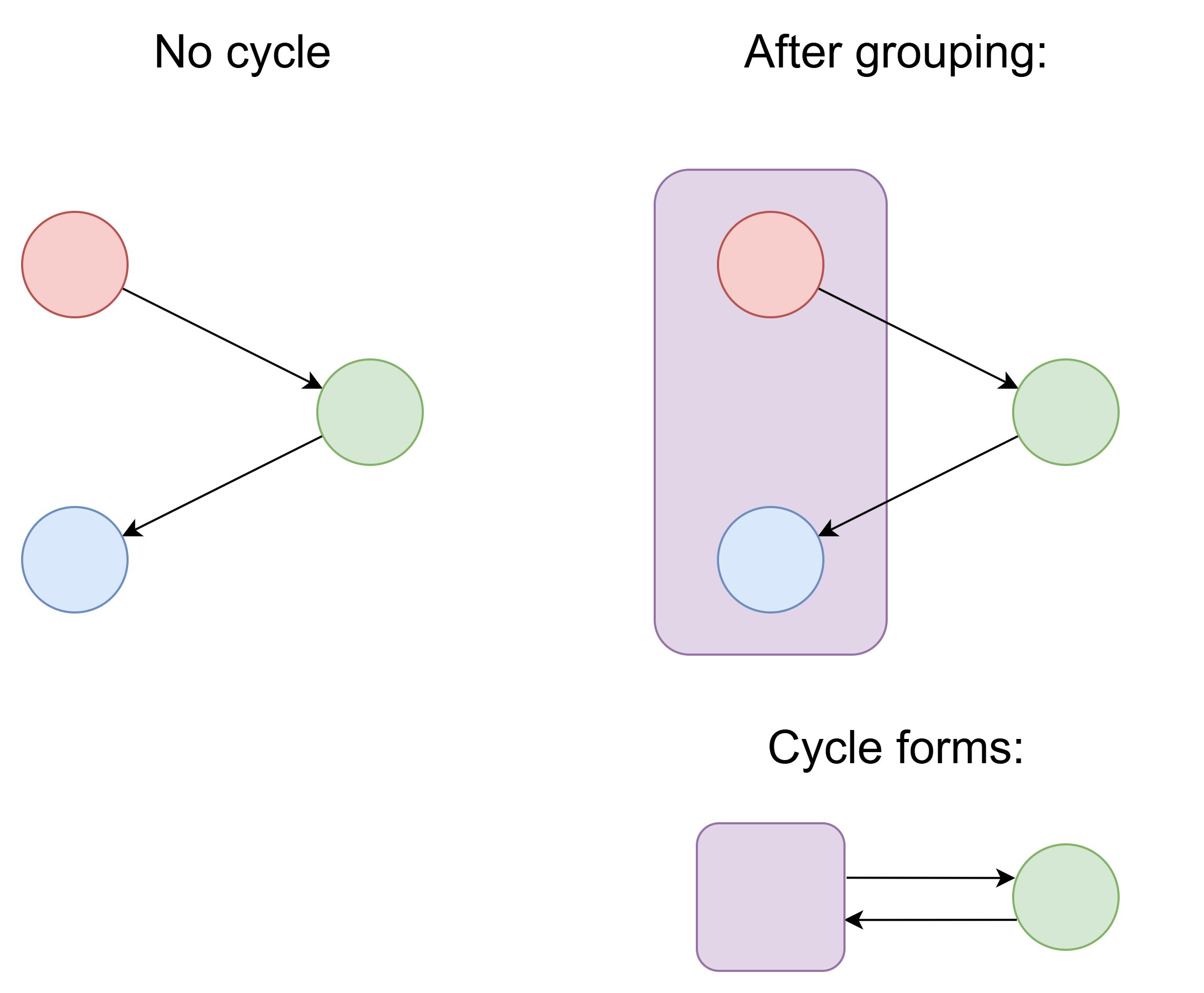
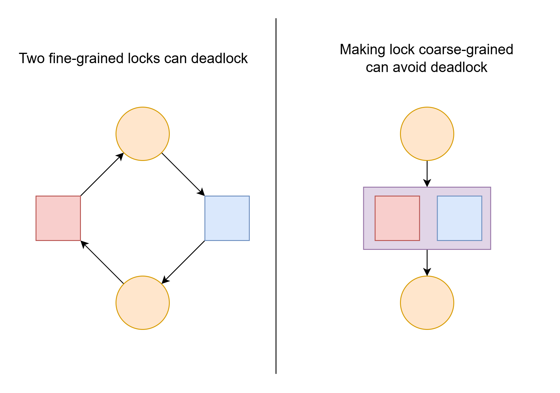
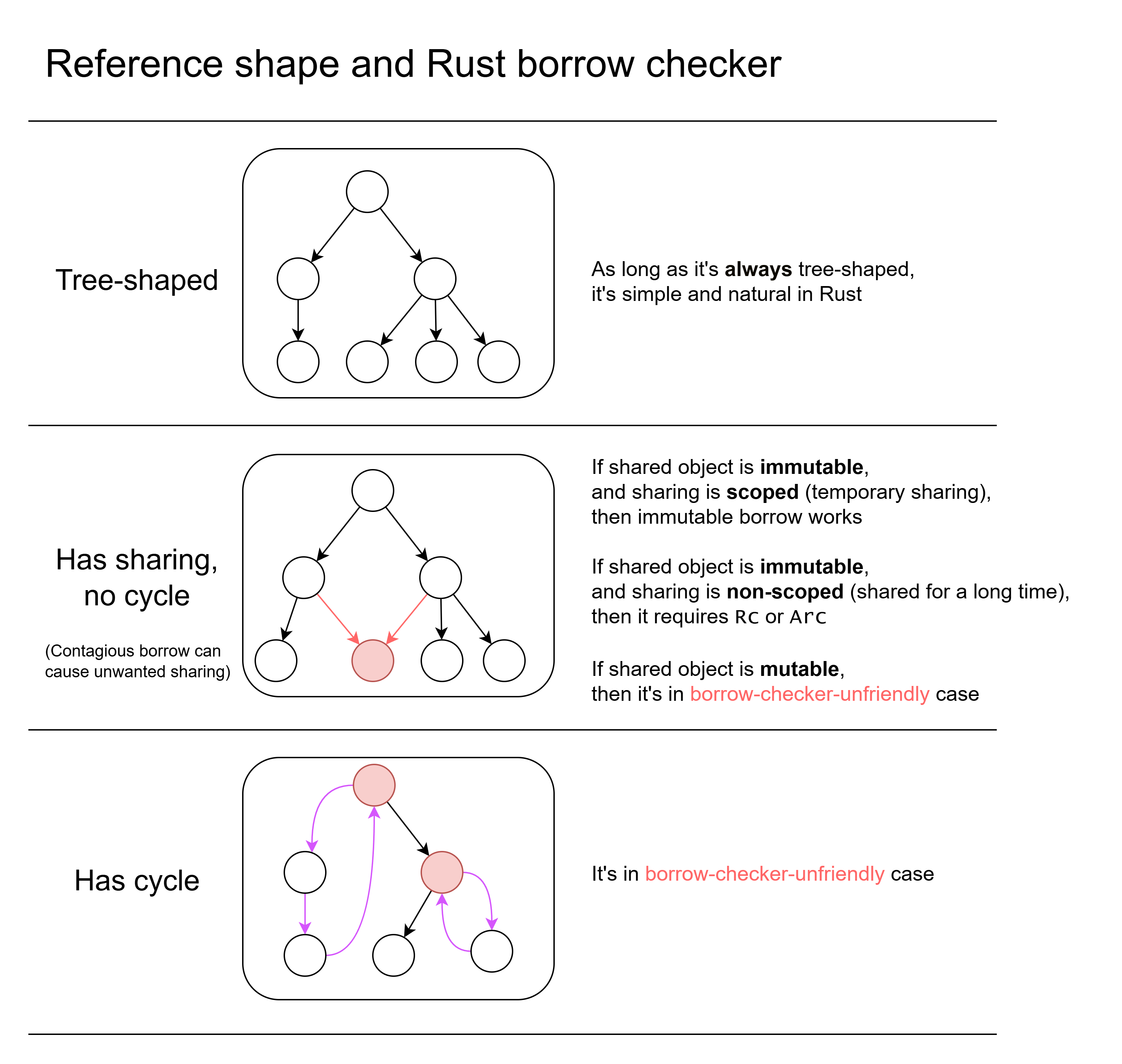
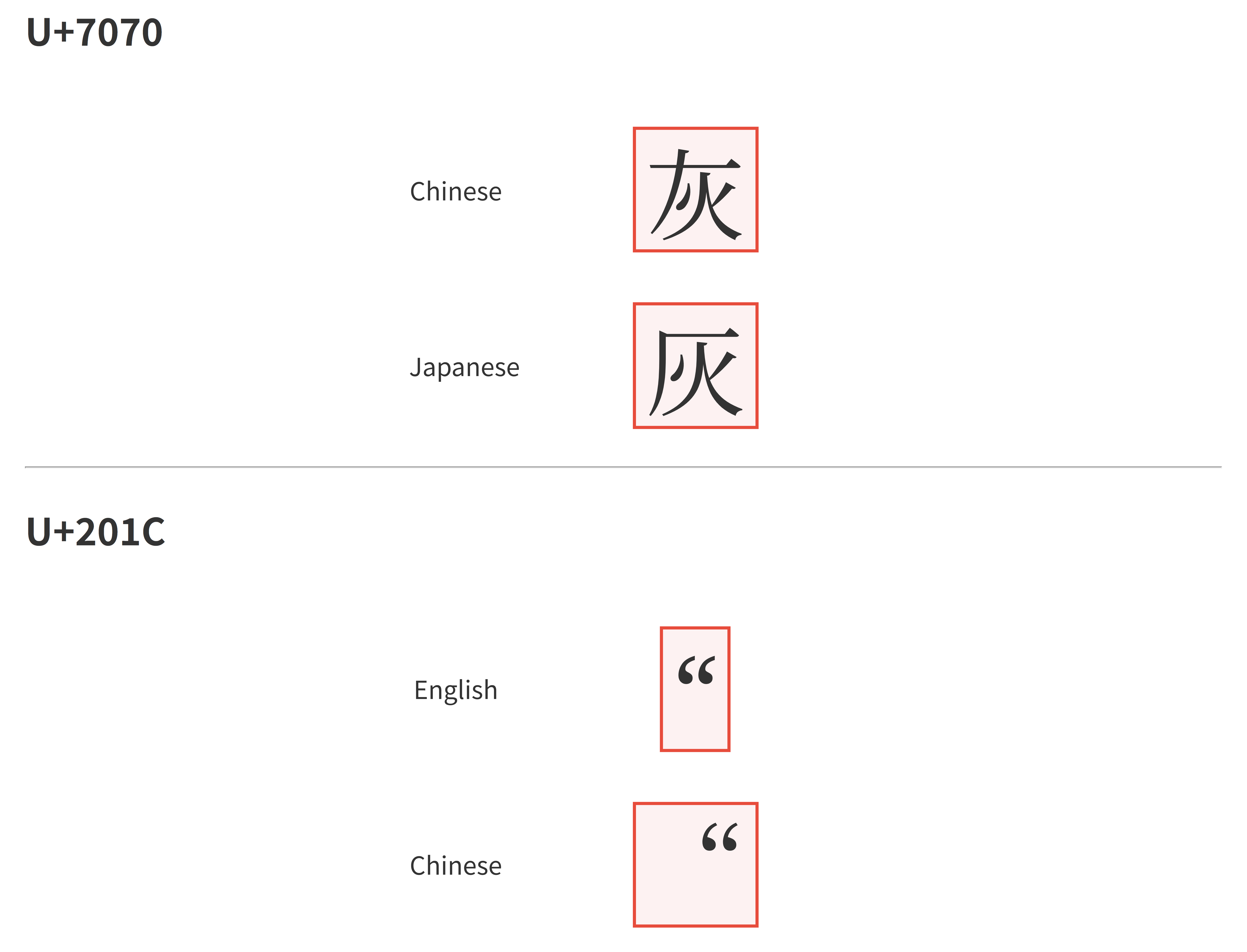
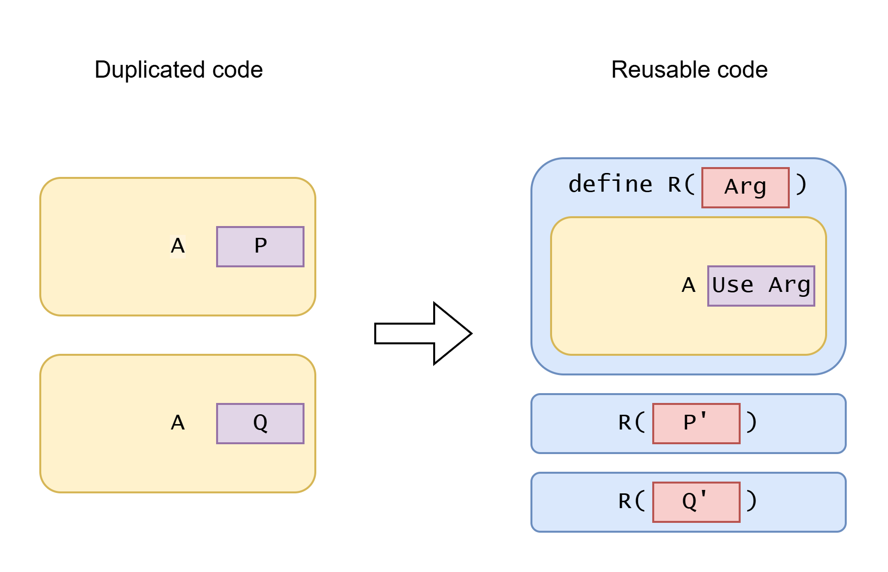
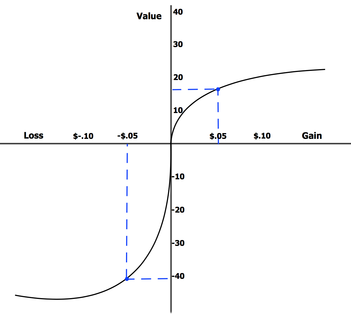
The planes that get hit in critical places never come back, thus don't get included in the stat of bullet holes, forming the regions missing bullet hole in that image.

Other examples of survivorship bias:

Most gamblers are initially lucky, because the unlucky ones tend to quit gambling early.
Assume that many fund managers randomly pick stocks. After one year, some of the lucky ones have good performance, while others are overlooked. In the short term, you cannot know whether success come from just luck.
"Taleb's rat health club": Feeding poison to rats increases average health, because the unhealthy ones are more likely to die from poison.
Social media has more negative news than positive news. Bad news travels fast.
The succeded research results are published and the failed attempts are hidden (P-hacking).
Only special and interesting events appear on news. The more representative common but not newsworthy events are overlooked.
If you analyzed 5 solutions then pickd one solution to present, people think you did little work because they don't see the discarded 4 solutions.

A more generalized version of survivor bias is selection bias: When the sampling is not uniform enough and contains selection mechanism (not necessary 100% accurate selection), there will be bias in the result.

The opinions on social media does not necessarily represent most peoples' view. There are several selection mechanisms in it: 1. not all people use the same social media platform 2. the people using social media may not post opinions 3. not all posted opinions will be seen by you due to algorithmic recommendation.

Some physicists propose Anthropic Principle: the physical laws allow life because the existence of life "selects" the physical law. The speciality of the physical laws come from survivorship bias.

What people don't do is as important as what people do. The negative advices (what not to do) are as important as positive advices (what to do). The experiences of failed ones are also important, not just succeeded ones.

Availability bias

Availability bias: When thinking, the immediate examples that come into mind plays a big role.

Example: If you recently saw a car crash, you tend to think that traveling by car is riskier than traveling by plane. However, if you recently watched a movie about a plane crash, you might feel that planes are more dangerous.

Nothing in life is as important as you think it is when you are thinking about it.

- Daniel Kahnman

Vividness bias: People tend to believe more from vivid things and stories, over abstract statistical evidences. This is related to anecdotal fallacy and narrative fallacy.

The Italian Toddler: In the late 1970s, a toddler fell into a well in Italy. The rescue team could not pull him out of the hole and the child stayed at the bottom of the well, helplessly crying. ...... the whole of Italy was concerned with his fate ...... The child's cries produced acute pains of guilt in the powerless rescuers and reporters. His pictures was prominently displayed on magazines and newspapers .....

Meanwhile, the civil war was raging in Lebanon ...... Five miles away, people were dying from the war, citizens where threatened with car bombs, but the fate of the Italian child ranked high among the interests of the population in the Christian quarter of Beirut.

- The Black Swan

Enforcing safety measures is usually unappreciated. Because people only see the visible cost and friction caused by safety measures (concrete), and do not see the consequences of not applying safety measures in a parallel universe (abstract), until an incident really happens (concrete).

People are more likely to pay terrorism insurance than for plain insurance that covers terrorism and other things.

If people are given some choices, people tend to choose one of the provided choices and ignore the fact that other choices exist. This is also framing effect.

People tend to attribute one product to one public figure, or attribute a company to its CEO, because that's the name that they know, and because of causal simplification tendency.

People often think the quality of new movies/games/novels declines, worse than the ones produced in "golden age" before. However it's mainly due to people only remember good ones and neglect the bad ones filtered by time.

Interestingly, LLMs also seem to have availability bias: the information mentioned before in context can guide or mislead subsequent output. The knowledge that's "implicit" in LLM may be suppressed by context.

When reviewing a document, most reviews tend to nitpick on the most easy-to-understand places, like diagram, or summarization, while not reading subsequent text that explain the nuances.

When judging on other people's decisions, people often just see visible downsides and don't see it's a tradeoff that avoids larger downsides.

Agenda-setting theory: what media pay attention to can influence people's attention, then influence people's opinions.

Saliency bias: We pay attention to the salient things that grab attention. The things that we don't pay attention to are ignored. Attention is a core mechanism of how brain works 5.

"Blind" outside of attention

When people pay attention to one thing, they tend to ignore things that are outside of attention.

Invisible gorilla test: when subject is asked to count things in basketball match, they ignore the special one wearing gorilla suit.

Prior belief (confirmation bias) can affect perception. This not only affects recognition of objects, but also affects reading of text. Under confirmation bias, when reading text, one may skip important words subconsciously.

In software UX: if the user is focused on finishing a task, when the software pops up a dialog, the user tends to quickly close the dialog to continue the task, without reading text in dialog. 6

Anecdotal fallacy

People tend to believe more from stories, anecdotes or individual examples, even if these examples are made up or are just statistical outlier. On the contrary, people are less likely to believe in abstract statistical evidences.

Examples:

"Someone smoked their entire life and lived until 97, so smoking is actually not that bad."
"Someone never went to college and turned out to be successful, so college is a waste of time and money."
"Someone made a fortune trading cryptocurrency, and so can I."
"It was the coldest winter on record in my town this year. Global warming can't be real." 7

Familiarity bias

People prefer familiar things. One reason is the availability bias. Another reason is that people self-justifys their previous attention and dedication. This is highly related to availability bias.

When making decisions, people tend to focus on what they already know, and ignore the aspects that they do not know or are not familiar with. We have already considered what we already know, so we should focus on what we don't know in decision making.

This is related to risk compensation: People tend to take more risk in familiar situations.

Imprinting: At young age, people are more likely to embrace new things. At older age, people are more likely to prefer familiar things and avoid taking risk in unfamiliar things. (Baby duck syndrome).

Anything that is in the world when you’re born is normal and ordinary and is just a natural part of the way the world works.

Anything that's invented between when you’re 15 and 35 is new and exciting and revolutionary and you can probably get a career in it.

Anything invented after you're 35 is against the natural order of things.

- Douglas Adams

Frequency illusion

Noticing something more frequently after learning about it, leading to overestimating its prevalence or importance.

Sometimes, one talked about something then sees its ad in social media, thus suspecting that their phone and social media app is recording voice for ad recommendation. Of course that possibility exists, but perception of that possibility is exaggerated by frequency illusion.

Representativeness bias

People tend to judge things by comparing it with examples (stereotypes) that come into mind, and tend to think that one sample is representative to the whole group.

Representative bias can sometimes be misleading:

Say you had the choice between two surgeons of similar rank in the same department in some hospital. The first is highly refined in appearance; he wears silver-rimmed glasses, has a thin build, delicate hands, measured speech, and elegant gestures. ...

The second one looks like a butcher; he is overweight, with large hands, uncouth speech, and an unkempt appearance. His shirt is dangling from the back. ...

Now if I had to pick, I would overcome my sucker-proneness and take the butcher any minute. Even more: I would seek the butcher as a third option if my choice was between two doctors who looked like doctors. Why? Simply the one who doesn’t look the part, conditional on having made a (sort of) successful career in his profession, had to have much to overcome in terms of perception. And if we are lucky enough to have people who do not look the part, it is thanks to the presence of some skin in the game, the contact with reality that filters out incompetence, as reality is blind to looks.

- Skin in the game

Note that the above quote should NOT be simplified to tell that "the unprofessional-looking ones are always better". It depends on exact case.

Gambler's fallacy

When an event has occured frequently, people tend to believe that it will occur less frequently in the future.

Examples:

When tossing coin, if head appear frequently, people tend to think tail will appear frequently. (If the coin is fair and tosses are statistically independent, this is false. If the coin is biased, it's also false.)
When a stock goes down for a long time, people tend to think it will be more likely to rise.

One related topic is the law of large numbers: if there are enough samples of a random event, the average of the results will converge. The law of large numbers focus on the total average, and does not consider exact order.

The law of large number works by diluting unevenness rather than correcting unevenness. For example, a fair coin toss will converge to 1/2 heads and 1/2 tails. Even if the past events contain 90% heads and 10% tails, this does not mean that the future events will contain more tails to "correct" past unevenness. The large amount of future samples will dilute the finite amount of uneven past samples, eventually reaching to 50% heads.

Actually, gambler's fallacy can be correct in a system with negative feedback loop, where the short-term distribution changes by past samples. These long-term feedback loops are common in nature, such as the predator-prey amount relation. It also appears in markets with cycles. (Note that in financial markets, some cycles are much longer than expected, forming trends.) In a PvP game with Elo-score-based matching mechanism, losing makes make you more likely to win in the short term.

One related concept is regression to the mean, meaning that, if one sample is significantly higher than average, the next sample is likely to be lower than the last sample, and vice versa. Example: if a student's score follows normal distribution with average 80, when that student gets 90 scores, they will likely to get a score worse than 90 in the next exam.

The difference between gambler's fallacy and regression to the mean:

Gambler's fallacy: if the past samples deviate to mean, assume the distribution of future samples change to "compensate" the deviations. This is wrong when the distribution doesn't change.
Regression to the mean: if the last sample is far from the mean, the next sample will likely to be closer to the mean than the last sample. It compares the next sample with the last sample, not the future mean with the past mean.

Regression fallacy: after doing something and regression to the mean happens, people tend to think what they do caused the effect (hasty generalization). Example: the kid gets a bad score; parent criticizes; the kid then get a better score. It's seen that criticizing makes the score get better, although this is just regression to the mean that can happen naturally.

Conjunction fallacy

People tend to think that more specific and reasonable cases are more likely than abstract and general cases.

Consider two scenarios:

A: "The company will achieve higher-than-expected earnings next quarter."
B: "The company will launch a successful new product, and will achieve higher-than-expected earnings next quarter."

Although B is more specific to A, thus have a lower probability than A, people tend to think B is more likely than A. B implies a causal relationship, thus look more reasonable.

People tend to think that a story with more details is more plausible, and treat probability as plausibility. A story with more details is not necessarily more plausible, as the details can be made up.

Making a story more reasonable allows better information compression, thus making it easier to remember and recall.

Curse of knowledge

People often assume that others know what they know. So people often omit important details when explaining things, causing problems in communication and teaching.

When learning a new domain of knowledge, it's beneficial to ask "stupid questions". These "stupid questions" are actually fundamental questions, not stupid at all. But these fundamental questions are seen as stupid by experts, under curse of knowledge.

One benefit of AI is that you can ask "stupid questions" without being humiliated by experts (but be wary of hallucinations).

If a "stupid question" doesn't have a sound answer, then maybe something important is overlooked by everyone.

Simplicity is often confused by familiarity. If one is very familiar with a complex thing, they tend to think that thing is simple.

Curse of knowledge also applies when using AI. If the user assumes AI knows their work detail and don't tell such information to AI, AI tend to output generic useless things. It's recommended to put knowledge of your work (including failed attempts) into a document. It not only reduces your memory pressure but also can be read by AI.

Normalcy bias

Normalcy bias: Thinking that past trend will always continue. This is partially due to confirmation bias.

Although the market has trends, and a trend may be much longer than expected, no trend continues forever. Anything that is physically constrained cannot grow forever.

Most people are late-trend-following in investment: not believing in a trend in the beginning, then firmly believing in the trend in its late stage. This is dangerous, because the market has cycles, and some macro-scale cycles can span years or even decades. The experiences gained in the surge part of the cycle are harmful in the decline part of the cycle and vice versa.

First impression effect (primacy effect)

People tend to judge things by first impression. This makes people generate belief by only one observation, which is information-efficient, but can also be biased.

Recency bias

Overemphasizing recent events, while ignoring long-term trends.

People tend to

overestimate the short-term effect of a recent event, and
underestimate the long-term effect of an old event.

This is related to Amara's law: we tend to overestimate the effect of a technology in the short run and underestimate the effect in the long run.

This is also related to availability bias, where the just-seen events are more obvious and easier to recall than old events and non-obvious underlying trends.

Normalcy bias means underreact to new events, but recency bias means overreact to new events, which is the opposite of normalcy bias. These two are actually not conflicting. Which one takes effect initially is related to actual situation and existing beliefs (confirmation bias). When one person does not believe in a trend but the trend continued for a long time, binary thinking may make that person turn their belief 180 degrees and deeply believe in the trend.

Relation between recency effect and primacy effect:

One firstly sees A, then after a long time, then sees B, recency effect tells that B has higher influence than A.
One firstly sees A, then sees B, then after a long time, primacy effect tells A has higher influence than B.

Framing effect

People tend to make decisions based on how information is presented (framed) rather than objective facts.

There are many ways to frame one fact. For example, one from positive aspect, one from negative aspect:

"90% of people survive this surgery" / "10% of people die from this surgery".
"99.9% effective against germs" / "Fails to kill 0.1% of germs".
"You are the hero of your own story" / "No one is coming to help you".

The wording of a thing can affect how people perceive it. Examples:

"Gun control" / "Gun safety"
"Government subsidy" / "Using taxpayer money"
"Risk measurement" / "Risk forecast"
"Necessary trade-off" / "Sacrifice"
"Flood of refugees" / "Exodus"
"Be rejected" / "Dodged a bullet"

The content creator could emphasize one aspect and downplay another aspect, and use different wording or art style to convey different opinions. The people reading the information could be easily influenced by the framing subconsciously.

A loaded question is a question that contains an assumption (framing). Following that assumption can lead to a biased answer. Example: "Do you support the attempt by the US to bring freedom and democracy to other places in the world?"

The current LLMs are mostly trained to satisfy the user. If you ask LLM a loaded question that has a bias, the LLM often follow your bias to please you.

Asking the right question requires the right assumption.

Mehrabian's rule: When communicating attitudes and feelings, the impact is 7% verbal (words), 38% vocal (tone of voice), 55% non-verbal (facial expressions, gestures, posture). Note that this doesn't apply to all kinds of communications.

Just looking confident can often make other people believe. This even applies when the talker is AI:

A friend sent me MRI brain scan results and I put it through Claude. No other AI would provide a diagnosis, Claude did. Claude found an aggressive tumour. The radiologist report came back clean. I annoyed the radiologists until they re-checked. They did so with 3 radiologists and their own AI. Came back clean, so looks like Claude was wrong. But looks how convincing Claude sounds! We're still early...

- Link

Anchoring bias: People's judgement may be influenced by reference "anchors", even if the reference anchor is irrelevant to decision making. Anchoring is a kind of framing. A salesman may firstly show customers an expensive product, then show cheap products, making customers feel the product being cheaper, utilizing anchoring bias.

The Anchoring Bias and its Effect on Judges.

Decoy effect: Adding a new worse option to make another option look relatively better.

Lie by omission: A person can tell a lot of truth while omitting the important facts, stressing unimportant facts (wrong framing), intentially causing misunderstanding, but at the same time be not lying in literal sense.

Sometimes an example or a diagram can be misleading, due to lie by omission. If there are 2 possible cases, but the diagram only draw first case, then the diagram viewer may subconciously ignore possibly of the second case.

The price chart is often drawn by making lowest price at the bottom and highest price at the top. The offset and scale of the chart is also framing. If one stock already have fallen by 30%, the latest price is in the bottom of the chart, so the stock seems cheap when looking at the chart, but it may actually be not cheap at all, and vice versa.

Reversal of burden of proof: One common debating technique is to reverse the burden of proof to opponent: "My claim is true because you cannot prove it is false." "You are guilty because you cannot prove you are innocent."

PowerPoint (keynote, slide) medium is good for persuading, but bad for communicating information. PowerPoint medium encourages author to omit imformation instead of writing details. Amazon bans PowerPoint for internal usage. See also: Columbia Space Shuttle Disaster, Military spaghetti powerpoint.

Analogies also utilize framing bias. For example: "National deficit is like a credit card bill" / "National deficit is like a business investment".

Some media often do quoting out of context (断章取义). Natural language is often vague and the meaning highly depends on context. Removing context can easily cause misleading understanding. This also utilizes framing bias.

Two talking styles

Two different talking styles: the charismatic leader one and the intellectual expert type:

Charismatic leader talking styleIntellectual expert talking styleConfident and assertive. (doesn't fear of being wrong)Conservative and rigorous. (fear of being wrong)Persuades using narratives and emotions (more effective to most people)Persuades using expert knowledge and evidence (less effective to most people)Create hope and missionWarn about tradeoffs and possible risksOften take risk and bear responsibility. Often make decisions quickly using intuition and simple logicOften conservative and hesitate in taking risk and bearing responsibility

Note that the above are two simplified stereotypes. The real cases may be different.

Related: A good leader should be insistent when the leader is sure it's correct. A good leader should be open-minded when not sure. A bad leader pretends to be nice when knowing sure it's wrong. A bad leader become insecurely aggressive when being challenged for things the leader is not sure.

Blame the superficial

"Shooting the messenger" means blaming the one who bring the bad news, even though the messenger has no responsibility of causing the bad news.

The same effect happens in other forms:

Blaming the journalist exposing the bad things in society.
Refuse medical treatment, because medical treatment reminds illness and show weakness.
In corporation, the responsibility of solving a problem usually belongs to the one raising the problem, not the one creating the problem.

Imagine someone who keeps adding sand to a sand pile without any visible consequence, until suddenly the entire pile crumbles. It would be foolish to blame the collapse on the last grain of sand rather than the structure of the pile, but that is what people do consistently, and that is the policy error. ...

As with a crumbling sand pile, it would be foolish to attribute the collapse of a fragile bridge to the last truck that crossed it, and even more foolish to try to predict in advance which truck might bring it down. ...

Obama’s mistake illustrates the illusion of local causal chains - that is, confusing catalysts for causes and assuming that one can know which catalyst will produce which effect.

- The Black Swan of Cairo; How Suppressing Volatility Makes the World Less Predictable and More Dangerous

Scarcity heuristic

People tend to value scarce things even they are not actually valuable and undervalue good things that are abundant.

Examples:

When an online learning material is always there, people have no pressure to learn and often just bookmark it.
A thing that's sold in a time-limited or amount-limited way is deemed to be valuable.
Restrict buying something make people buy it more eagerly even when they don't need that thing. Same as restricting some information may increase people's perceived value of that information.

People tend to value something only after losing it.

Health is forgotten until it’s the only thing that matters.

- Bryan Johnson, Link

Simpson's paradox and base rate fallacy

The correlation of overall samples may be contradictory to the correlation inside each sub-groups.

Reference

Examples:

In the COVID-19 pandemic, a developed country have higher overall fatality rate than a developing country. But in each age group, the developed country's fatality rate is lower. The developed country has a larger portion of old population.
After improving a product, the overall customer satisfaction score may decrease, because the product gets popular and attracted the customers that don't fit the product, even though the original customers' satisfaction score increases.
You post on internet something that 90% people like and 1% people hate. The people liking the post usually don't direct-message you. But the people hating it often have strong motivation to direct-message you. So your direct message may contain more haters than likers, even though most people like your post.

Base rate fallacy: there are more vaccinated COVID-19 patients than un-vaccinated COVID-19 patients in hospital, but that doesn't mean vaccine is bad:

Reference

In these cases, confounding variable correspond to which subgroup the sample is in. Statified analysis means analyzing separately in each subgroup, controlling the confounding variable.

False consensus (echo chamber, information cocoon)

When one person is in a small group with similar opinions, they tend to think that the general population have the similar opinions. When they encounter a person that disagrees with them, they tend to think the disagreer is minority or is defective in some way.

This effect is exacerbated by algorithmic recommendation of social medias.

We also tend to think other people are similar to us in some ways. We learn from very few examples, and that few examples include ourselves.

We don't see things as they are. We see things as we are.

Priming

We use relations to efficiently query information in memory. The brain is good at looking up relations, in an automatically, unintentionally and subconscious way.

Being exposed to information makes human recognize similar concepts quicker. Examples:

Reminding "yellow" makes recognizing "banana" faster.
Reminding "dog" makes recognizing "cat" faster.

Being exposed to information also changes behavior and attitudes. Examples:

Being more likely interpret things as danger signals after watching a horror movie.
Red in food packaging increases people's intention to buy it.
Being familiar with a brand after exposed to its ads, even after trying to ignore ads.
Sleeper effect: After exposed to persuation, people that don't initially agree may gradually agree after time passes.

The main moral of priming research is that our thoughts and our behavior are influenced, much more than we know or want, by the environment of the moment.

- Think, fast and slow

Note that the famous "age priming" effect (walk more slowly after reminding aging concepts) failed to be replicated.

The placebo effect is also possibly related with priming.

Slot machines have a mechanism: losses disguised as wins (LDWs). When gambler wins, the machine shows fancy lights and plays sounds, stimulating the gambler. But when the gambler slightly losses, the machine still give light and sound stimulus, creating a feeling of win. Then gambler then feels win more than actual wins.

Spontaneous trait transfer: listeners tend to associate what the talker say to the talker, even when talker is talking about another person:

If you praise another person, the listeners tend to subconsciously think that you are also good.
If you say something bad about another person, the listeners tend to subconsciously think you are also bad.

Flattering subconsciously increase favorability, even when knowing it's flattering (this even applies to sycophant AI). Saying harsh criticism subconsciously reduce favorability, even when knowing the criticism is beneficial. Placebo still works even when knowing it's placebo.

Efficient decision making

When making decisions, human tend to follow intuitions, which is quick and energy-efficient, but also less accurate.

Often quickly making decision before having complete information is better than waiting for complete investigation.
Sometime multiple decisions both can fulfill the goal. The important is to quickly do action, rather than which decision is optimal.

Thinking, Fast and Slow proposes that human mind has two systems:

System 1 thinks by intuition and heuristics, which is fast and efficient, but inaccurate and biased.
System 2 thinks by rational logical reasoning, which is slower and requires more efforts, but is more accurate.

Most thinking mainly uses System 1 while being unnoticed.

Emotion overrides rationality

With intense emotion, the rationality (System 2) is being overridden, making one more likely to make mistakes.

Some examples:

When being criticized, the more eager you are trying to prove you correct, the more mistake you may make.
The trader experiencing loss tend to do more irrational trading and lose more money.

Being calm can "increase intelligence".

When one is in intense emotion, logical argument often has little effect in persuading, and emotional connection is often more effective.

Default effect

People tend to choose the default and easiest choice. Partially due to laziness, partially due to fear of unknown risk.

In software product design, the default options in software plays a big role in how user will use and feel about the software. Increasing the cost of some behavior greatly reduces the people doing that behavior:

If a software functionality require manually enabling it, much fewer users will know and use that functionality.
Just 1 second longer page load time may reduce user conversion by 30%. Source
Each setup procedure will frustrate a portion of users, making them give up. A good product requires minimal configuration to start working.

Sometimes, if doing something is 10% more difficult, then 50% fewer people will do it, vice versa. It's non-linear.

Ask for no, don’t ask for yes. When asking others to approve something they didn't plan, they tend to not approve or delay approving, as the approver bears responsibility. Just proceed by default and ask for no holds more control and bears more responsibility.

Software UX design should avoid confronting user with a must-be-made decision. Making decision consumes mental efforts and gives feeling of risk. The software should have a reasonable default and let user to customize on demand.

Status quo bias: tend to maintain status quo. This is related to risk aversion, as change may cause risk.

A related concept is omission bias: People treats the harm of doing something (commision) higher than the harm of not doing anything (omission). Doing things actively bears more responsibility. In the trolley problem, not doing anything reduces perceived responsibility.

If there is an option to postpone some work, the work may eventually never be done.

Path dependence: sticking to what worked in the past and avoid changing, even when the paradigm has shifted and the past successful decisions are no longer appropriate.

I think people's thinking process is too bound by convention or analogy to prior experiences. It's rare that people try to think of something on a first principles basis.

They'll say, "We'll do that because it's always been done that way." Or they'll not do it because "Well, nobody's ever done that, so it must not be good."

But that's just a ridiculous way to think.

You have to build up the reasoning from the ground up - "From the first principles" is the phrase that's used in physics. You look at the fundamentals and construct your reasoning from that, and then you see if you have a conclusion that works or doesn't work, and it may or may not be different from what people have done in the past.

- Elon Musk

Law of the instrument: "If the only tool you have is a hammer, it is tempting to treat everything as if it were a nail."

We shape our tools, and thereafter our tools shape us.

Action bias

Action bias: In the places where doing action is normal, people prefer to do something instead of doing nothing, even when doing action has no effect or negative effects.

When being judged by other people, people tend to do action to show their value, productivity and impression of control:

A personal doctor may do useless medications to show they are working. (Antifragile argues that useless medications are potentially harmful. It's naïve interventionism.)
A politician tend to do political action to show that they are working on an affair. These policies usually superficially helps the problem but doesn't address the root cause, and may exacerbate the problem. One example is to subsidize house buyers, which makes housing price higher, instead of building more houses.
Financial analysts tend to give a definitive result when knowing there isn't enough sound evidence.

For high-liquidity assets (e.g. stocks), people tend to do impulsive trading when market has volatility. But for low-liquidity harder-to-trade assets (e.g. real estate) people tend to hold when the market has volatility.

Action bias does not contradict with default effect. When one is asked to work and show value, doing action is the default behavior, and not doing action is more risky, as people tend to question the one that does not look like working.

It's not the things you buy and sell that make you money; it's the things you hold.

- Howard Marks

Also, when under pressure, people tend do make actions in hurry before thinking, which increase the chance of making mistakes.

Prioritizing the easy and superficial

Law of least effort: people tend to choose the easiest way to do things, choosing path of least resistance. 8

Some seemingly easy solutions do not address the root cause, having negligible effect or negative effect in the long run. Applying the easy solution gives the fake impression that the problem is being addressed, achieving mental comfort.

Examples:

Focusing on buying exercise equipments instead of exercising. Paying to gym without going to gym.
Buying supplements instead of adopting healthier lifestyle.
Focusing on buying courses, books, study equipments instead of actually studying. Keep bookmarking online learning materials instead of reading them.
Musicians focusing on buying instruments (gear acquisition syndrome).
A manager pushing employees to seemingly work hard instead of improving efficiency.
A parent train child by punishing hard, instead of using scientific training methods.
Bikeshedding effect: during meetings, people spend most time talking about trivial matters.
Staying in comfort zone. Only learn/practice the familiar things and avoid touching unfamiliar things. Avoiding the unpleasant information when learning.
Only care about the visible numbers (KPI, OKR), and ignore the important things behind the numbers, like perverse incentives caused by the KPI, statistical bias, and the non-measurable things.
Streetlight effect: Only search in the places that's easy to search, not the places that the target is in.
Hiding the signal of error instead of diagnosing and solving the error.

This is related to means-end inversion. To achieve the root goal (end) we work on a sub-goal (means) that helps root goal. But focusing on an easy but unimportant sub-goal may hurt the root goal, by taking resources from hard but important sub-goals.

A similar phenomenon occurs commonly in medicine: treatments usually mainly suppress superficial symptoms (e.g. painkiller) instead of curing the root cause of illness. This is usually due many other factors.

Pepole tend to spend much time making decision on small things but spend very few time making decisions on big things (e.g. buy house with mortgage, big investment):

As the big decision is important, people tend to be nervous when thinking about it.
Thinking about big decisions is tiresome, as the future is uncertain, and there are many factors to analyze.
So people tend to procrastinate to avoid the unpleasant feeling of thinking about big decisions, or simply follow others (herd metality).
The small decisions (e.g. choosing item in shop, choosing restaurant) require less mental efforts and cause less nervous feeling. Thinking on these decisions can give feeling of control. These decisions usually have quick feedback (human crave quick feedback).

Herd mentality

One easy way to make decisions is to simply follow the people around us. This is beneficial in ancient world: for example, if a tiger comes and some people start fleeing, following them is better than spending time recognizing the tiger.

Social proof heuristic: Assuming that surrounding people know the situation better, so following them is correct.

Following the crowd is also a great way of reducing responsibility: when everyone is guilty, the law cannot punish everyone. The one that acts independently bears more responsibility (omission bias). People often fear of acting independently.

Worldly wisdom teaches that it is better for reputation to fail conventionally than to succeed unconventionally.

- John Maynard Keynes

When the whole group makes a mistake, the sin of the whole group tend to transfer to a scapegoat, then punish the scapegoat. 9

When many people follow each other, they will confirm each other, creating self-reinforcing feedback loop. This is also a reason of the momentum in markets. People tend to be overconfident when people around them are confident, and vice versa.

Two kinds of knowing:

I know something. But I am not sure other people also know it. Other people may also be not sure I know it. There is no consensus even if everyone thinks the same. This is pluralistic ignorance. It can happen when there is taboo that prevents communicating that information.
I know something. I also know other people also know it. I also know other people know me know it. It's common knowledge. This is the kind of knowledge that drives herd mentality.

In "The emperor's new cloth" story, "king is clothless" is originally not common knowledge, even though everyone knows. But once the child states the truth publicly, that knowlege becomes common knowledge.

The forming of new common knowledge is often self-reinforcing feedback loop. Once the momentum forms, it can unleash big power.

Herd mentality can cause self-fulfilling prophecy. This is common in market: if many people expect one thing's price will grow, then people tend to buy it now, then its price do grow, vice versa.

Price grow often depends on "delta" of believers, instead of the existing believers.

Veblen good: higher price induce more demand, unlike normal commodity.

Measuring people's belief by observing the people around you is inaccurate, because the people near you don't necessarily represent all people (representative bias).

Herd mentality is in some sense a kind of trend following strategy. If the trend is some new good technology then following is good regardless of early or late. However, for speculative financial assets, the price grow depends on new people and money entering, so most people will start following too late and cannot profit from it.

One similar effect, in-group bias: Favoring investments or opinions from people within one's own group or those who share similar characteristics.

Bystander effect: People are less likely to help a victim in the presence of other people.

Mimetic desire: We tend to pursue for thing that other people pursue, not based on personal perferences.

Pack journalism: When journalists communicate together, their views tend to converge to the same.

"Because" justification

In an experiment, requesting jumping the queue of using a copy machine:

RequestAccept rate"... May I use the Xerox machine?"60%"... May I use the Xerox machine because I have to make some copies?"93%"... May I use the Xerox machine because I’m in a rush?"94%

Providing a non-reasonable reason "because I have to make some copies" also increases accept rate similar to a normal reason.

Mental accounting

Mental accounting: Treating different parts of money differently, based on their source or intended use.

For example, one can separate the budgets for entertainment, housing and food. It's a simple huristic that can avoid excessive spending: if each part doesn't overspend, then they won't overspend overall.

Mental accounting is related to sunk cost and loss aversion. If one sub-account is low, people tend to be more saving in that sub-account, making loss aversion more significant, and the previous waste in that sub-account become sunk cost.

In investment, mental accounting can happen on different forms:

Seperate by different time intervals. Setting profit target in each time interval (by month, season or year) can be detrimental in a market with momentum. If the profit in the time interval is meet, stop investing misses large profit from trend. If the profit in the time interval is not meet near the end, then the trader tend to be more nervous and more aggressive, which is dangerous.

However, setting stop-loss in each time interval may be good. When the current trading strategy does not fit the market, temporarily stopping could get through the current part of cycle that temporarily doesn't suit the strategy. The stopping period also helps calm down and become rational.
Separate by different specific assets (e.g. stocks). If the mental accounts are separated based on different stocks, after losing from one stock, one may insist to gain the loss back from the same stock, even if investing in other stocks is better overall.
Separate by different categories of assets. People tend to prefer investing medium risk asset using all money over investing high-risk asset using partial money (barbell strategy), even when the total volatility and expected return are the same, because the invested money is in a different mental account than not-invested money, and risk aversion.

Lipstick effect is related to mental accounting. When the income declines, the mental account of luxury spending still exists, just shrunk, so cheaper lipsticks get more sales.

Mental accounting is one kind of narrow framing bias:

Narrow framing bias and zero-risk bias

Narrow framing bias: focusing too much on one aspect while neglecting other aspects.

Zero-risk bias: preferring to eliminate one type of risk entirely rather than reducing overall risk (usually at the expense of increasing exposure to other risks).

It's related to binary thinking: thinking that a risk is either completely eliminated or not being taken any action on.

Examples:

Enforcing extreme lockdown to eliminate the risk of a pandemic, causing more risk in other diseases (because hospitals are locked down) and more risk in basic living (food supply is constrainted due to extreme lockdown).
Wanting to hedge inflation by heavily investing in risky assets, whose risk can be higher than inflation. In a liquidity crisis, cash is more valuable than assets.

It should NOT be simplified to "avoiding risk is bad". The point is to not do extreme tradeoffs to eliminte one kind of risk but increase exposure to other kinds of risks.

Regret aversion

People tend to avoid regret. Regret aversion has two aspects:

For future: people tend to avoid making decisions that may cause regret in the future. This is related to risk aversion: not making optimal decision is also a kind of risk.
For past: people tend to avoid regretting their past actions, trying to prove the correctness of their past actions, thus fall into sunk cost fallacy.

The world is full of randomness. There is no decision that guarantees to be optimal. We should accept that we cannot always make perfect decisions. Validating the strategy in the long run is more important than result in of individual decisions.

We tend to regret doing something in short term, but regret not doing something in the long term. Reference.

'I have led a toothless life', he thought. 'A toothless life. I have never bitten into anything. I was waiting. I was reserving myself for later on - and I have just noticed that my teeth have gone. ...'

- Jean-Paul Sartre

Some decisions are consequential and irreversible or nearly irreversible – one-way doors – and these decisions must be made methodically, carefully, slowly, with great deliberation and consultation. If you walk through and don’t like what you see on the other side, you can’t get back to where you were before. We can call these Type 1 decisions.

But most decisions aren’t like that – they are changeable, reversible – they’re two-way doors. If you’ve made a suboptimal Type 2 decision, you don’t have to live with the consequences for that long. You can reopen the door and go back through. Type 2 decisions can and should be made quickly by high judgment individuals or small groups.

As organizations get larger, there seems to be a tendency to use the heavy-weight Type 1 decision-making process on most decisions, including many Type 2 decisions. The end result of this is slowness, unthoughtful risk aversion, failure to experiment sufficiently, and consequently diminished invention.

- Jeff Bezos

Forgive yourself for not knowing earlier what only time could teach.

The more non-trivial things you do, the more mistakes you will make. No one can make no mistake when doing non-trivial things. However, company KPIs often have large weight on punishing mistakes (loss aversion). This cause veteran employees learn to be overly conservative, resulting in lower competitiveness of the whole company.

Risk compensation

Having safety measures make people feel safer and take more risks.

For example, drivers may drive faster when safety belt is on, and cyclists may ride faster when wearing helmet.

People tend to be overconfident in familiar situations, but that's where accidents are likely to occur:

Most accidents (69%) occurred on slopes that were very familiar to the victims. Fewer accidents occurred on slopes that were somewhat familiar (13%) and unfamiliar (18%) to the victim.

- Evidence of heuristic traps in recreational avalanche accidents

Stress and fight-or-flight

"Fight or flight" are the two options for dealing with physical threat (e.g. a tiger) in the ancient world.

But in the modern world, there are non-physical threats and modern risks (e.g. exam failure, losing job). These modern threats can be dealt with neither concrete fight or flight. So they may cause depression, anxiety and immobilization.

Cortisol is a kind of hormone that's correlated with stress. Cortisol has many effects, like making you more vigilent and less relax. If the cortisol level keeps being high for long time, there will be health issues like weight gain, weakened immune system, sleep deprivation, digest issues, etc.

From evolutionary perspective, cortisol system makes one more likely to survive under physical threats (e.g. a tiger) at the expense of other aspects. These physical threats are usually quick and short (e.g. either die or flee from tiger). But the modern risks are usually long and chronic (e.g. worry about exam several months before exam, worry about paying mortgage every day), so that cortisol system is not adaptive.

Also, after seeing a post on social media that cause anger, the cortisol increases and enters nervious mode. Then even after blocking the author and hiding the post, one is still in nervous mode. The nervousness will keep one thinking about the post and/or keep gathering information which is to continue browsing social media.

Willpower and mental energy

The rational activities (System 2 activities) require mental energy (willpower):

Resisting impulse behavior consumes willpower (e.g. resist eating sweet food when on a diet).
Paying attention and thinking hard problems consume willpower.
For introverts, social interaction consumes willpower. But for extroverts, staying alone consumes willpower.

If there is no enough mental energy, one is less likely to resist impulse behaviors or think about hard problems, and possibly have difficulty in social interactions. 10

These factors affect mental energy:

Sleeping and mental resting can replenish mental energy.
Body conditions (like blood sugar level 11) affects mental energy.
Exercising self-control can strengthen mental energy, similar to muscular strength.
Lingering emotion (e.g. keep ruminating past mistakes) costs mental energy.

Mental resting is different to body resting. Intense thinking when lying on the bed even consumes mental energy. Mental resting involves focusing on simple things with low cognitive demand.

Before you try to increase your willpower, try to decrease the friction in your environment.

- James Clear, Link

For normal people, doing a task consumes willpower. But if one loves doing the task, then one gains willpower instead of consuming when doing the task. It's a big advantage.

Memory distortion

In the process of self-justification, people's memory may be distorted. Human memory is actually very unreliable. People usually cannot notice that their memory has been distorted, and insist that their memory is correct.

People tend to simplify their memory and fill the gaps using their own beliefs. This is also an information compression process, at the same time producing wrong memory and biases.

Memorizing is lossy compression. Recall is lossy decompression, where details can be made up in a congruent way. Each recall can reshape the memory according to the existing beliefs. (This is similar to quantum effects: if you observe something, you change it.)

I have a pet theory that when people introspect about themselves, their brain sometimes just scrambles to generate relevant content. So they feel like they're gaining insight into deeper parts of themselves when they're actually just inventing it on the fly.

- Amanda Askell, Link

Information is costly to store, and even more costly to index and query. Sometimes forgetting is just not being able to query the specific memory that is stored in brain (and may be recalled if some cue were found that enables querying it). The "querying capacity" of brain is limited and can be occupied by distracting things. 12

Taking notes is one way to mitigate the unreliable memory issue.

Every time a messsage is relayed through a person, some of its information gets lost, and some noise gets added. The person relaying the message will add their own understanding (which can be misleading), and omit the information that they think is not important (but can be actually important). This issue is very common in big corporation and governments. Good communication requires reducing middlemen.

People usually remember the "special" things well. This is an information compression mechanism that filters out the unimportant details.

Peak-end rule: People judge an experience largely based on how they felt at its peak (its most intense point) and at its end. The most efficient way to improve user experience is to improve the experience in the peak and in the end.

Serial position effect: people tend to recall the first and last items best, and the middle items worst. Interestingly, the same effect also applies to LLMs, called "lost in the middle".

Cryptomnesia: Treating other peoples' idea as own original idea, after forgetting the source of the idea.

Sleeper effect: After exposed to persuation, some people initially don't agree because of some reasons. But after time passes, people may forget the reasons why they initially disagree, and may gradually agree to it. Persuations that don't work immediately may still have long-term effects.

Information addiction and curiosity

People seek information that they are interested in. The seeking of interesting information drives both curiosity and information addiction.

As with food, we spent most of our history deprived of information and craving it; now we have way too much of it to function and manage its entropy and toxicity.

- N. N. Taleb, Link

Most information in the world is junk.

The best way to think about it is it's like with food. There was a time, like centuries ago in many countries, where food was scarce, so people ate whatever they could get, especially if it was full of fat and sugar. And they thought that more food is always good. ...

Then we reach a time of abundance in food. We have all these industrialized processed food, which is artificially full of fat and sugar and salt and whatever. It was always been for us that more food is always good. No, definitely not all these junk food.

And the same thing has happend with information. Information was once scarce. So if you could get your hands on a book you would read it, because there was nothing else.

And now information is abundant. We are flooded with information, and much of it is junk information, which is artificially full of greed, anger and fear, because of this battle for attention.

It's not good for us. We basically need to go on an information diet. Again the first step is to realize that it's not the case that more information is always good for us. We need a limited amount. And we actually need more time to digest the information. And then we have to be of course also careful about the quality of what we take in, because of the abundance of junk information.

The basic misconception I think is this link between information and truth. The people think "ok if I get a lot of information, this is the raw material of truth, and more information will mean more knowledge". That's not the case. Even in nature more information is not about the truth.

The basic function of information in history, and also in biology, is to connect. Information is connection. And when you look at history you see that, very often, the easiest way to connect the people is not with the truth. Because truth is a costly and rare kind of information. It's usually easier to connect people with fantasy, with fiction. Why? Because the truth tends to be not just costly, truth tends to be complicated, and it tends to be uncomfortable and sometimes painful.

In politics, a politician who would tell people the whole truth about their nation is unlikely to win the elections. Every nation has these skeleton in the cupboard, all these dark sides and dark episodes that people don't want to be confronted with.

If you want to connect nations, religions, political parties, you often do it with fiction and fantasies.

- Yuval Noah Harari, Link

Information bias: Seeking out more information even when more information is no longer useful.

With confirmation bias, more information lead to higher confidence, but not better accuracy. This is contrary to statistics, where more samples lead to more accurate result (but still suffer from systematic sampling bias).

Read a lot? No. Be very, very selective & vigilant.

Promiscuous reading destroys one's noise-signal detector, causes atrophy of critical thinking skills.

- N. N. Taleb

Having no information is better than having wrong information. Wrong information reinforced by confirmation bias can make you stuck in a wrong path.

Popularity of false information increase the value of true information. The best way of hiding something is to override it with another thing.

Browsing social media makes people learn biased distribution of world. Such as:

Overestimating the amount of perfect partners, who are beautiful/handsome, have high income and does exaggeraged love.
Believing in false consensus, the consensus that only exists on an internet community.
Overestimating the proportion of bad news, as bad news travels fast in social media, thus facilitating cynicism.

The 80/20 rule also applies to social media: most (e.g. 80%) voice come from few (e.g. 20%) of users. The dominant narrative on internet may not represent most people's views.

What's more, social media may make people:

Get used to interesting easy-to-digest information and become less tolerant to not-so-interesting hard-to-digest information.
Get used to moving attention (distraction) and not get used to keeping attention. In social media, different posts are usually irrelevant and understanding them requires moving attention (forget previous context).
Have less intention of trying things via real world practice. Watching videos about a new experience is much easier than experiencing in real life.

Getting information from real practice is often better than keep browsing information from internet.

Two different kinds of information consumption: long-attention and short-attention:

Long-attentionShort-attentionExample in text: Reading long novelExample in text: Browsing X(Twitter)Example in video: Watching movieExample in video: Wathing TikTokNext content is highly relevant to previous contentNext content is likely irrelevant to previous contentBrain needs to remember previous context to better understand next contentBrain needs to ignore previous context to better understand next contentPractices keeping attentionPractices moving attention Natural selection of memes

Note that "meme" here generally means the information that spreads itself, not limited to entertainment internet memes.

Social medias are doing "natural selection" to memes. The recommendation algorithm makes the posts that induce more interactions (likes and arguing) more popular. It selects the memes that are good at letting human to spread them.

What memes have higher ability to spread?

Induce anger. Saying an idea that you want to refute.
Induce superiority satisfaction.
Express existing thoughts. Utilizes confirmation bias.
Simple and easy-to-understand.
Looks convincing and reasonable. Utilizes narrative fallacy.
Exaggerated. Polarized. Utilizes binary thinking.
Providing interesting new information. Utilizes information addiction.

In the ancient world, when there was no algorithmic recommendataion, there was still the "natural selection" of memes (stories, cultures) but slower.

Memes facilitate being spreaded. On the contrary, antimemes resist being spreaded.

Antimemes are usually long, complex and nuanced, reflecting real-world complexity, but hard-to-grasp. (Just being long is enough to scare many readers, "TLDR").
Antimemes usually don't spur much emotions.
Antimemes are usually boring and "obvious" (hindsight bias).
The information that conflicts with existing beliefs are also antimemes. (confirmation bias)

Antimemes are easier to be forgotten than other information. Some antimemes are worth reviewing periodically.

perfect marriages are a Category 1 antimeme

they cannot be depicted in media or fiction, those who have them keep them secret, and those who see them become confused and soon forget

I'm not sure — could never be sure — they exist

- yashkaf Link

Longing for attention

People wants attention from others. Having attention from others is useful: it increases exposure to possible allies, mates and opportunities.

Attention is a psychological commodity which people value inherently.

......

Producers who go viral produce 183% more posts per day for the subsequent month.

- Paying attention by Karthik Srinivasan

However, popularity on internet has low correlation with efforts in posting. You could pay a lot of efforts in making content that you think is good, but it's cold on internet. You could randomly post some silly thing then it goes popular unpredictably. This randomness may cause addition similar to gambling.

As previously mentioned, the nuanced content is harder to understand so they are not popular on internet.

Having attention from internet is only useful when attention comes from the right kinds of persons. Some kinds of attention from internet are actually harmful.

Randomized reward

Giving randomized feedback (variable-ratio reinforcement) make people more addicted to the behavior. Random outcome is usually more exciting than known outcome.

Examples:

Gambling
PvP gaming (every round has randomly different opponents and outcome)
Browsing social media (random posts)

This is related to information addiction. Randomized things give more information than deterministic things.

Gap between knowing and doing

Just knowing one should do something is far from actually doing it.

Fantasy realization theory: When thinking about the desired future, one may get satisfied by the imagination, becoming less motivated to pay efforts to achieve it. The subconscious sometimes doesn't distinguish between imagination and reality. Only when one actively compares reality and imagination, do one get motivated. See also

It doesn't mean "imagining is bad". Over-imagining that detaches with reality is bad. The imagining that connects with real world is important for accomplishing big goals.

It also involves the tradeoff between short-term reward and long-term reward. Long-termism is to sacrifice short-term reward for larger long-term reward. Related factors:

Time discount. How much reward in future is smaller than reward at now.
Risk discount. Doing long-termism action deterministically sacrifices short-term reward, but doesn't necessarily get larger long-term reward (tried hard but failed). It's an investment. The more risky it is, the less "worthy" it is.
...

When friends and partners complain to you, they often just want emotional support instead of solutions. They often already know the solution but cannot apply it for some reasons.

Knowing the biases may be not enough

Unfortunately, just knowing the cognitive biases is not enough to avoid and overcome them. A lot of cognitive biases originate from the biological basis of human's cognitive function, which cannot change from just knowledge.

Note that the cognitive biases are not necessarily negative things. They are tradeoffs: sometimes worse, sometimes better.

Two trading strategies

Consider two financial trading strategies:

Strategy 1 has small gains frequently but has huge loss rarely (suffering from negative Black Swan events).
Strategy 2 has small losses frequently but has rare huge gains (utilizing positive Black Swan events).

In the long term, strategy 2 greatly outperforms strategy 1, but people prefer strategy 1, because of many reasons:

The first strategy has better Sharpe ratio as long as the rare Black Swan don't come. The second strategy has lower Sharpe ratio because of the high volatility (although volatility has positive skewness).
Moral hazard: in some places the money manager can take a share of profit but are only slighly punished when the huge asset loss happens (no skin in the game). This incentive structure allow them to use Strategy 1 while transferring tail risk to asset owner.
The previously mentioned cognitive biases:
- Convex perception. Frequent small gains feels better than a rare huge gain, and frequent small losses feels worse than a rare huge loss.
- Loss aversion. The loss aversion focused more on recent visible loss rather than potential rare large loss.
- Availability bias and outcome bias. The frequent small losses are more visible than rare potential big loss.
- Delayed feedback issue. The rare loss in strategy 1 usually come late.
- Oddball effect. The time experiencing loss feels longer.
- ...

It's a common misconception that a you need a win rate more than 50% to be profitable. With a favorable risk-reward ratio, profit is possible despite a low win rate. Similarily, a 99% win rate doesn't necessarily imply profit in the long term. The skewness is important.

Disposition effect:

Investors tend to sell the asset that increased in value (make uncertain profit certain).
Investors tend to not sell the asset that dropped in value, hoping them to rebound (prefer having hope instead of making loss certain). What's more, increasing position can amortize the loss rate, which creates an illusion that loss reduces.

Disposition effect works well in oscillating markets. However, markets can also have momentum, where disposition effect is detrimental.

Related books

The Black Swan
Social Psychology (by David G.Myers)
Thinking, fast and slow
Elephant in the brain

Footnotes

True pessimists will still worry when result is good. ↩
On the contrary, current deep learning technology is information-inefficient, as it requires tons of training data to get good results. Current (2025 Oct) LLMs have limited in-context learning ability, but still suffer from context rot and cannot do continuous learning. ↩
It has implications in AI: Attempting (lossy) compression will naturally lead to learning, which is the core mehanism of why unsupervised learning works. See also ↩
I think there is a third way of reducing free energy: hallucination. Confirmation bias can be seen as a mild version of hallucination. Hallucination make the brain "filter" some sensory signal and "fill the gap" with prediction. ↩
Related: modern deep learning also relies on attention mechanism (transformer). Note that the "attention" in deep learning is very different to "attenion" of human brain. ↩
If the dialog is very important, then the dialog shouldn't be easily closable (e.g. request user to type some text to proceed). If the dialog is not important, it should be replaced by a notification that can be read later. ↩
The weather is a non-linear chaotic system. Global warming can indeed make some region's winter colder. ↩
Related: In physics, there is principle of least action, but the "action" here means a physical quantity, not the common meaning of "action". ↩
Consultant services (e.g. McKinsey) provide "scapegoat service" that allows company management to shield from responsibility. ↩
Long-term planning require larger computation capacity. In reinforcement learning AI, if the model is small, it cannot learn to do long-term planning. Only when the model is big and has enough computation capacity, does it start to sacrifice short-term reward for larger long-term reward. So, in some sense, not being able to control oneself is related to "lacking compute resource". Note that self-control is also affected by many other factors. ↩
Related: Using GLP-1 may cause one harder to focus and pay attention due to reduced blood sugar level and other factors. However, GLP-1 can improve brain fog related to inflammation. The overall effect is complex. ↩
The similar principle also applies to computer databases. Just writing information into a log is easy and fast. But indexing the information to make them queryable is harder. ↩

https://qouteall.fun/qouteall-blog/Cognitive-biases