Praveen's Blog

Here’s a penny to a brown god – not that I know much about him – sullen, untameable, intractable, prone to numerical issues. Patient at times, and at first recognized as a frontier god. Useful, untrustworthy and a conveyor of speech. Forgotten to some extent, but omniscient, and always there.

His rhythm was present in the nursery bedroom,
In the rank ailanthus of the April dooryard,
In the smell of grapes on the autumn table,
And the evening circle in the winter gaslight.

Recently, I have been studying HMMs with a view to working out and implementing something called the CTC loss [1, 2, 3]- a conception that forms the core of many a modern speech recognition application, most recently reincarnating here [4, 5, 6] in streaming ASR. But tangentially, I found that it might be instructive to present how Langrange Multipliers work through two simple examples in GMMs and HMMs. Both of these are properly explained in Bishop 2006 [7]. The HMM machinery in general is an extension of the GMM setup, with state transitions.

Here, we look at the general scenario where our distribution of interest is determined by latent variables and is part of a multimodal distribution consisting of mixture components (so our latent variables are one-hot encodings). We ‘pick’ a mixture component with probability , and our data is the sum of these Gaussian components.

Upon inspection of the EM update above, we can see that we would like to take expectations over the . The old parameters is used to compute this term, after which maximize the ensuing weighted likelihood terms with respect to the parameters . Rewriting this a little differently, it can be seen that it boils down to obtaining the mixture component that contributes to the likelihood of the given point. Bishop calls them responsibilities.

We then maximize the likelihood (or, if you will, the quantity ) in the second step by taking derivatives with respect to the parameters .

The maximization with respect to are fairly straightforward. Below, we show how it is done for .

Take derivative of the log likelihood equation with respect to .

Now, in order to impose constraints on , we use the machinery of Lagrange multipliers. We note that the mixture components sum to unity.

Consider maximizing the quantity

Taking derivative with respect to gives

This gives, after multiplying by , summing and inserting responsibility terms:

This completes our demonstration for the GMM case.

In this case, we have a sequential model consisting of timesteps, with a visible state being observed which could arise from one of hidden states at each timestep . The latent variable is a dimensional vector with a single non-zero entry. At each timestep, the visible state being emitted is only a function of the hidden states. As for the hidden states, they are ‘Markovian’ in that they only depend on the previous timestep. Further, we also assume that the hidden distribution is the same at each timestep. The governing parameter is thus ‘shared’ across all timesteps (this, I suppose is similar to the recurrent neural net formalism). Similarly, the emitting distribution is also assumed to be the same across all timesteps . In Bishop, they use a continuous model – a Gaussian – but this could also be discrete. The starting state is governed by a hyperprior .

In order to do maximum likelihood estimation for the HMM, we again resort to the EM procedure to iteratively update the model parameters. The equation is involved, as before.

If we plug in the expression for the joint into the logarithm, we notice that it splits into three pieces. The second and third pieces need some unrolling. Notice that in the second piece, two variables and are involved. When we take the expectation using the posterior , there are variables, of which all but and get marginalized. We therefore need to consider the joint . In similar vein, the last product – corresponding to the visible states – involves the term to take expectations with, all other latent timesteps getting marginalized out. Putting it formally, the two influential terms in carrying out the expectation are:

Next, we rewrite the expectations making use of the fact that is binary valued, and that the expectation is simply the probability of it taking the value 1 (we also use the same machinery in GMMs).

We can now put it all together to write what the criterion looks like.

The constraints involve and :

Upon differentiating, multiplying by and summing, we get

We can perform exactly similar set of operations for . This has an extra summation term over .

This completes our treatment of Lagrange Multipliers for HMMs

Not to put too fine a point on it, this is an exposition of two examples of Lagrange Multipliers from the well known PRML book by Bishop. The reason I decided to put it up was that in many texts explaining the HMM (e.g. Duda [7] – also, quite recommended), they skim over how these (and similar) terms arise in the forward-backward algorithm. This was a cause of some confusion to me when I went over them. However, it is enormously instructive (though, perhaps a bit time consuming) to work it out from first principles.

1. Alex Graves et al.: Connectionist Temporal Classification https://www.cs.toronto.edu/~graves/icml_2006.pdf
2. Hunnan et al.: Deep Speech – Scaling End to End Speech Recognition https://arxiv.org/abs/1412.5567
3. Hunnan: Distill blog – https://distill.pub/2017/ctc/
4. RNN-Transducer – googleai blog – https://ai.googleblog.com/2019/03/an-all-neural-on-device-speech.html
5. RNN-Transducer – https://arxiv.org/abs/1811.06621
6. RNN-Transducer – Assembly AI blog – https://www.assemblyai.com/blog/an-overview-of-transducer-models-for-asr/
7. Bishop 2006 – https://www.microsoft.com/en-us/research/people/cmbishop/prml-book/
8. Duda, Hart and Stork – Pattern Classification, 2nd Edition – https://www.wiley.com/en-gb/Pattern+Classification%2C+2nd+Edition-p-9780471056690

We all know that attention is to a language model what focus is to a human. It is the still point of the turning world, neither flesh nor fleshless, neither from nor toward. If your model learns attention, it releases one from action and suffering, from the inner and outer compulsion, yet surrounded by a grace and dignity with the white light still moving.

I had setup a little experiment to extract this elixir from a model that had already learnt attention. The task was to convert between source and target voices (or representations thereof) in a supervised way, but with only a small number of (paired) samples. The following considerations are germane:

1. I was doing transfer learning to fine tune on the tiny (1000 utterances) CMU Arctic dataset. The pretrained network modeling was fashioned as a self-supervised task – an autoencoder, which learnt to reconstruct the source utterance. This was with a much larger dataset (ljspeech, Nancy or libriTTS) and the network that resulted was therefore quite large. However, the smaller dataset merited a smaller network. This begged the question as to whether one could ‘distill’ a smaller network from the bigger one to avoid overfitting.
2. As learning attention is critical in this type of sequence model, we would like to find ways of transferring already learnt attention if available. In a small model such as what I wanted, learning attention was not feasible with such a small number of examples.
3. Compression – not considered, but quite a pertinent thought. How can we create a model that would sit in a small device such as a cell phone?
4. Low resource languages: This paper [4] was recently brought to my attention, in the context of speech recognition. There isn’t much data here, so a transfer learning/distillation type approach is proposed. However, here, the creation of the smaller network comes from pruning and quantization – most interesting!

Generally, these ideas form part of a bigger theme, that of knowledge distillation [1]. I was trying to find ways of adapting Hinton’s ‘soft targets’ ideas but for some reason they seemed much more amenable to usage in classification problems. A literature search might unearth ways of adapting them to synthesis problems.

The model could be loosely thought of as a seq2seq, encoder-decoder RNN model (eh, we have fallen behind the times, apparently) with attention, a la Tacotron. There is a large teacher (600 hidden units in the encoder), and we would like to create a smaller student (300 hidden units). Here’s the recipe to learn attention.

Since we normalize the attention score, it essentially becomes a PDF, its values lying between 0 and 1. We can formulate the learning problem as one where we minimize the Kullback Leibler Divergence of the attention vector between teacher and student. This is then included as a loss. We assume that the number of timesteps is the same in the teacher and student (see ref [2]).

KLD between teacher and student:

Here, the number of states goes from 1 to T. When we expand, we get a cross entropy to be minimized, as the ‘teacher’ term is constant.

This can be incorporated into our losses, keeping all other things in the model the same.

Assume that we have a trained teacher whose weights we store. To train the student, we use the same workflow as one would if one were training from scratch, but with the difference that we also run a forward pass through the teacher. We then collect the attention weights from the teacher and from student, and compute the cross entropy between then as shown above. This is then added to the overall loss setup.

I found that the setup learns attention immediately – at the end of epoch 0 – when we insert the distillation loss.

In the top row, we see that the setup learns (or rather, transfers) attention in the student very quickly, in a single epoch. It is a little blurry because it isn’t fully trained yet. In the second and third rows, we see test time output. The target is slightly longer than the source, and the attention is a lot crisper. The generation at the bottom right shows that while it gets the general features right (number of segments and duration), it hasn’t overcome the domain gap between source and target quite yet. This could use further investigation (more data and additional losses (adversarial, contrastive, etc.)).

1. Knowledge distillation: https://arxiv.org/abs/1503.02531; video – https://youtu.be/EK61htlw8hY
2. Parallel Neural Text to Speech: https://openreview.net/pdf?id=BJeFQ0NtPS
3. Parallel Wavenet – here also, a distillation type approach is used: https://arxiv.org/abs/1711.10433
4. PARP: Prune, Adjust and Re-Prune for Self-Supervised Speech Recognition: https://openreview.net/forum?id=UoVpP8R2Vn

“And upside down in the air were towers

Tolling reminiscent bells that kept the hours

And voices singing out of empty cisterns and exhausted wells.

From “What the thunder said” in The Waste Land

Part of the reason why “The Waste Land” endures, as fresh now as it was a century ago when it was (originally) published is that its imagery is vivid and timeless, and generalizes across locales. This works even if you can’t (and usually won’t) get the allegorical bits which the poem is studded with in each line. The other point is that you can always find ways of extrapolating its message of doom, gloom and hope into whatever reality your fancy chooses to adapt it to.

This time, I chose this rather elliptical way to broach a more prosaic subject concerning the sharpening of blurry spectrograms in the context of speech synthesis. And the reason for the far fetched incantation is to acknowledge that the whole subject feels a bit tired, after all this time. When we wrote it up for closure (now in arxiv), we had left this and a few important pieces unimplemented.

In speech synthesis, it is generally known that neural net output is blurry when viewed as a spectrogram. This, we may add, is only an intermediate representation and should be converted to audio in a downstream processing step by a module called the vocoder. It is generally expedient to think of it as we would an image, although in the end, your sample is only as good as the audio you hear from it. The bands of energy it denotes are not quite like RGB channels in an image, and it works in a logarithmic (equivalently, exponential) scale.

The analogy I can relate to is similar to image generation, where MLE training for image synthesis usually results in a blurry image. I wanted to see if we could fix this with a GAN, as is done in countless image generation works. So this note is in a sense, rather tame in its instructional content, and is merely a reproduction of a hacky experiment.

The main idea is to send our blurry spectrograms – these came from an upstream generating process – to a neural network (the generator) to transform it to a clean spectrogram, as a sort of image to image translation problem. Since we already have the target – ground truth – we ask that the network minimizes a reconstruction error in the form of the L1 loss. This constrains the optimization process, but will not lead to better looking output for a few reasons:

• We don’t have infinite data, so the neural net output cannot cover the entire distribution
• We might regularize, adding noise.
• The network will try to showcase its uncertainty by interpolating over the limited number of data points available to it.

One way to alleviate this is to add additional supervision if we can find it. This is where the adversarial setup comes in, adding more training signal to the mix. In general, I think the more supervision we can find in our problem, the better the results would (or at least, should – the mermaids rarely sing) be.

As is quite standard from works such as pix2pix, we use a Unet generator and a convolutional discriminator. We could also have used a recurrent setup (either as a postprocessing step as we do here, or in the original, end to end setup that produced these blurry spectrograms) in the generator and discriminator, with varying mileage and tuning.

The ground truth acts as ‘real’, and the Unet output is ‘fake’, while the adversarial mechanism tries to make fake look like real, from a distributional standpoint. The reconstruction loss constrains the problem so that the GAN does not go too far off course. This is a much easier setting than inflating noise to images.

where , and the strength of the adversarial term can be modulated by the fudge parameter . Note also that we can draw from different (or same) minibatches of fake and real, in keeping with the notation – as otherwise, we would not need separate notation for which is obtained by sending to the generator – . In the equations above, we would like to find parameters that minimize G, and maximize D (or minimize cross entropy) so that is 1 for the generator objective and 0 for the other.

As we can see from the plate above, the experiment is marginally promising. We present the network with quite degraded samples that we would like to polish. These were generated through maximum likelihood training from a Tacotron like encoder-decoder setup for voice to voice transformation – with an LAS encoder, and a normal Tacotron decoder, with custom hacks to make the setup learn attention including distillation, a diagonal penalty loss, etc. Even with all this, it is clear that the patterns, while quite similar, are qualitatively a bit different. The stripes in the ‘source’ (these remind me of mutton ribs hanging in local protein purveying enterprises in India from back in the day, while we were ambulating or being driven past these concerns, with a cow here and a dog there and the ever present clarion call of the crows that watch over the proceedings from above like an avian god dressed in black) don’t have the same curvature as the ground truth, telling us that there is a bit of a domain gap between the source and target. Likewise, the middle crop seems ‘sharper’ but lacks the contours, similarly put.

I speculate that the results might have been better had we applied these fittings in the main – recurrent – voice conversion network rather than as an afterthought in this postprocessing step. Given an infinite amount of data, I think the outputs would be far less oversmoothed. Over here, we get around the lack of data problem a little bit by adding additional supervision, in the form of the adversarial term. I would like to think that there might be opportunities to improve upon this by adding even more supervision, say, through carefully constructed contrastive terms, which in a sense might augment the data through positive-negative samples. In similar vein, perhaps we could also come up with better losses, check for discriminator overfitting, regularize with mixup.

As indicated above, we take 64×64 crops of the input and output (we do have paired samples here) and feed them to the network. We use two losses, one for reconstruction and the other, to do the adversarial regularization. This is, in fact, no different from a standard pix2pix type network with a Unet generator and a convolutional discriminator. There are no fittings to make the GAN more robust.

This is all quite straight forward, except for the important bit about normalizing the samples to lie (roughly) between -1 and 1. To do this, we inspect the data samples manually to check for the maximum. In our case, it is somewhere near 0.7. The other incidental (but important) hack is to select appropriate crops – we prune out regions containing a large amount of silence which we had to insert in order to pad the samples to a certain length. The code for this is slightly unwieldy.

For inference, we send the whole sample (no cropping) to the network, and the fully convolutional nature off the setup ensures that it attends to them in sliding window fashion.

The code for this can be found here: https://github.com/pravn/Postnet

In summary, we have attempted a rather crude experiment to polish blurry spectrograms. It could be used either as an end to end module in the upstream voice conversion network, or as a downstream postprocessor (or postnet, as Tacotron calls it). The results are interesting, but hardly what one would call overwhelmingly convincing, in that the GAN does indeed produce sharper samples (note that we are using an image to image translation setup), but seems to add spurious artifacts. Nor does it bridge the domain gap. Nonetheless, I think these issues can be overcome with more data, and additional supervision tricks (e.g. contrastive adversarial loss, mix up, etc.). Even more suggestive is the idea that we should be doing all this to the final waveform.

1. Tacotron: https://arxiv.org/abs/1703.10135
2. Pix2Pix: https://arxiv.org/abs/1611.07004
3. Contrastive Learning for Unpaired Image to Image Translation: https://taesung.me/ContrastiveUnpairedTranslation/
4. MixMatch (and MixUp): https://arxiv.org/abs/1905.02249
5. Git repo: https://github.com/pravn/Postnet
6. Upstream voice conversion work: https://arxiv.org/abs/1907.07769

I am Lazarus, come from the dead,

Come back to tell you all – I shall tell you all

These are words from “The Love Song of J. Alfred Prufrock”, a landmark work (weren’t they all?) by the great postmodernist poet, T. S. Eliot. Pretentious quotes aside, and with no snide contexts hiding beneath the white fog at the golden gate bridge that is less than an hour away, let us now get to the point. All is well. Every so often, we disappear, and then reappear. But we take on a different form, hopefully also with shape.

This time, I would like to make a few notes on some quite basic Bayesian modeling ideas, with a view to seeing if I can put these thoughts in a coherent way. As they say, it is only when you explain things succinctly do you understand them. Through a mathematical example, I would like to bring out the connection between a Bayesian model’s prior belief, and how it gets adjusted when data arrives. Specifically, the example demonstrates that when we have a large number of data points, the estimate for the model becomes more and more precise, becoming explainable by the sample mean. When the amount of data is small, we do not have enough information for it to explain the observations precisely. In this case, it becomes important to have a prior belief. This belief gets adjusted by data as it arrives.

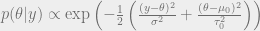
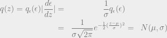
This is a very elementary example, and completely lifted from BDA. Consider data , parameterized by the model , with a gaussian likelihood.

We also use a gaussian prior

Now, to get the posterior, we use Bayes, but as we are ‘given’ the data, we treat as constant, so it basically becomes the product of the prior times likelihood, with an unknown normalizing constant .

Now when we plug our individual formulas into this, we get a product of two gaussians, which is also a gaussian.

After going through the exercise of completing the square (and treating terms not containing as constant, etc), we get

where and

We can interpret this result as a compromise between the prior and the ‘data’ term as connoted by – in the first version below, we ‘adjust’ the estimate given by the prior to account for the data.

Equivalently, we can say that the data has ‘shrunk’ towards the prior mean:

It’s a bit more interesting when we have more than one data point. What happens when we have lots of lots of data, as we would in say, a general deep learning setting?

We use the same ideas, with iid assumptions and come up with a similar formulation, summarized by a sample mean:

This can be summarized with the sample mean – sufficient statistics – .

where

and

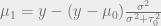
Now, after all this, we get to the crux or nub. Initially, when there is no data, we rely entirely on the prior belief. As data starts to arrive, the prior (embodied by ) gets slowly weighted out by the data term. When we have a large number of data points , our uncertainty term vanishes:

Here, we converge to an estimate parameterized by the sample mean, and the variance parameter goes to zero. In other words, as we get more and more points, we are able to make a more accurate prediction of the mean. In a perverse way, this struck me as one reason why we resort to maximum likelihood in deep learning problems. As the amount of data increases, the uncertainty in estimating the model decreases, with the parameter eventually converging to a point estimate.

BDA3, Chapter 2: https://avehtari.github.io/BDA_course_Aalto/

In this note, we take a look at the reparameterization trick, an idea that forms the basis of the Variational Autoencoder. My material here comes from the fantastic paper by Ruiz et al [1]. The main idea is that the reparameterization trick [4,5] gives us a lower variance estimator than that obtained from the score function gradient, but suffers because the class of distributions to which it can be applied is somewhat limited – Kingma and Welling discusses Bernaulli and Gaussian variants. Nevertheless, it is possible to remedy this defect, as is done in papers [1], [2], [3]. The paper by Ruiz is especially instructive. It walks us through the machinery involved in reparameterization and discusses variance reduction [Casella and Berger, Robert and Casella] for variational inference – also [BBVI]. I was originally intending on writing a much more complete summary of the papers [1], [2], [3] but ran out of juice, leaving it for the future as might transpire (or not). If I may insert inappropriately (also, perhaps to acknowledge a decade that just ended):

What might have been is an abstraction
Remaining a perpetual possibility
Only in a world of speculation.
What might have been and what has been
Point to one end, which is always present.

Notwithstanding such tangential musings, it behooves us to study [Casella and Berger]. The authors note that it is a 22 month long course to learn statistics the hard way. Incidentally, the style of books bearing George Casella’s imprint – either actual or inspirational – ([Robert and Casella], [Robert]) very much reminds me of [Bender and Orszag], with engaging quotes from Holmes and their straight forward slant on equations.

Recall that in variational problems we are interested in obtaining the ELBO. We briefly derive this using Jensen’s inequality ()

Take the joint form presented in Ruiz:

Or

Or

The equation written in this form is quite instructive. We want to optimize the joint by varying the variational parameters v through the surrogate distribution .

Our aim is to obtain Monte Carlo estimates of the gradient (by taking expectations), but this is not possible as is. However, it is possible to arrange this as follows:

This is known as the score function estimator, or the REINFORCE gradient. We can view it as a discrete gradient that allows us to take gradients of non-differentiable functions by taking samples.

However, the estimate obtained tends to be noisy, and needs provisos for variance reduction – e.g. Rao-Black Wellization, control variates.

A principal contribution of the VAE approach is that we have an alternative way to derive the estimator, one that is generally of lower variance than the score function method described above. That being said, it has the drawback that the method is not as widely applicable as the score function approach.

Recall that we would like to take gradients of the term containing the log joint in the ELBO.

In this equation, we can take samples , but as the estimator contains variational parameters within it, we cannot carry out any sort of diffentiation operations to it with respect to – necessary to take gradients. The reparameterization trick gets around this problem.

We derive an alternative estimator by transforming to a distribution that does not depend on so that we can now take the gradient operator inside the expectation. For this to work, we rely on what they call a ‘standardization’ operation to transform into another distribution independent of (and other terms containing ). In the end, we want to have something like this:

We have pushed the gradient operator inside the expectation which allows us to take samples and allow taking gradients from it.

That’s a lot of words. Let us derive this estimator to put it more concretely.

We assume that there exists an invertable transformation with pdfs . In some cases, it is possible to find a transformation such that the reparameterized distribution is independent of the variational parameters . For example, consider the standard normal distribution:

We can consider this as the standardized version of a normal distribution .

Transform (pretend 1D for now):

For more general cases, the differential is replaced by a Jacobian:

After standardization, we lose dependence on : so that

Now we can take gradient and move it inside the expectation:

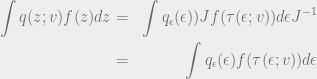
The standardization procedure is now extended so that is weakly dependent on – it has zero mean, but it’s first moment does not depend on . Nevertheless, has dependence on the variational parameters. In this case, the expectation will have to be evaluated term by term with chain rule

As we can see, the first term is the regular reparameterization gradient. The second term is the score function estimator, a correction term for this version of this standardization setup.

In the case of the normal distribution, the second term vanishes.

The terms are massaged so as to look like control variates, an idea used in Monte Carlo variance reduction. The authors note that while Rao-Blackwellization is not used in the paper, it is perfectly reasonable to use the setup in conjuction with it, as is done in Black Box Variational Inference [BBVI], where both Rao-Blackwellization and control variates are used to reduce the variance of the estimator.

The basic idea of control variates is as follows ([Casella and Berger] – Chapter 7 on “Point Estimation”). Given an estimator satisfying , we seek to find another estimator of lower variance, using an estimator with :

The variance for this estimator is (Casella and Berger):

We would get lower variance for than if we could find such that .

To get back to our variational estimator, rewrite as follows for it to be interpretable as control variates (see [1]):

In the first line, we have the score function expression, which is modified in subsequent lines. It is not entirely clear to me how the expectation of the terms that correct the noisy gradient is zero, but I suppose we will take it in the spirit with which it was intended.

[1] Ruiz et al: The generalized reparameterization gradient: https://arxiv.org/abs/1610.02287

[2] Naesseth et al: Reparameterization Gradients through Acceptance-Rejection Sampling Algorithms: https://arxiv.org/abs/1610.05683

[3] Figurnov et al: Implicit Reparameterization Gradients: https://arxiv.org/abs/1805.08498

[4] Kingma and Welling: Autoencoding Variational Bayes: https://arxiv.org/abs/1312.6114

[5] Rezende, Mohamed and Wierstra: Stochastic Backpropagation and Approximate Inference in Deep Generative Models: https://arxiv.org/abs/1401.4082

[BBVI] Black Box Variational Inference: https://arxiv.org/abs/1401.0118

[Casella and Berger]: Statistical Inference: https://www.amazon.com/Statistical-Inference-George-Casella/dp/0534243126

[Robert and Casella]: Monte Carlo Statistical Methods: https://www.amazon.com/Monte-Statistical-Methods-Springer-Statistics/dp/1441919392

[Robert]: The Bayesian Choice: https://www.amazon.com/Bayesian-Choice-Decision-Theoretic-Computational-Implementation/dp/0387715983

[Bender and Orszag]: Advanced Mathematical Methods for Scientists and Engineers: https://www.amazon.com/Advanced-Mathematical-Methods-Scientists-Engineers/dp/0387989315

I wanted to write about normalizing flows, but instead I am putting up something a bit more fundamental, as it forms a building block in the normalizing flows scheme (and even in deriving the reparameterization trick [8,9]), and one which had caused some mild discomfort when I had first looked that body of work (Variational Normalizing Flows [1], Inverse Autoregressive Flow [2], NICE [3], RealNVP [4], Glow [5], Masked Autoregressive Flow [6] (a must read) and this comprehensive review by Deepmind authors [7]).

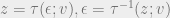
The question to be asked is this: given a pdf , and a transformation , how do we calculate the pdf of the variable ?

Intuitively, we can call it conservation of probability mass:

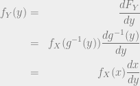
or (use modulus to keep sign positive)

Below, we go over the machinery in Casella and Berger [0].

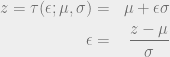
Consider the pdf of a continuous random variable : , with the transformation from : . Then the CDF of is given by:

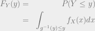
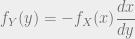
Here, we should make note of whether the transformation is an increasing or decreasing function. In the case of it being an increasing function, the expression becomes:

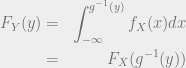
assuming that is supported in . Likewise, if is a decreasing function, we take the limits from to . This is because for any , in this case. This is made use of in the formula for .

Typically (again, from Casella and Berger), we sum up the contributions in piecewise fashion where the functions are increasing/decreasing.

By definition, the pdf is obtained by differentiating the cdf. As before, we treat the case for the function being increasing or decreasing separately.

When is an increasing function

The case where is a decreasing function gets a negative sign.

We can combine both of these into a single formula

In Casella and Berger, the multivariate form is discussed in the chapter “Multiple Random Variables”, with some additional constraints that the function must be one-one and onto. We can see why these constraints arise: In the univariate case above needs to exist, so the function must be one-one (i.e. have only one equivalent mapping in the inverse), and onto (no point must be left out).

Assuming that for a continuous random vector , we have a transformation (with sloppy notation) , functions that are one-one and onto, we should have an inverse transformation .

The transformed distributions are related analogously to the univariate case, with the derivative now being replaced by a Jacobian, whose absolute value we use.

where

The above formalism forms the general idea behind flow based generative models. We start with some distribution (which could be, say, a gaussian), and then transform it into more and more expressive distributions. We do the bookkeeping by means of the transformation machinery described above.

Variational Normalizing Flows [1]

0. Casella and Berger: https://www.amazon.com/Statistical-Inference-George-Casella/dp/0534243126
1. Variational Normalizing Flows: https://arxiv.org/abs/1505.05770
2. Inverse Autoregressive Flow: https://arxiv.org/abs/1606.04934
3. NICE: https://arxiv.org/abs/1410.8516
4. RealNVP: https://arxiv.org/abs/1605.08803
5. Glow: https://arxiv.org/abs/1807.03039
6. Masked Autoregressive Flow: https://arxiv.org/abs/1705.07057
7. Review by Deepmind authors: https://arxiv.org/abs/1912.02762
8. Kingma and Welling: https://arxiv.org/abs/1312.6114
9. Rezende, Mohamed and Wierstra: https://arxiv.org/abs/1401.4082

In this note, we explain through an argument and a bit of hand waving, why gradient clipping makes sense in the Wasserstein GAN [1].

We briefly examine the main ideas behind the WGAN work for context.

We would like to produce samples from a generator , which we would like to come from the same distribution as the ground truth . This is achieved by minimizing the Wasserstein distance between and . We can propose this problem in primal space through Optimal Transport.

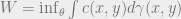
where , ; i.e. we sample and send it through the generator, or in other words, we push forward to : ; and . The Wasserstein distance is characterized by a particular type of joint distribution of and , in that we must look for candidates whose marginals reduce to – ; .

The form for the distance measure can be specified as a Euclidean distance, in which case we term this quantity a Wasserstein distance:

The Wasserstein distance will have a root:

Generally in the literature, we find use of . The original Monge problem was with , . When we use the squared distance with , we come across something called “Brenier’s theorem” in the Monge problem.

In the current setting, is used, as it becomes expedient to set up the discriminator form this way. In principle, we can directly optimize the Wasserstein distance itself through Sinkhorn divergences (see [3]). However, it is as such not so simple (expensive?) to optimize the Wasserstein distance, so the WGAN paper used an ingenious trick, of transforming the problem to its dual equivalent through the Kantorovich-Rubinstein inequality. This is possible only when we use . I hope to put up a proof of the Kantorovich-Rubinstein inequality in the not so distant future.

After transforming the problem to its dual form with the Kantorovich-Rubinstein inequality, we get the following expression for the discriminator objective:

Expanding that a bit, we would like to get the discriminator (parameterized by ) that maximizes the above. The constraint, of course is that these functions should be 1-Lipshitz continuous.

As we can see, the form is amenable to gradient descent:

Next, we talk about how the Lipshitz constraint is imposed, which, if we are to remind ourselves, is the raison d’etre for this note.

Let us first sketch out the Lipshitz formula in black and white.

Given a real valued function , a function is Lipshitz continuous [4] if there exists a constant such that

The Kantorovich-Rubinstein inequality demands that we have . The question then arises as to how we can enforce this constraint. The paper’s recipe is to ‘clip’ the weights so that they lie in a ball ( being the dimensionality). Here, we try to intuit why this might work through some simple analysis.

Consider a discriminator with a single layer, carrying out the operation:

We can do away with the non-linearity for now (well, ReLU will zero things out, so we can be sure that it won’t increase the norm). Then when we take norms,

For it to satisfy the 1-Lipshitz constraint we need . One way of enforcing this is to arbitrarily clip the weights to some small value. They use . The authors note that this is a ‘clearly terrible’ way of enforcing the condition because it reduces capacity, and could also lead to vanishing gradients.

In the follow up work [3], the authors implement the constraint in a more principled way by means of an additional penalty term that asks that the gradient norm be less than unity. This appeals to the idea that the lipshitz equation is like a slope, and when we take two points , that are very close to each other, we get the gradient.

1. Wasserstein GAN: https://arxiv.org/abs/1701.07875
2. Improved training of Wasserstein GANs: https://arxiv.org/pdf/1704.00028.pdf
3. Learning generative models with Sinkhorn divergences: https://arxiv.org/abs/1706.00292
4. Lipshitz conitnuity: https://en.wikipedia.org/wiki/Lipschitz_continuity

It has been more than 2 1/2 years since the WGAN paper came out. This was a landmark effort that brought to light connections between optimal transport and GANs. It is also a formidable paper to come to terms with (I would not have felt up to reviewing that paper, not without understanding the duality proofs). And of course, the work is a shining example of a method that can be used in practice in applications. I have never felt up to putting up a review for this paper – so far – because there are some components there that I haven’t been able to prove. And when you put up results that you don’t fully have a feel for, it feels a bit disingenuous. The story is akin to the analogous situation in Chess where lets say, you are asked to evaluate a position with a bishop, knight and king against king, which you know is a win, but cannot do it over the board. I have also had some realizations along the way. Chief among them is that we cannot be self-respecting practitioners without studying convex optimization. This is probably as important as probability theory is, perhaps even more so. The second realization was more of a prosaic affirmation, that we ought to do some – useless – pen and paper work to keep our sanity. When there are so many things we have no control over (e.g. the capriciousness of the attention curve), it is reassuring that there are things that go beyond getting things to work, build and engineer. You can take all the time you want to, but in the end, there is truth, and that allows us to let go of the stress that our chaotic world produces.

Thanks to the WGAN paper, and the somewhat unrelated follow up on Wasserstein Autoencoders – which is eminently much more readable – I have been digging up Optimal Transport literature for instruction and entertainment. Maybe application also some day.

Having dispensed with the pourparlers, we can now get on with the matter of the moment (I hope the old sweats had found something else to do when they looked away). This time, I would like to provide a proof of the Kantorovich duality from an unexpectedly accessible tutorial on OT. It is to be noted that this is NOT the Kantorovich-Rubinstein duality used in the WGAN work. That emerges as a consequence of the Kantorovich duality, and is treated separately. My material comes from the excellent tutorial [1].

For the record, what bothered me in the WGAN paper most was the Kantorovich-Rubinstein duality which is a critical step in the paper’s presentation. In order to do justice to the paper, it is necessary for us to understand duality proofs. The Kantorovich-Rubinstein inequality arises as a consequence of the main duality proof, which the current article makes an attempt at explaining for the discrete problem.

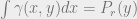
Before we set up the discrete problem from [1], it helps to introduce ourselves with the main ideas. The optimal transport problem can be seen as a transporting mass between a source and target domain, characterized by a joint function , the transport plan. The joint has the property that when we take its marginals, we get the source and target masses.

We would like to take the minimum cost computed from all the s available, giving us an optimal metric. The quantity is the distance. When we take the Euclidean distance , we call this a Wasserstein distance. The original problem by Monge concerned itself with moving mounds of earth between points, with . The problem was defined such that one wanted to transport earth from a point to another point using a mass conservation condition. Apparently, this formulation posed several problems, such as non-existence (as mass cannot be split).

The above equation is written for the continuous problem. In the discrete setting, we replace the integral by a sum, so that what results is a dot product . We work in the discrete setting to stay compatible with the notes in [1].

Let us consider the problem where we have point masses , and point masses , and we would like to transport to with minimum cost. The transportation plan in this case is the ‘joint’ , and the cost is where , with , .

The problem becomes:

Here, it is worth our while look at the dimensions of the quantities. is of dimension ; is of dimension ( flattened into a vector), so the quantity should be of dimension . Likewise, should be of dimension . We are now ready to set up the objective.

With our primal discrete OT problem having been formulated, we first add a few terms to it, carefully making sure that it does not alter the expression by suitably adding infs and sups. We recast the original problem (the primal) into an optimization problem over .

We take the supremum of this expression over . When the constraints are satisfied, it equals the desired expression . Otherwise, its maximum would be . In fact, we can adjust the values of so that the expression becomes arbitrarily large.

We have made no changes to the original problem, except for adding a few extra layers of logic that turn the problem into finding an optimizer over .

I should note that this logic had eluded comprehension until I had chanced upon the tutorial [1], when something moved from under the brown fog of the brain. In some ways, one either gets it or one doesn’t. If one doesn’t, then it grates the soul, like a taxi throbbing waiting, while it fixes us with the aforesaid logic, leaving us sprawling on a pin, pinned and wriggling against the wall. And then, it emerges, announcing its arrival to say:

“I am Lazarus, come from the dead
Come back to tell you all
I shall tell you all …”

After setting up the indicator variables, we now add another piece. Take the infimum on both sides. When we do this, the branch with vanishes, as we can find a lower value for the expression, which in this case has to be the one that satisfies the constraint.

It can be seen that the resulting expression is the equation for the primal. Observe also that the way the constraint gets manipulated is rather reminescent of the Lagrange multiplier machinery for constrained optimization (Boyd and Vandenberghe).

In the next few manipulations, we arrive at the expression for the dual. This time, we appeal to another trick of swapping the inf and the sup.

The four lines constituting the manipulation are explained below. In the first (equation (3)), we restate the expression as before. In the second, we swap inf and sup. This step is called the minimax principle, wisdom that I will take for granted (I contradict what I said earlier, about not putting up things that I don’t understand, but we will look the other way for now). The third equation is a rearrangement, fairly uncomplicated. The last step (equation (6)) needs a bit of explanation. In this, we again reinterpret the problem as one of constrained optimization, as we do with Lagrange multipliers. The constraint is to be viewed in a component wise sense.

And there we have it. We have just derived the duality equations subject to the cost constraint.

In fact, it seems that we have equality between the primal and dual problems (is that correct?).

1. Notions of optimal transport theory and how to implement them on a computer
: https://arxiv.org/abs/1710.02634

2. Computational Optimal Transport (Peyre and Cuturi): https://arxiv.org/abs/1803.00567

3. WGAN: https://arxiv.org/abs/1701.07875

4. WAE: https://arxiv.org/abs/1711.01558

5. Convex Optimization (Boyd and Vandenberghe): https://web.stanford.edu/~boyd/cvxbook/

In Tacotron, it is recommended that we generate several output tokens at each decoder timestep, and then use one (or all, or some combination thereof) of them as input for the next timestep. While coding this up, I inadvertently created a bug for myself which went undetected for a long long time. To set things up in black and white, we create an example that shows how we should (and should not) reshape pytorch tensors in these scenarios.

Assume that we have a vector of size 8 in batches of 5 elements (5,8). In the end, we would like to produce 2 batches of 5, with vectors of size 4 – we break off the size 8 vector into two (2,5,4). The reason we do this is that our desired decoder output per timestep is of size 4, but since we produce a vector of size 8 by agglomerating two frames/timesteps into one, we would need to break it to read off the individual vectors.

Now, we would like to reshape this vector to produce 2 batches of frames of size 4. So the first four columns go into the first bucket, while the rest goes into the other bucket.

The point behind shaping it as (2,5,4) is that we can read them off as x[0] and x[1] which comprise our desired output for timesteps t+0, t+1, with the total number of decoder timesteps being (we would actually stop when the EOS token is produced, but disregard that for now) 2T.

The above is all obvious when we look at it retrospectively (and I, like Tiresius, perceived the bug and foretold the rest), but in my code, I had it as follows:

So, now we are traversing each row to grab 4 elements as we go along, and then dropping them in the same bucket until we do this 5 times, after which we drop the remainder in the other bucket. The correct way to do it would be to drop them off alternately in different buckets.

Needless to say, the choir will sneer for being preached upon. Nevertheless, it is fair to say that we mustn’t just make the shapes fit while reshaping. The ordering also matters, and its not a bad thing to be mindful of that to save us some heartaches and unnatural shocks that code is heir to.

A good paper comes with a good name, giving it the mnemonic that makes it indexable by Natural Intelligence (NI), with exactly zero recall overhead, and none of that tedious mucking about with obfuscated lookup tables pasted in the references section. I wonder if the poor (we assume mostly competent) reviewer will even bother to check the accuracy of these references (as long as we don’t get any latex lacunae ??) in their already overburdened roles of parsing difficult to parse papers, understanding their essence and then their minutiae, and on top of that providing meaningful feedback to the authors.

Tacotron is an engine for Text To Speech (TTS) designed as a supercharged seq2seq model with several fittings put in place to make it work. The curious sounding name originates – as mentioned in the paper – from obtaining a majority vote in the contest between Tacos and Sushis, with the greater number of its esteemed authors evincing their preference for the former. In this post, I want to describe what I understand about these architectures designed to produce speech from text, and the broader goal of disentangling stylistic factors such as prosody and speaker identity with the aim of combining them in suitable ways.

Tacotron is a seq2seq model taking in text as input and dumping speech as output. As we all know, seq2seq models are used ubiquitously in machine translation and speech recognition tasks. But over the last two or three years, these models have become usable in speech synthesis as well, largely owing to the Tacotron (Google) and DeepVoice (Baidu) works. In TTS, we take in characters or phonemes as input, and dump out as a speech representation. At the time of publication (early 2017), this model was unique in that it demonstrated a nearly end to end architecture that could produce plausible sounding speech. Related in philosophy was the work by Baidu (DeepVoice 1 – I think) which also had a seq2seq TTS setup, but which was not really end to end because it needed to convert text (grapheme) to phoneme and then pass that in to subsequent stages. The DeepVoice architecture has also evolved with time, and has produced complex TTS setups adapted for tasks such as speaker adaptation and creating speaker embeddings in transfer learning contexts with few data. Nevertheless, we should note that speech synthesis is probably never going to be end to end (as the title of the paper says) owing to the complexity of the pipeline. In Tacotron, we generate speech representations which need to be converted to audio in subsequent steps. This makes speech a somewhat difficult problem to approach – speaking personally – for the newbie unlike images where we can readily see the output. Even so, we can make do by looking at spectrograms. The other problem in speech is the lack of availability of good data. It costs a lot of money to hire a professional speaker!

Architecture

At a high level, we could envisage Tacotron as an encoder-decoder setup where text embeddings get summarized into a context by the encoder, which is then used to generate output speech frames by the decoder. Attention modeling is absolutely vital in this setup for it to generalize to unseen inputs. Unlike NMT or ASR, the output is inflated, so that we have many output frames for an input frame. Text is a highly compressed representation whereas speech (depending on the representation) is highly uncompressed.

Several improvements are made to bolster the attention encoder-decoder model, which we describe below.

1. Prenet: This is a bottleneck layer of sorts consisting of full connections. Importantly, it uses dropout which serves as a regularization mechanism for it to generalize to test samples. The paper mentions that scheduled sampling does not work well for them. Prenet is also used in the decoder.
2. CBHG: “Convolutions, FilterBanks and Highway layers, Gated Recurrent Units”. We could view the CBH parts as preprocessing layers taking 1-3-5-… convolutions (Conv1d) and stacking all of them up after maxpooling them. It makes note of relationships between words of varying lengths (n-grams) and collates them together. This way, we agglomerate the input characters to a more meaningful feature representation taking into account the context at the word level. These are then sent to a stack of highway layers – a play on the residual networks idea – before being handed off to the recurrent encoder. I’ve described the architecture in more detail in another post. The “G” in CBHG is the recurrent encoder, specified as a stack of bidirectional Gated Recurrent Units.
3. Reduction in output timesteps: Since we produce several similar looking speech frames, the attention mechanism won’t really move from frame to frame. To alleviate this problem, the decoder is made to swallow inputs only every ‘r’ frames, while we dump r frames as output. For example, if r=2, then we dump 2 frames as output, but we only feed in the last frame as input to the decoder. Since we reduce the number of timesteps, the recurrent model should have an easier time with this approach. The authors note that this also helps the model in learning attention.

Apart from the above tricks, the components are setup the usual way. The workflow for data is as follows.

We pass the processed character inputs to the prenet and CBHG, producing encoder hidden units. These hidden units contain linguistic information, replacing the linguistic context used in older approaches (Statistical Parametric Speech Synthesis or SPSS). Since this is the ‘text’ summary, we can also think of it as seed for other tasks such as in the Tacotron GST works (Global Style Tokens) where voices of different prosodic styles are summarized into tokens which can then be ‘mixed’ with the text summaries generated above.

On the decoder side, we first compute attention in the so-called attention RNN. This term caused me a lot of confusion initially. The ‘attention RNN’ is essentially the block where the we compute the attention context, which is then concatenated with the input (also ejected by a prenet) and then sent to a recurrent unit. The input here is a mel spectrogram frame. The output of the attention RNN is then sent to a stack of recurrent units and projected back to the mel dimensions. Also, this stack uses residual connections.

Finally, instead of generating a single mel frame for each decoder step, we produce ‘r’ output frames, the last of which gets used as input for the next decoder step. This is termed the ‘reduction factor’ in the paper, with the number of decoder timesteps getting reduced by a factor or ‘r’. As we are producing a highly uncompressed speech output, it makes sense to assist the RNNs by reducing their workload. It is also said to be critical in helping the model learn attention.

Generalization comes from dropout in this case, with ground truth being fed – teacher forced – during training as input decoder frames. Contrast this with running in inference mode where one has to use decoder generated outputs as input for the next timestep. In scheduled sampling, the amount of teacher forcing is tapered down as the model trains. Initially, a large amount of ground truth is used, but as the models learns with time, we slowly taper off to inference mode with some sort of schedule. The other way is to use GANs to make the inference mode (fake) behave like teacher forced output (real) with a discriminator being used to tell them apart; the idea being that the adversarial game results in the generator producing inference mode samples that are indistinguishable from the desired, teacher forced mode output. This approach is named “Professor Forcing”.

Postprocessing network

Mel spectrogram frames generated by the network are converted back to audio with the postprocessing scheme. This postprocessing scheme is described in the literature as a ‘vocoder’ or backend. In the original tacotron work, the process involves first converting the mel frames into linear spectrogram frames with a neural network to learn the mapping. We actually lose information going from linear to mel spectrogram frames. The mapping is learnt using a CBHG network (not necessarily encoder-decoder as the input and output sequences have the same lengths) as used in the front end part of the setup computing linguistic context. In the end, audio is produced by carrying out an iterative procedure called Griffin-Lim on the linear spectrogram frames. In more recent works, the backend part is replaced by a Wavenet for better quality samples.

Refinements in Tacotron 2

Tacotron 2’s setup is much like its predecessor, but is somewhat simplified, in in that it uses convolutions instead of CBHG, and does away with the (attention RNN + decoder layer stack) and instead uses two 1024 unit decoder layers. In addition to this, it also has provisions to predict the probability of emission of the ‘STOP’ token, since the original Tacotron had problems predicting the end of sequence token and tended to get stuck. Also, Tacotron 2 discards the reduction factor, but adds location sensitive attention as in Chorowski et al’s ASR work to help the attention move forward. Supposedly, these changes obviate the need for the r-trick. In addition to location sensitive attention, the GST Tacotron works also use Alex Graves’ GMM attention from the handwriting synthesis works.

There are many other minutiae as well such as using MSE loss instead of L1,  which I suppose would qualify as tricks to be noted if one is actually creating these architectures.

Controlling speech with style tokens

The original Tacotron work was designed for a single speaker. While this is an important task in and of itself, one would also like to control various factors associated with speech. For example, can we produce speech from text for different speakers, and can we modify prosody? Unlike images where these sorts of unsupervised learning problems have been shown to be amenable to solutions (UNIT, CycleGAN, etc.), in speech we are very much in the wild west, and the gold rush is on. Built on top of Tacotron, Google researchers have made attempts at exercising finer control over factors by creating embeddings for prosodic style and speakers (also in Baidu’s works), which they call Global Style Tokens (GST).

Style Tokens are vectors exemplifying prosodic style which are shared across examples and learnt during training. They are randomly initialized, and compared against a ‘reference’ encoding (which is just a training audio example ingested by the reference encoder module) by means of attention, so that our audio example is now a weighted sum of all the style tokens. During inference, we can manually adjust the weights of each style token, or simply supply a reference encoding (again, spat out by the style encoder after putting in reference audio).

References

1. UNIT: Unsupervised Image to Image Translation Networks: https://arxiv.org/abs/1703.00848

2. CycleGAN: https://arxiv.org/abs/1703.10593

3. Tacotron: Towards End to End Speech Synthesis: https://arxiv.org/abs/1703.10135

4. Tacotron-2: Natural TTS Synthesis by Concatenating Wavenet on Mel Spectrogram Predictions: https://arxiv.org/abs/1712.05884

5. Towards End-to-End Prosody Transfer for Expressive Speech Synthesis with Tacotron: https://arxiv.org/abs/1803.09047

6. (GST) Style Tokens: Unsupervised Style Modeling, Control and Transfer in End-to-End Speech Synthesis: https://arxiv.org/abs/1803.09017

7. Alex Barron’s notes (excellent) describing Tacotron, implementation and woes: http://web.stanford.edu/class/cs224s/reports/Alex_Barron.pdf

8. Baidu Deep Voice 3: http://research.baidu.com/Blog/index-view?id=91

9. (Speaker adaptation with Deep Voice) Neural Voice Cloning with a few samples: https://arxiv.org/abs/1802.06006

10. Professor Forcing: https://arxiv.org/abs/1610.090381

11. Alex Graves: “Generating Sequences With Recurrent Neural Networks”: https://arxiv.org/abs/1308.0850

12. CBHG: Fully Character-Level Neural Machine Translation Without Explicit Segmentation: https://arxiv.org/abs/1610.03017