K3XEC

Interested in future updates? Follow me on mastodon at @paul@soylent.green. Posts about hz.tools will be tagged #hztools.

🐶 Want to jump right to the draft? I'll be maintaining ARF going forward at /draft-tagliamonte-arf-00.txt.

It’s true – processing data from software defined radios can be a bit complex 👈😏👈 – which tends to keep all but the most grizzled experts and bravest souls from playing with it. While I wouldn’t describe myself as either, I will say that I’ve stuck with it for longer than most would have expected of me. One of the biggest takeaways I have from my adventures with software defined radio is that there’s a lot of cool crossover opportunity between RF and nearly every other field of engineering.

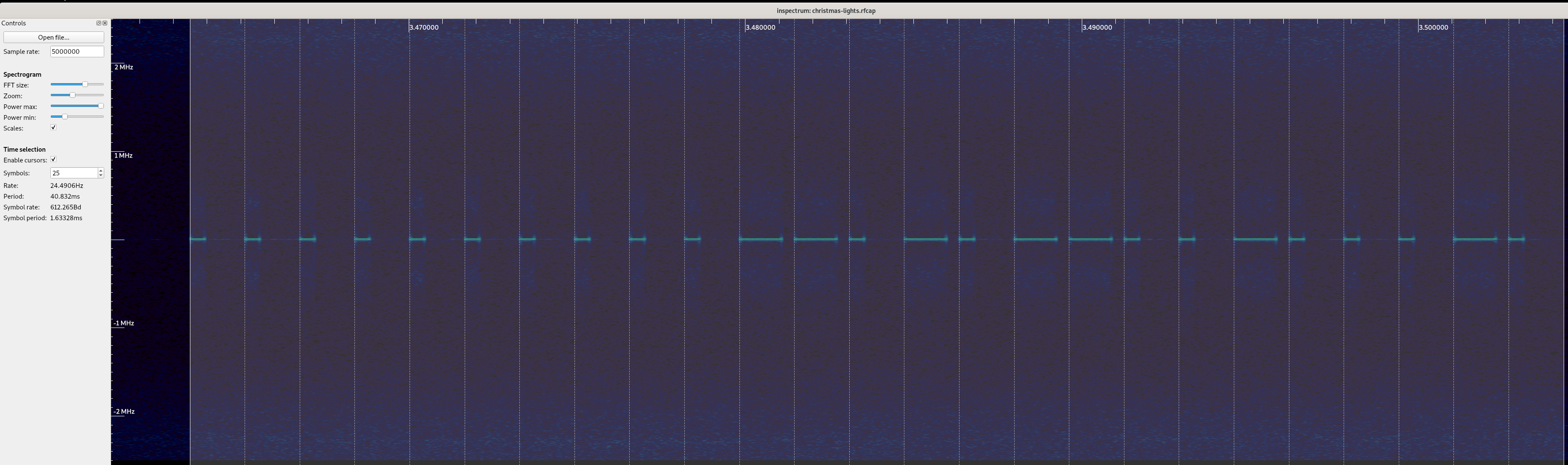
Fairly early on, I decided on a very light metadata scheme to track SDR captures, called rfcap. rfcap has withstood my test of time, and I can go back to even my earliest captures and still make sense of what they are – IQ format, capture frequencies, sample rates, etc. A huge part of this was the simplicity of the scheme (fixed-lengh header, byte-aligned to supported capture formats), which made it roughly as easy to work with as a raw file of IQ samples.

However, rfcap has a number of downsides. It’s only a single, fixed-length header. If the frequency of operation changed during the capture, that change is not represented in the capture information. It’s not possible to easily represent mulit-channel coherent IQ streams, and additional metadata is condemned to adjacent text files.

ARF (Archive of RF)

A few years ago, I needed to finally solve some of these shortcomings and tried to see if a new format would stick. I sat down and wrote out my design goals before I started figuring out what it looked like.

First, whatever I come up with must be capable of being streamed and processed while being streamed. This includes streaming across the network or merely written to disk as it’s being created. No post-processing required. This is mostly an artifact of how I’ve built all my tools and how I intereact with my SDRs. I use them extensively over the network (both locally, as well as remotely by friends across my wider lan). This decision sometimes even prompts me to do some crazy things from time to time.

I need actual, real support for multiple IQ channels from my multi-channel SDRs (Ettus, Kerberos/Kracken SDR, etc) for playing with things like beamforming. My new format must be capable of storing multiple streams in a single capture file, rather than a pile of files in a directory (and hope they’re aligned).

Finally, metadata must be capable of being stored in-band. The initial set of metadata I needed to formalize in-stream were Frequency Changes and Discontinuities. Since then, ARF has grown a few more.

After getting all that down, I opted to start at what I thought the simplest container would look like, TLV (tag-length-value) encoded packets. This is a fairly well trodden path, and used by a bunch of existing protocols we all know and love. Each ARF file (or stream) was a set of encoded “packets” (sometimes called data units in other specs). This means that unknown packet types may be skipped (since the length is included) and additional data can be added after the existing fields without breaking existing decoders.

tag flags length value Heads up! Once this is posted, I'm not super likely to update this page. Once this goes out, the latest stable copy of the ARF spec is maintained at draft-tagliamonte-arf-00.txt. This page may quickly become out of date, so if you're actually interested in implementing this, I've put a lot of effort into making the draft comprehensive, and I plan to maintain it as I edit the format.

Unlike a “traditional” TLV structure, I opted to add “flags” to the top-level packet. This gives me a bit of wiggle room down the line, and gives me a feature that I like from ASN.1 – a “critical” bit. The critical bit indicates that the packet must be understood fully by implementers, which allows future backward incompatible changes by marking a new packet type as critical. This would only really be done if something meaningfully changed the interpretation of the backwards compatible data to follow.

Flag Description 0x01Critical (tag must be understood)

Within each Packet is a tag field. This tag indicates how the contents of the value field should be interpreted.

Tag ID Description 0x01Header 0x02Stream Header 0x03Samples 0x04Frequency Change 0x05Timing 0x06Discontinuity 0x07Location 0xFEVendor Extension

In order to help with checking the basic parsing and encoding of this format, the following is an example packet which should parse without error.

 00, // tag (0; no subpacket is 0 yet)
 00, // flags (0; no flags)
 00, 00 // length (0; no data)
 // data would go here, but there is none

Additionally, throughout the rest of the subpackets, there are a few unique and shared datatypes. I document them all more clearly in the draft, but to quickly run through them here too:

UUID

This field represents a globally unique idenfifer, as defined by RFC 9562, as 16 raw bytes.

Frequency

Data encoded in a Frequency field is stored as microhz (1 Hz is stored as 1000000, 2 Hz is stored as 2000000) as an unsigned 64 bit integer. This has a minimum value of 0 Hz, and a maximum value of 18446744073709551615 uHz, or just above 18.4 THz. This is a bit of a tradeoff, but it’s a set of issues that I would gladly contend with rather than deal with the related issues with storing frequency data as a floating point value downstream. Not a huge factor, but as an aside, this is also how my current generation SDR processing code (sparky) stores Frequency data internally, which makes conversion between the two natural.

IQ samples

ARF supports IQ samples in a number of different formats. Part of the idea here is I want it to be easy for capturing programs to encode ARF for a specific radio without mandating a single iq format representation. For IQ types with a scalar value which takes more than a single byte, this is always paired with a Byte Order field, to indicate if the IQ scalar values are little or big endian.

ID Name Description 0x01f32interleaved 32 bit floating point scalar values 0x02i8 interleaved 8 bit signed integer scalar values 0x03i16interleaved 16 bit signed integer scalar values 0x04u8 interleaved 8 bit unsigned integer scalar values 0x05f64interleaved 64 bit floating point scalar values 0x06f16interleaved 16 bit floating point scalar values Header

Each ARF file must start with a specific Header packet. The header contains information about the ARF stream writ large to follow. Header packets are always marked as “critical”.

magic flags start guid site guid #st

In order to help with checking the basic parsing and encoding of this format, the following is an example header subpacket (when encoded or decoded this will be found inside an ARF packet as described above) which should parse without error, with known values.

00, 00, 00, fa, de, dc, ab, 1e, // magic
00, 00, 00, 00, 00, 00, 00, 00, // flags
18, 27, a6, c0, b5, 3b, 06, 07, // start time (1740543127)

// guid (fb47f2f0-957f-4545-94b3-75bc4018dd4b)
fb, 47, f2, f0, 95, 7f, 45, 45,
94, b3, 75, bc, 40, 18, dd, 4b,

// site_id (ba07c5ce-352b-4b20-a8ac-782628e805ca)
ba, 07, c5, ce, 35, 2b, 4b, 20,
a8, ac, 78, 26, 28, e8, 05, ca

Stream Header

Immediately after the arf Header, some number of Stream Headers follow. There must be exactly the same number of Stream Header packets as are indicated by the num streams field of the Header. This has the nice effect of enabling clients to read all the stream headers without requiring buffering of “unread” packets from the stream.

id flags fmt bo rate freq guid site

In order to help with checking the basic parsing and encoding of this format, the following is an example stream header subpacket (when encoded or decoded this will be found inside an ARF packet as described above) which should parse without error, with known values.

00, 01, // id (1)
00, 00, 00, 00, 00, 00, 00, 00, // flags
01, // format (float32)
01, // byte order (Little Endian)
00, 00, 01, d1, a9, 4a, 20, 00, // rate (2 MHz)
00, 00, 5a, f3, 10, 7a, 40, 00, // frequency (100 MHz)

// guid (7b98019d-694e-417a-8f18-167e2052be4d)
7b, 98, 01, 9d, 69, 4e, 41, 7a,
8f, 18, 16, 7e, 20, 52, be, 4d,

// site_id (98c98dc7-c3c6-47fe-bc05-05fb37b2e0db)
98, c9, 8d, c7, c3, c6, 47, fe,
bc, 05, 05, fb, 37, b2, e0, db,

Samples

Block of IQ samples in the format indicated by this stream’s format and byte_order field sent in the related Stream Header.

id iq samples

In order to help with checking the basic parsing and encoding of this format, the following is an samples subpacket (when encoded or decoded this will be found inside an ARF packet as described above). The IQ values here are notional (and are either 2 8 bit samples, or 1 16 bit sample, depending on what the related Stream Header was).

01, // id
ab, cd, ab, cd, // iq samples

Frequency Change

The center frequency of the IQ stream has changed since the Stream Header or last Frequency Change has been sent. This is useful to capture IQ streams that are jumping around in frequency during the duration of the capture, rather than starting and stopping them.

id frequency

In order to help with checking the basic parsing and encoding of this format, the following is a frequency change subpacket (when encoded or decoded this will be found inside an ARF packet as described above).

01, // id
00, 00, b5, e6, 20, f4, 80, 00 // frequency (200 MHz)

Discontinuity

Since the last Samples packet for this stream, samples have been dropped or not encoded to this stream. This can be used for a stream that has dropped samples for some reason, a large gap (radio was needed for something else), or communicating “iq snippits”.

id

In order to help with checking the basic parsing and encoding of this format, the following is a discontinuity subpacket (when encoded or decoded this will be found inside an ARF packet as described above).

01, // id

Location

Up-to-date location as of this moment of the IQ stream, usually from a GPS. This allows for in-band geospatial information to be marked in the IQ stream. This can be used for all sorts of things (detected IQ packet snippits aligned with a time and location or a survey of rf noise in an area)

flags sys lat long el accuracy

The sys field indicates the Geodetic system to be used for the provided latitude, longitude and elevation fields. The full list of supported geodetic systems is currently just WGS84, but in case something meaningfully changes in the future, it’d be nice to migrate forward.

Unfortunately, being a bit of a coward here, the accuracy field is a bit of a cop-out. I’d really rather it be what we see out of kinematic state estimation tools like a kalman filter, or at minimum, some sort of ellipsoid. This is neither of those - it’s a perfect sphere of error where we pick the largest error in any direction and use that. Truthfully, I can’t be bothered to model this accurately, and I don’t want to contort myself into half-assing something I know I will half-ass just because I know better.

System Description 0x01 WGS84 - World Geodetic System 1984

In order to help with checking the basic parsing and encoding of this format, the following is a location subpacket (when encoded or decoded this will be found inside an ARF packet as described above).

00, 00, 00, 00, 00, 00, 00, 00, // flags
01, // system (wgs84)
3f, f3, be, 76, c8, b4, 39, 58, // latitude (1.234)
40, 02, c2, 8f, 5c, 28, f5, c3, // longitude (2.345)
40, 59, 00, 00, 00, 00, 00, 00, // elevation (100)
40, 24, 00, 00, 00, 00, 00, 00 // accuracy (10)

Vendor Extension

In addition to the fields I put in the spec, I expect that I may need custom packet types I can’t think of now. There’s all sorts of useful data that could be encoded into the stream, so I’d rather there be an officially sanctioned mechanism that allows future work on the spec without constraining myself.

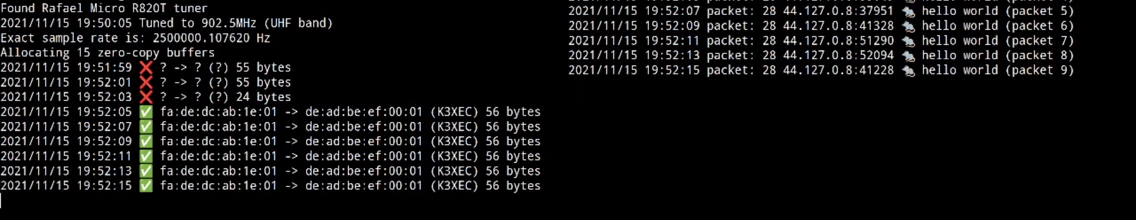
Just an example, I’ve used a custom subpacket to create test vectors, the data is encoded into a Vendor Extension, followed by the IQ for the modulated packet. If the demodulated data and in-band original data don’t match, we’ve regressed. You could imagine in-band speech-to-text, antenna rotator azimuth information, or demodulated digital sideband data (like FM HDR data) too. Or even things I can’t even think of!

id data

In order to help with checking the basic parsing and encoding of this format, the following is a vendor extension subpacket (when encoded or decoded this will be found inside an ARF packet as described above).

// extension id (b24305f6-ff73-4b7a-ae99-7a6b37a5d5cd)
b2, 43, 05, f6, ff, 73, 4b, 7a,
ae, 99, 7a, 6b, 37, a5, d5, cd,

// data (0x01, 0x02, 0x03, 0x04, 0x05)
01, 02, 03, 04, 05

Tradeoffs

The biggest tradeoff that I’m not entirely happy with is limiting the length of a packet to u16 – 65535 bytes. Given the u8 sample header, this limits us to 8191 32 bit sample pairs at a time. I wound up believing that the overhead in terms of additional packet framing is worth it – because always encoding 4 byte lengths felt like overkill, and a dynamic length scheme ballooned codepaths in the decoder that I was trying to keep as easy to change as possible as I worked with the format.

Interested in future updates? Follow me on mastodon at @paul@soylent.green. Posts about hz.tools will be tagged #hztools.

It’s well known and universally agreed that radios are cool. Among the contested field of coolest radios, Software Defined Radios (SDRs) are definitely the most interesting to me. Out of all of my (entirely too many) SDRs I own, the rtlsdr is still my #1. It’s just good. It’s a great price, extremely capable, reliable, well-supported, and compact. Why bother with anything else? Sure, it can’t transmit, uses a (fairly weird) 8 bit unsigned integer IQ representation, limited sampling rate, limited frequency range – but even with all that, it’s still the radio I will pack first. Don’t get me wrong, I love my Ettus radios, PlutoSDRs, HackRFs, my AirspyHF+ - they’re great! I just always find myself falling back to an rtl-sdr, every time.

Perhaps the best reason to use an rtlsdr is the absolutely mind-boggling amount of cool stuff people have written for it. The rtlsdr API is super easy to use, widely supported if you’re building on top of existing radio processing frameworks – it’s still a shock to me when something omits rtlsdr support.

sparky

Over the last 7 years, I’ve been learning about radios – I got my ham radio license (de K3XEC), hacked on some cool stuff where I’ve learned how radios work by “doing”, and even was lucky enough to give my first rf-centric talk at districtcon. Embarrassingly, I still haven’t gotten around to learning how the fancy stuff like GNU Radio works. I’m sure I’m going to love it when I do.

As part of this, I’ve also cooked up some very unprofessional formats and protocols I use for convenience. Locally, all my on-disk captures are stored in rfcap or more recently arf, while direct SDR access at my house is almost entirely a mix of the widely used rtl-tcp protocol, and my “riq” protocol (post on this coming soon). Both rtl-tcp and riq operate over the network, so I don’t have to bother with plugging things into USB ports, and I can share my radios with my friends.

All of that work sits in my current generation of radio processing code, “sparky” (a reference to spark-gap transmitters), which is a heap of Rust, supporting everything from no_std for embedded experiments, conditional support for interfacing with all the radios I own, and tokio-based async support in addition to blocking i/o for highly concurrent daemons. This quickly advanced beyond my old Go-based code (hz.tools/go-sdr), which I archived so I can focus on learning. I still think Go is a great language to write RF code in – but I can’t focus on that tech tree anymore.

Of course, this now poses a new problem – no one supports my format(s) or radio protocol(s), since, well, I’m the only one using them. I’ve committed a fair amount of my hardware to this setup, and yanking it from the rack to try something out does pose a bit of a pickle. This isn’t a huge deal for learning, but it does make it tedious to try out something from the internets.

librtlsdr.so

Thankfully, Rust has robust support for wrap[ping itself] in a grotesque simulacra of C’s skin and mak[ing its] flesh undulate, which is an attractive nuisance if i’ve ever seen one. Naturally, my ability to restrain myself from engaging in ill-advised rf adventures is basically zero, so it’s time to do the thing any similarly situated person would do – reimplement the API and ABI of librtlsdr.so, backed with sparky instead.

Since enumeration of devices is going to be annoying (specifically, they’re over the network), I decided early-on to rely on an explicit list of devices via a configuration file. I’d rather only load that once so programs don’t get confused, so I opted to use a CTOR to run a stub when the ELF is linked at runtime.

// lightly edited for clarity

#[used]
#[expect(unused)]
#[unsafe(link_section = ".init_array")]
pub static INITIALIZE: extern "C" fn() = sparky_rtlsdr_ctor;

#[unsafe(no_mangle)]
pub extern "C" fn sparky_rtlsdr_ctor() {
 let config: Config = {
 if let Ok(config_bytes) = std::fs::read("/etc/sparky-rtlsdr.toml") {
 toml::from_slice(&config_bytes).unwrap()
 } else {
 Config { device: vec![] }
 }
 };
 CONFIG.set(config);
}

Next, it’s time to start with the basics. Opening and closing a handle using rtlsdr_open and rtlsdr_close. Given we don’t control the runtime, and the rtl-sdr device handle is opaque (for good reason!), I opted to smuggle a rust Box<Device> non-FFI safe heap-allocated struct through the device handle pointer, and let C take ownership of the Box. No one should be looking in there anyway.

// lightly edited for clarity

#[unsafe(no_mangle)]
pub unsafe extern "C" fn rtlsdr_open(dev: *mut *mut Handle, index: u32) -> int {
 let config = &CONFIG.device[index as usize];
 let sdr = match config.load() {
 Ok(v) => v,
 Err(err) => {
 return -1;
 }
 };
 let handle = Box::new(Handle { config, sdr });
 unsafe { *dev = Box::into_raw(handle) };
 0
}

#[unsafe(no_mangle)]
pub unsafe extern "C" fn rtlsdr_close(dev: *mut Handle) -> int {
 let dev = unsafe { Box::from_raw(dev) };
 drop(dev);
 0
}

With that in place, we can chip away at the API surface, translating calls as best as we can. I won’t bother listing it all, since it’s not very interesting – but here’s an example implementation of rtlsdr_set_sample_rate and rtlsdr_get_sample_rate. These calls are translating from an rtl-sdr frequency (which is a u32 containing the value as Hz) into a sparky Frequency type, and invoking get_sample_rate or set_sample_rate on the device’s rust handle. Since each device implements the sparky Sdr trait, the actual underlying device doesn’t matter much here.

#[unsafe(no_mangle)]
pub unsafe extern "C" fn rtlsdr_set_sample_rate(dev: *mut Handle, rate: u32) -> int {
 let dev = unsafe { &mut *dev };
 let rate = Frequency::from_hz(rate as i64);
 if let Err(err) = dev.sdr.set_sample_rate(dev.channel, rate) {
 return -1;
 }
 0
}

#[unsafe(no_mangle)]
pub unsafe extern "C" fn rtlsdr_get_sample_rate(dev: *mut Handle) -> u32 {
 let dev = unsafe { &mut *dev };
 let freq = match dev.sdr.get_sample_rate(dev.channel) {
 Ok(freq) => freq,
 Err(err) => {
 return 0;
 }
 };
 freq.as_hz() as u32
}

After repeating this process for the rest of the stubs I could (and otherwise setting error conditions if the functionality is not supported), I was ready to try it out. Within sparky, I patched my “MockSDR” (basically a Sdr traited Mock type) to implement the same testmode IQ protocol that the RTL-SDR has, and decided to see if rtl_test from apt without any changes could be fooled.

$ rtl_test
No supported devices found.

Great, cool. No devices plugged in. Looks great. Let’s try it with my librtlsdr.so LD_PRELOAD-ed into the binary first:

$ LD_PRELOAD=target/release/librtlsdr.so rtl_test
Found 1 device(s):
 0: hz.tools, mock sdr, SN: totally legit no tricks

Using device 0: sparky mock sdr
Supported gain values (0):
Sampling at 2048000 S/s.

Info: This tool will continuously read from the device, and report if
samples get lost. If you observe no further output, everything is fine.

Reading samples in async mode...
^CSignal caught, exiting!

User cancel, exiting...
Samples per million lost (minimum): 0
$

Outstanding. Even more outstandingly, if I change my testmode implementation to skip samples, rtl_test correctly reports the errors – I think it’s showing promise! On to try the real endgame here – let’s have our new librtlsdr.so connect to an rtl-tcp endpoint and see if rtl_fm works:

LD_PRELOAD=target/release/librtlsdr.so \
 rtl_fm -d 1 -s 120k -E deemp -M fm -f 90.9M | \
 ffplay -f s16le -ar 120k -i -
Found 2 device(s):
 0: hz.tools, mock sdr, SN: totally legit no tricks
 1: hz.tools, rtl-tcp, SN: node2.rf.lan:1202

Using device 1: sparky rtltcp node2
Tuner gain set to automatic.
Tuned to 91170000 Hz.
Oversampling input by: 9x.
Oversampling output by: 1x.
Buffer size: 7.59ms
Sampling at 1080000 S/s.
Output at 120000 Hz.

And there it was! Not the best audio quality (mostly due to my inability to correctly read the rtl_fm manpage to tune the filter and downsample/oversampling rates to audio), but it’s definitely passable. I figured I’d try something that was a bit more interesting next – gqrx, since it’s super handy, I use it a ton, and will definitely amuse me to no end. To my surprise and delight, LD_PRELOAD=target/release/librtlsdr.so gqrx wound up running, and I saw my devices pop right up in the setting menu:

Huge. Huge. Amazing. It did crash as soon as I tried to actually use the radio, but after fixing a few dangling bugs in the API surface (and some assumptions I think some underlying gnuradio driver may be making that I need to double check in the code), I was able to get a super solid stream of broadcast fm radio, with gqrx being none the wiser. It thought it was “just” talking to the device it knows as rtl=1.

Nice. I can’t wait to try this with the rest of the rtl-sdr based tools I like having around using my riq protocol next. I don’t think that’ll be worth a post, but hopefully I’ll get around to publishing details on that stack next.

epilogue

Well. That’s it. End of story. A bit anti-climatic, sure. While this new shim will provide me endless minutes of mild amusement, I could see using this to expose my sparky testing utilities via librtlsdr.so – my “mock sdr” driver allows for replaying captures off disk, which could be interesting to make sure that signals are still properly decoded after changes, or instrument performance changes (via SNR, BER, packets observed, etc) on reference samples I have on my NAS. Maybe that’ll come in handy one day!

Truth be told, I’m not sure I actually want to encourage anyone to do this for real (although I think I’ll definitely be using it on my LAN to see what happens). I also don’t have a repo to share – I don’t particularly feel with dealing with the secondary effects of publishing sparky (and sparky-rtlsdr) yet, since i’m still getting my feet under me on the radio aspect of all this.

I’ll be sure to post updates if anything changes with this here (tagged sparky) and at @paul@soylent.green. I can’t wait to post more about some of the odd sidequests (like this one!) i’ve completed over the last few years – I’ve been waiting to feel confident that my work has matured and was withstood the new problems i’ve thrown at it, and it largely has.

It’s my hope that these projects (and this project in particular) has provided a glimpse into the world of software defined radio for my systems friends, and a bit about systems for my radio friends. It’s not all magic, and I hope someone out there feels inclined to have some fun with radios themselves!

After years of thinking about and learning about how radios work, I figured it was high-time to start to more aggressively share the things i’ve been learning. I had a ton of fun at DistrictCon year 0, so it was a pretty natural place to pitch an RF-focused introductory talk.

I was selected for Year 1, and able to give my first ever RF related talk about how to set off restaurant pagers (including one on stage!) by reading and writing IQ directly using a little bit of stdlib only Python.

This talk is based around the work I’ve written about previously (here, here and here), but the “all-in-one” form factor was something I was hoping would help encourage folks out there to take a look under the hood of some of the gear around them.

(In case the iframe above isn’t working, direct link to the YouTube video recording is here)

I’ve posted my slides from the talk at PARCH.pdf to hopefully give folks some time to flip through them directly.

All in all, the session was great – It was truly humbling to see so many folks interested in hearing me talk about radios. I had a bit of an own-goal in picking a 20 minute form-factor, so the talk is paced wrong (it feels like it went way too fast). Hopefully being able to see the slides and pause the video is helpful.

We had a short ad-hoc session after where I brought two sets of pagers and my power switch; but unfortunately we didn’t have anyone who was able to trigger any of the devices on their own (due to a mix of time between sessions and computer set-up). Hopefully it was enough to get folks interested in trying this on their own!

Some of you may remember that I recently felt a bit underwhelmed by the last pager I reverse engineered – the Retekess TD-158, mostly due to how intuitive their design decions were. It was pretty easy to jump to conclusions because they had made some pretty good decisions on how to do things.

I figured I’d spin the wheel again and try a new pager system – this time I went for a SU-68G-10 pager, since I recognized the form factor as another fairly common unit I’ve seen around town. Off to Amazon I went, bought a set, and got to work trying to track down the FCC filings on this model. I eventually found what seemed to be the right make/model, and it, once again, indicated that this system should be operating in the 433 MHz ISM band likely using OOK modulation. So, figured I’d start with the center of the band (again) at 433.92 MHz, take a capture, test my luck, and was greeted with a now very familiar sight.

Same as the last goarounds, except the premable here is a 0 symbol followed by 6-ish symbol durations of no data, followed by 25 bits of a packet. Careful readers will observe 26 symbols above after the preamble – I did too! The last 0 in the screenshot above is not actually a part of the packet – rather, it’s part of the next packet’s preamble. Each packet is packed in pretty tight.

By Hand Demodulation

Going off the same premise as last time, I figured i’d give it a manual demod and see what shakes out (again). This is now the third time i’ve run this play, so check out either of my prior two posts for a better written description of what’s going on here – I’ll skip all the details since i’d just be copy-pasting from those posts into here. Long story short, I demodulated a call for pager 1, call for pager 10, and a power off command.

What Bits Call 1 1101111111100100100000000 Call 101101111111100100010100000 Off 1101111111100111101101110

A few things jump out at me here – the first 14 bits are fixed (in my case, 11011111111001), which means some mix of preamble, system id, or other system-wide constant. Additionally, The last 9 bits also look like they are our pager – the 1 and 10 pager numbers (LSB bit order) jump right out (100000000 and 010100000, respectively). That just leaves the two remaining bits which look to be the “action” – 00 for a “Call”, and 11 for a “Power off”. I don’t super love this since command has two bits rather than one, the base station ID seems really long, and a 9-bit Pager ID is just weird. Also, what is up with that power-off pager id? Weird. So, let’s go and see what we can do to narrow down and confirm things by hand.

Testing bit flips

Rather than call it a day at that, I figure it’s worth a bit of diligence to make sure it’s all correct – so I figured we should try sending packets to my pagers and see how they react to different messages after flipping bits in parts of the packet.

I implemented a simple base station for the pagers using my Ettus B210mini, and threw together a simple OOK modulator and transmitter program which allows me to send specifically crafted test packets on frequency. Implementing the base station is pretty straightforward, because of the modulation of the signal (OOK), it’s mostly a matter of setting a buffer to 1 and 0 for where the carrier signal is on or off timed to the sample rate, and sending that off to the radio. If you’re interested in a more detailed writeup on the steps involved, there’s a bit more in my christmas tree post.

First off, I’d like to check the base id. I want to know if all the bits in what I’m calling the “base id” are truly part of the base station ID, or perhaps they have some other purpose (version, preamble?). I wound up following a three-step process for every base station id:

• Starting with an unmodified call packet for the pager under test:
  • Flip the Nth bit, and transmit the call. See if the pager reacts.
  • Hold “SET”, and pair the pager with the new packet.
  • Transmit the call. See if the pager reacts.
  • After re-setting the ID, transmit the call with the physical base station, see if the pager reacts.
• Starting with an unmodified off packet for the pager system
• Flip the Nth bit, transmit the off, see if the pager reacts.

What wound up happening is that changing any bit in the first 14 bits meant that the packet no longer worked with any pager until it was re-paired, at which point it begun to work again. This likely means the first 14 bits are part of the base station ID – and not static between base stations, or some constant like a version or something. All bits appear to be used.

I repeated the same process with the “command” bits, and found that only 11 and 00 caused the pagers to react for the pager ids i’ve tried.

I repeated this process one last time with the “pager id” bits this time, and found the last bit in the packet isn’t part of the pager ID, and can be either a 1 or a 0 and still cause the pager to react as if it were a 0. This means that the last bit is unknown but it has no impact on either a power off or call, and all messages sent by my base station always have a 0 set. It’s not clear if this is used by anything – likely not since setting a bit there doesn’t result in any change of behavior I can see yet.

Final Packet Structure

After playing around with flipping bits and testing, the final structure I was able to come up with based on behavior I was able to observe from transmitting hand-crafted packets and watching pagers buzz:

base id command pager id ??? Commands

The command section bit comes in two flavors – either a “call” or an “off” command.

Type Id (2 bits) Description Call00Call the pager identified by the id in pager id Off11Request pagers power off, pager id is always 10110111

As for the actual RF PHY characteristics, here’s my best guesses at what’s going on with them:

What Description Center Frequency 433.92 MHz Modulation OOK Symbol Duration 1300us Bits 25 Preamble 325us of carrier, followed by 8800us of no carrier

I’m not 100% on the timings, but they appear to be close enough to work reliably. Same with the center frequency, it’s roughly right but there may be a slight difference i’m missing.

Lingering Questions

This was all generally pretty understandable – another system that had some good decisions, and wasn’t too bad to reverse engineer. This was a bit more fun to do, since there was a bit more ambiguity here, but still not crazy. At least this one was a bit more ambiguous that needed a bit of followup to confirm things, which made it a bit more fun.

I am left with a few questions, though – which I’m kinda interested in understanding, but I’ll likely need a lot more data and/or original source:

Why is the “command” two bits here? This was a bit tough to understand because of the number of bits they have at their disposal – given the one last bit at the end of the packet that doesn’t seem to do anything, there’s no reason this couldn’t have been a 16 bit base station id, and an 8 bit pager id along with a single bit command (call or off).

When sending an “off” – why is power off that bit pattern? Other pager IDs don’t seem to work with “off”, so it has some meaning, but I’m not sure what that is. You press and hold 9 on the physical base station, but the code winds up coming out to 0xED, 237 or maybe -19 if it’s signed. I can’t quite figure out why it’s this value. Are there other codes?

Finally – what’s up with the last bit? Why is it 25 bits and not 24? It must take more work to process something that isn’t 8 bit aligned – and all for something that’s not being used!

It’s been a while since I played with something new – been stuck in a bit of a rut with radios recently - working on refining and debugging stuff I mostly understand for the time being. The other day, I was out getting some food and I idly wondered how the restaurant pager system worked. Idle curiosity gave way to the realization that I, in fact, likely had the means and ability to answer this question, so I bought the first set of the most popular looking restaurant pagers I could find on eBay, figuring it’d be a fun multi-week adventure.

Order up!

I wound up buying a Retekess brand TD-158 Restaurant Pager System (they looked like ones I’d seen before and seemed to be low-cost and popular), and quickly after, had a pack of 10 pagers and a base station in-hand. The manual stated that the radios operated at 433 MHz (cool! can do! Love a good ISM band device), and after taking an initial read through the manual for tips on the PHY, I picked out a few interesting things. First is that the base station ID was limited to 0-999, which is weird because it means the limiting factor is likely the base-10 display on the base station, not the protocol – we need enough bits to store 999 – at least 10 bits. Nothing else seemed to catch my eye, so I figured may as well jump right to it.

Not being the type to mess with success, I did exactly the same thing as I did in my christmas tree post, and took a capture at 433.92MHz since it was in the middle of the band, and immediately got deja-vu. Not only was the signal at 433.92MHz, but throwing the packet into inspectrum gave me the identical plot of the OOK encoding scheme.

Not just similar – identical. The only major difference was the baud rate and bit structure of the packets, and the only minor difference was the existence of what I think is a wakeup preamble packet (of all zeros), rather than a preamble symbol that lasted longer than usual PHY symbol (which makes this pager system a bit easier to work with than my tree, IMHO).

Getting down to work, I took some measurements to determine what the symbol duration was over the course of a few packets, I was able to determine the symbol rate was somewhere around 858 microseconds (0.000858 seconds per symbol), which is a weird number, but maybe I’m slightly off or there’s some larger math I’m missing that makes this number satisfyingly round (internal low cost crystal clock or something? I assume this is some hardware constraint with the pager?)

Anyway, good enough. Moving along, let’s try our hand at a demod – let’s just assume it’s all the same as the chrismas tree post and demod ones and zeros the same way here. That gives us 26 bits:

00001101110000001010001000

Now, I know we need at least 10 bits for the base station ID, some number of bits for the pager ID, and some bits for the command. This was a capture of me hitting “call” from a base station ID of 55 to a pager with the ID of 10, so let’s blindly look for 10 bit chunks with the numbers we’re looking for:

0000110111 0000001010 001000

Jeez. First try. 10 bits for the base station ID (55 in binary is 0000110111), 10 bits for the pager ID (10 in binary is 0000001010), which leaves us with 6 bits for a command (and maybe something else too?) – which is 8 here. Great, cool, let’s work off that being the case and revisit it if we hit bugs.

Besides our data packet, there’s also a “preamble” packet that I’ll add in, in case it’s used for signal detection or wakeup or something – which is fairly easy to do since it’s the same packet structure as the above, just all zeros. Very kind of them to leave it with the same number of bits and encoding scheme – it’s nice that it can live outside the PHY.

Once I got here, I wrote a quick and dirty modulator, and was able to ring up pagers! Unmitigated success and good news – only downside was that it took me a single night, and not the multi-week adventure I was looking for. Well, let’s finish the job and document what we’ve found for the sake of completeness.

Boxing everything up

My best guess on the packet structure is as follows:

base id argument command

For a call or F2 operation, the argument is the Pager’s ID code, but for other commands it’s a value or an enum, depending. Here’s a table of my by-hand demodulation of all the packet types the base station produces:

Type Cmd Id Description Call8Call the pager identified by the id in argument Off60Request any pagers on the charger power off when power is removed, argument is all zero F240Program a pager to the specified Pager ID (in argument) and base station F344Set the reminder duration in seconds specified in argument F448Set the pager's beep mode to the one in argument (0 is disabled, 1 is slow, 2 is medium, 3 is fast) F552Set the pager's vibration mode to the one in argument (0 is disabled, 1 is enabled) Kitchen’s closed for the night

I’m not going to be publishing this code since I can’t think of a good use anyone would have for this besides folks using a low cost SDR and annoying local restaurants; but there’s enough here for folks who find this interesting to try modulating this protocol on their own hardware if they want to buy their own pack of pagers and give it a shot, which I do encourage! It’s fun! Radios are great, and this is a good protocol to hack with – it’s really nice.

All in all, this wasn’t the multi-week adventure I was looking for, this was still a great exercise and a fun reminder that I’ve come a far way from when I’ve started. It felt a lot like cheating since I was able to infer a lot about the PHY because I’d seen it before, but it was still a great time. I may grab a few more restaurant pagers and see if I can find one with a more exotic PHY to emulate next. I mean why not, I’ve already got the thermal printer libraries working 🖨️

Interested in future updates? Follow me on mastodon at @paul@soylent.green. Posts about hz.tools will be tagged #hztools.

If you're on the Fediverse, I'd very much appreciate boosts on my toot!

While working on hz.tools, I started to move my beamforming code from 2-D (meaning, beamforming to some specific angle on the X-Y plane for waves on the X-Y plane) to 3-D. I’ll have more to say about that once I get around to publishing the code as soon as I’m sure it’s not completely wrong, but in the meantime I decided to write a simple simulator to visually check the beamformer against the textbooks. The results were pretty rad, so I figured I’d throw together a post since it’s interesting all on its own outside of beamforming as a general topic.

I figured I’d write this in Rust, since I’ve been using Rust as my primary language over at zoo, and it’s a good chance to learn the language better.

⚠️ This post has some large GIFs

It make take a little bit to load depending on your internet connection. Sorry about that, I'm not clever enough to do better without doing tons of complex engineering work. They may be choppy while they load or something. I tried to compress an ensmall them, so if they're loaded but fuzzy, click on them to load a slightly larger version.

This post won’t cover the basics of how phased arrays work or the specifics of calculating the phase offsets for each antenna, but I’ll dig into how I wrote a simple “simulator” and how I wound up checking my phase offsets to generate the renders below.

Assumptions

I didn’t want to build a general purpose RF simulator, anything particularly generic, or something that would solve for any more than the things right in front of me. To do this as simply (and quickly – all this code took about a day to write, including the beamforming math) – I had to reduce the amount of work in front of me.

Given that I was concerend with visualizing what the antenna pattern would look like in 3-D given some antenna geometry, operating frequency and configured beam, I made the following assumptions:

All anetnnas are perfectly isotropic – they receive a signal that is exactly the same strength no matter what direction the signal originates from.

There’s a single point-source isotropic emitter in the far-field (I modeled this as being 1 million meters away – 1000 kilometers) of the antenna system.

There is no noise, multipath, loss or distortion in the signal as it travels through space.

Antennas will never interfere with each other.

2-D Polar Plots

The last time I wrote something like this, I generated 2-D GIFs which show a radiation pattern, not unlike the polar plots you’d see on a microphone.

These are handy because it lets you visualize what the directionality of the antenna looks like, as well as in what direction emissions are captured, and in what directions emissions are nulled out. You can see these plots on spec sheets for antennas in both 2-D and 3-D form.

Now, let’s port the 2-D approach to 3-D and see how well it works out.

Writing the 3-D simulator

As an EM wave travels through free space, the place at which you sample the wave controls that phase you observe at each time-step. This means, assuming perfectly synchronized clocks, a transmitter and receiver exactly one RF wavelength apart will observe a signal in-phase, but a transmitter and receiver a half wavelength apart will observe a signal 180 degrees out of phase.

This means that if we take the distance between our point-source and antenna element, divide it by the wavelength, we can use the fractional part of the resulting number to determine the phase observed. If we multiply that number (in the range of 0 to just under 1) by tau, we can generate a complex number by taking the cos and sin of the multiplied phase (in the range of 0 to tau), assuming the transmitter is emitting a carrier wave at a static amplitude and all clocks are in perfect sync.

 let observed_phases: Vec<Complex> = antennas
 .iter()
 .map(|antenna| {
 let distance = (antenna - tx).magnitude();
 let distance = distance - (distance as i64 as f64);
 ((distance / wavelength) * TAU)
 })
 .map(|phase| Complex(phase.cos(), phase.sin()))
 .collect();

At this point, given some synthetic transmission point and each antenna, we know what the expected complex sample would be at each antenna. At this point, we can adjust the phase of each antenna according to the beamforming phase offset configuration, and add up every sample in order to determine what the entire system would collectively produce a sample as.

 let beamformed_phases: Vec<Complex> = ...;
 let magnitude = beamformed_phases
 .iter()
 .zip(observed_phases.iter())
 .map(|(beamformed, observed)| observed * beamformed)
 .reduce(|acc, el| acc + el)
 .unwrap()
 .abs();

Armed with this information, it’s straight forward to generate some number of (Azimuth, Elevation) points to sample, generate a transmission point far away in that direction, resolve what the resulting Complex sample would be, take its magnitude, and use that to create an (x, y, z) point at (azimuth, elevation, magnitude). The color attached two that point is based on its distance from (0, 0, 0). I opted to use the Life Aquatic table for this one.

After this process is complete, I have a point cloud of ((x, y, z), (r, g, b)) points. I wrote a small program using kiss3d to render point cloud using tons of small spheres, and write out the frames to a set of PNGs, which get compiled into a GIF.

Now for the fun part, let’s take a look at some radiation patterns!

1x4 Phased Array

The first configuration is a phased array where all the elements are in perfect alignment on the y and z axis, and separated by some offset in the x axis. This configuration can sweep 180 degrees (not the full 360), but can’t be steared in elevation at all.

Let’s take a look at what this looks like for a well constructed 1x4 phased array:

And now let’s take a look at the renders as we play with the configuration of this array and make sure things look right. Our initial quarter-wavelength spacing is very effective and has some outstanding performance characteristics. Let’s check to see that everything looks right as a first test.

Nice. Looks perfect. When pointing forward at (0, 0), we’d expect to see a torus, which we do. As we sweep between 0 and 360, astute observers will notice the pattern is mirrored along the axis of the antennas, when the beam is facing forward to 0 degrees, it’ll also receive at 180 degrees just as strong. There’s a small sidelobe that forms when it’s configured along the array, but it also becomes the most directional, and the sidelobes remain fairly small.

Long compared to the wavelength (1¼ λ)

Let’s try again, but rather than spacing each antenna ¼ of a wavelength apart, let’s see about spacing each antenna 1¼ of a wavelength apart instead.

The main lobe is a lot more narrow (not a bad thing!), but some significant sidelobes have formed (not ideal). This can cause a lot of confusion when doing things that require a lot of directional resolution unless they’re compensated for.

Going from (¼ to 5¼ λ)

The last model begs the question - what do things look like when you separate the antennas from each other but without moving the beam? Let’s simulate moving our antennas but not adjusting the configured beam or operating frequency.

Very cool. As the spacing becomes longer in relation to the operating frequency, we can see the sidelobes start to form out of the end of the antenna system.

2x2 Phased Array

The second configuration I want to try is a phased array where the elements are in perfect alignment on the z axis, and separated by a fixed offset in either the x or y axis by their neighbor, forming a square when viewed along the x/y axis.

Let’s take a look at what this looks like for a well constructed 2x2 phased array:

Let’s do the same as above and take a look at the renders as we play with the configuration of this array and see what things look like. This configuration should suppress the sidelobes and give us good performance, and even give us some amount of control in elevation while we’re at it.

Sweet. Heck yeah. The array is quite directional in the configured direction, and can even sweep a little bit in elevation, a definite improvement from the 1x4 above.

Long compared to the wavelength (1¼ λ)

Let’s do the same thing as the 1x4 and take a look at what happens when the distance between elements is long compared to the frequency of operation – say, 1¼ of a wavelength apart? What happens to the sidelobes given this spacing when the frequency of operation is much different than the physical geometry?

Mesmerising. This is my favorate render. The sidelobes are very fun to watch come in and out of existence. It looks absolutely other-worldly.

Going from (¼ to 5¼ λ)

Finally, for completeness’ sake, what do things look like when you separate the antennas from each other just as we did with the 1x4? Let’s simulate moving our antennas but not adjusting the configured beam or operating frequency.

Very very cool. The sidelobes wind up turning the very blobby cardioid into an electromagnetic dog toy. I think we’ve proven to ourselves that using a phased array much outside its designed frequency of operation seems like a real bad idea.

Future Work

Now that I have a system to test things out, I’m a bit more confident that my beamforming code is close to right! I’d love to push that code over the line and blog about it, since it’s a really interesting topic on its own. Once I’m sure the code involved isn’t full of lies, I’ll put it up on the hztools org, and post about it here and on mastodon.

The asterisk VoIP project has a protocol built-in called “AudioSocket”. AudioSocket is built on top of TCP, streaming int16 values at a sample rate of 8 kHz, neither of those options are configurable (by design). AudioSocket will stream audio from the connected phone to the tcp server, and play audio samples sent from the tcp server to the phone.

This documentation is a work in progress, and a result of source code spelunking or reverse engineering. It may contain errors or outright lies. The names may not match the original name, but it's been documented on a best-effort basis to help future engineering efforts. AudioSocket Packet

Data is exchanged over AudioSocket by framing data into TLV packets. This should be a pretty natural concept for anyone who’s worked on other line encoding schemes like ASN.1, SSH, PGP, or protobuf.

The type is a uint8, length is transmitted as a uint16, and the payload is a variable sized block of data.

The header is encoded using network byte order (big endian). The only field this really matters for is the length field, since the type field is uint8. The payload format is dependent on the type of message.

type length payload

A full list of Commands, and the semantics of their Argument is detailed on the table below.

Command Definition Payload 0x00 Terminate none 0x01 UUID 16-byte UUID encoded as raw bytes. 0x10 Audio Samples variable length buffer of little endian signed 16 bit integers sampled at 8 kHz 0xFF Error byte (see table below)

The most simple (and also shortest) command for AudioSocket is the “Terminate” command, which can be used to indicate that the connection should be tore down, which is a type of 0x00, and no payload (length of 0, no body). This would be encoded as [0x00, 0x00, 0x00].

Well known Error Codes

The length of the Error packet is not defined, and may be any length. According to an AudioSocket Go library (github.com/CyCoreSystems/audiosocket), Asterisk has the following well known error codes (although I can’t seem to find these in the source, if anyone has a link). Given the most common implementation is asterisk, I suspect mandating a 1-byte Error code is not a bad idea.

Code Impl Description 0x01 Asterisk Caller has hung up the Connection 0x02 Asterisk Error forwarding the Frame to the caller 0x04 Asterisk Internal memory allocation error Example Packets

Terminate the connection:

0x00 0x00 0x00

Indicate an error state of 0x11

0xFF 0x00 0x01 0x11

Send 2 audio samples of +1 and -1

0x10 0x00 0x04 0x01 0x00 0xFF 0xFF

Handshake

After a TCP connection is established, the client is expected to send a UUID Packet to the server, which has an application dependent meaning. It could indicate the audio stream to attach to, an identity, or an API key depending on how the server uses it.

After the UUID packet is sent, both the Client and the Server begin to send Audio packets to their peer until the TCP connection is closed, the Terminate command is issued, or an Error packet is sent.

Implementation Notes

Because the aduio stream needs to be very low latency, it’s advisable to set TCP_NODELAY, in order to disable Nagle’s algorithm on the TCP connection. The reason is that we’re sending many small packets with time sensitive audio information which need to be sent right away, even if there is more data to be sent very shortly after.

Additionally, Asterisk specifically will be very upset if you send headers, and reading the body takes more than 5ms, even if there’s a buffer you never exhaust. This state is hard to hit when the audio data is contained in an IP packet, but it’s very easy to trigger when you’re operating under Nagle’s algorithm, since your packet is likely to be split along non-packet boundaries.

Interested in future updates? Follow me on mastodon at @paul@soylent.green. Posts about hz.tools will be tagged #hztools.

If you're on the Fediverse, I'd very much appreciate boosts on my announcement toot!

Ever since 2019, I’ve been learning about how radios work, and trying to learn about using them “the hard way” – by writing as much of the stack as is practical (for some value of practical) myself. I wrote my first “Hello World” in 2018, which was a simple FM radio player, which used librtlsdr to read in an IQ stream, did some filtering, and played the real valued audio stream via pulseaudio. Over 4 years this has slowly grown through persistence, lots of questions to too many friends to thank (although I will try), and the eternal patience of my wife hearing about radios nonstop – for years – into a number of Go repos that can do quite a bit, and support a handful of radios.

I’ve resisted making the repos public not out of embarrassment or a desire to keep secrets, but rather, an attempt to keep myself free of any maintenance obligations to users – so that I could freely break my own API, add and remove API surface as I saw fit. The worst case was to have this project feel like work, and I can’t imagine that will happen if I feel frustrated by PRs that are “getting ahead of me” – solving problems I didn’t yet know about, or bugs I didn’t understand the fix for.

As my rate of changes to the most central dependencies has slowed, i’ve begun to entertain the idea of publishing them. After a bit of back and forth, I’ve decided it’s time to make a number of them public, and to start working on them in the open, as I’ve built up a bit of knowledge in the space, and I and feel confident that the repo doesn’t contain overt lies. That’s not to say it doesn’t contain lies, but those lies are likely hidden and lurking in the dark. Beware.

That being said, it shouldn’t be a surprise to say I’ve not published everything yet – for the same reasons as above. I plan to open repos as the rate of changes slows and I understand the problems the library solves well enough – or if the project “dead ends” and I’ve stopped learning.

Intention behind hz.tools

It’s my sincere hope that my repos help to make Software Defined Radio (SDR) code a bit easier to understand, and serves as an understandable framework to learn with. It’s a large codebase, but one that is possible to sit down and understand because, well, it was written by a single person. Frankly, I’m also not productive enough in my free time in the middle of the night and on weekends and holidays to create a codebase that’s too large to understand, I hope!

I remain wary of this project turning into work, so my goal is to be very upfront about my boundaries, and the limits of what classes of contributions i’m interested in seeing.

Here’s some goals of open sourcing these repos:

• I do want this library to be used to learn with. Please go through it all and use it to learn about radios and how software can control them!
• I am interested in bugs if there’s a problem you discover. Such bugs are likely a great chance for me to fix something I’ve misunderstood or typoed.
• I am interested in PRs fixing bugs you find. I may need a bit of a back and forth to fully understand the problem if I do not understand the bug and fix yet. I hope you may have some grace if it’s taking a long time.

Here’s a list of some anti-goals of open sourcing these repos.

• I do not want this library to become a critical dependency of an important project, since I do not have the time to deal with the maintenance burden. Putting me in that position is going to make me very uncomfortable.
• I am not interested in feature requests, the features have grown as I’ve hit problems, I’m not interested in building or maintaining features for features sake. The API surface should be exposed enough to allow others to experiment with such things out-of-tree.
• I’m not interested in clever code replacing clear code without a very compelling reason.
• I use GNU/Linux (specifically Debian ), and from time-to-time I’ve made sure that my code runs on OpenBSD too. Platforms beyond that will likely not be supported at the expense of either of those two. I’ll take fixes for bugs that fix a problem on another platform, but not damage the code to work around issues / lack of features on other platforms (like Windows).

I’m not saying all this to be a jerk, I do it to make sure I can continue on my journey to learn about how radios work without my full time job becoming maintaining a radio framework single-handedly for other people to use – even if it means I need to close PRs or bugs without merging it or fixing the issue.

With all that out of the way, I’m very happy to announce that the repos are now public under github.com/hztools.

Should you use this?

Probably not. The intent here is not to provide a general purpose Go SDR framework for everyone to build on, although I am keenly aware it looks and feels like it, since that what it is to me. This is a learning project, so for any use beyond joining me in learning should use something like GNU Radio or a similar framework that has a community behind it.

In fact, I suspect most contributors ought to be contributing to GNU Radio, and not this project. If I can encourage people to do so, contribute to GNU Radio! Nothing makes me happier than seeing GNU Radio continue to be the go-to, and well supported. Consider donating to GNU Radio!

hz.tools/rf - Frequency types

The hz.tools/rf library contains the abstract concept of frequency, and some very basic helpers to interact with frequency ranges (such as helpers to deal with frequency ranges, or frequency range math) as well as frequencies and some very basic conversions (to meters, etc) and parsers (to parse values like 10MHz). This ensures that all the hz.tools libraries have a shared understanding of Frequencies, a standard way of representing ranges of Frequencies, and the ability to handle the IO boundary with things like CLI arguments, JSON or YAML.

The git repo can be found at github.com/hztools/go-rf, and is importable as hz.tools/rf.

 // Parse a frequency using hz.tools/rf.ParseHz, and print it to stdout.
 freq := rf.MustParseHz("-10kHz")

 fmt.Printf("Frequency: %s\n", freq+rf.MHz)
 // Prints: 'Frequency: 990kHz'

 // Return the Intersection between two RF ranges, and print
 // it to stdout.
 r1 := rf.Range{rf.KHz, rf.MHz}
 r2 := rf.Range{rf.Hz(10), rf.KHz * 100}

 fmt.Printf("Range: %s\n", r1.Intersection(r2))
 // Prints: Range: 1000Hz->100kHz

These can be used to represent tons of things - ranges can be used for things like the tunable range of an SDR, the bandpass of a filter or the frequencies that correspond to a bin of an FFT, while frequencies can be used for things such as frequency offsets or the tuned center frequency.

hz.tools/sdr - SDR I/O and IQ Types

This… is the big one. This library represents the majority of the shared types and bindings, and is likely the most useful place to look at when learning about the IO boundary between a program and an SDR.

The git repo can be found at github.com/hztools/go-sdr, and is importable as hz.tools/sdr.

This library is designed to look (and in some cases, mirror) the Go io idioms so that this library feels as idiomatic as it can, so that Go builtins interact with IQ in a way that’s possible to reason about, and to avoid reinventing the wheel by designing new API surface. While some of the API looks (and is even called) the same thing as a similar function in io, the implementation is usually a lot more naive, and may have unexpected sharp edges such as concurrency issues or performance problems.

The following IQ types are implemented using the sdr.Samples interface. The hz.tools/sdr package contains helpers for conversion between types, and some basic manipulation of IQ streams.

IQ Format hz.tools Name Underlying Go Type Interleaved uint8 (rtl-sdr) sdr.SamplesU8 [][2]uint8 Interleaved int8 (hackrf, uhd) sdr.SamplesI8 [][2]int8 Interleaved int16 (pluto, uhd) sdr.SamplesI16 [][2]int16 Interleaved float32 (airspy, uhd) sdr.SamplesC64 []complex64

The following SDRs have implemented drivers in-tree.

SDR Format RX/TX State rtl u8 RX Good HackRF i8 RX/TX Good PlutoSDR i16 RX/TX Good rtl kerberos u8 RX Old uhd i16/c64/i8 RX/TX Good airspyhf c64 RX Exp

The following major packages and subpackages exist at the time of writing:

Import What is it? hz.tools/sdr Core IQ types, supporting types and implementations that interact with the byte boundary hz.tools/sdr/rtl sdr.Receiver implementation using librtlsdr. hz.tools/sdr/rtl/kerberos Helpers to enable coherent RX using the Kerberos SDR. hz.tools/sdr/rtl/e4k Helpers to interact with the E4000 RTL-SDR dongle. hz.tools/sdr/fft Interfaces for performing an FFT, which are implemented by other packages. hz.tools/sdr/rtltcp sdr.Receiver implementation for rtl_tcp servers. hz.tools/sdr/pluto sdr.Transceiver implementation for the PlutoSDR using libiio. hz.tools/sdr/uhd sdr.Transceiver implementation for UHD radios, specifically the B210 and B200mini hz.tools/sdr/hackrf sdr.Transceiver implementation for the HackRF using libhackrf. hz.tools/sdr/mock Mock SDR for testing purposes. hz.tools/sdr/airspyhf sdr.Receiver implementation for the AirspyHF+ Discovery with libairspyhf. hz.tools/sdr/internal/simd SIMD helpers for IQ operations, written in Go ASM. This isn’t the best to learn from, and it contains pure go implemtnations alongside. hz.tools/sdr/stream Common Reader/Writer helpers that operate on IQ streams. hz.tools/fftw - hz.tools/sdr/fft implementation

The hz.tools/fftw package contains bindings to libfftw3 to implement the hz.tools/sdr/fft.Planner type to transform between the time and frequency domain.

The git repo can be found at github.com/hztools/go-fftw, and is importable as hz.tools/fftw.

This is the default throughout most of my codebase, although that default is only expressed at the “leaf” package – libraries should not be hardcoding the use of this library in favor of taking an fft.Planner, unless it’s used as part of testing. There are a bunch of ways to do an FFT out there, things like clFFT or a pure-go FFT implementation could be plugged in depending on what’s being solved for.

hz.tools/{fm,am} - analog audio demodulation and modulation

The hz.tools/fm and hz.tools/am packages contain demodulators for AM analog radio, and FM analog radio. This code is a bit old, so it has a lot of room for cleanup, but it’ll do a very basic demodulation of IQ to audio.

The git repos can be found at github.com/hztools/go-fm and github.com/hztools/go-am, and are importable as hz.tools/fm and hz.tools/am.

As a bonus, the hz.tools/fm package also contains a modulator, which has been tested “on the air” and with some of my handheld radios. This code is a bit old, since the hz.tools/fm code is effectively the first IQ processing code I’d ever written, but it still runs and I run it from time to time.

 // Basic sketch for playing FM radio using a reader stream from
 // an SDR or other IQ stream.

 bandwidth := 150*rf.KHz
 reader, err = stream.ConvertReader(reader, sdr.SampleFormatC64)
 if err != nil {
 ...
 }
 demod, err := fm.Demodulate(reader, fm.DemodulatorConfig{
 Deviation: bandwidth / 2,
 Downsample: 8, // some value here depending on sample rate
 Planner: fftw.Plan,
 })
 if err != nil {
 ...
 }
 speaker, err := pulseaudio.NewWriter(pulseaudio.Config{
 Format: pulseaudio.SampleFormatFloat32NE,
 Rate: demod.SampleRate(),
 AppName: "rf",
 StreamName: "fm",
 Channels: 1,
 SinkName: "",
 })
 if err != nil {
 ...
 }

 buf := make([]float32, 1024*64)
 for {
 i, err := demod.Read(buf)
 if err != nil {
 ...
 }
 if i == 0 {
 panic("...")
 }
 if err := speaker.Write(buf[:i]); err != nil {
 ...
 }
 }

hz.tools/rfcap - byte serialization for IQ data

The hz.tools/rfcap package is the reference implementation of the rfcap “spec”, and is how I store IQ captures locally, and how I send them across a byte boundary.

The git repo can be found at github.com/hztools/go-rfcap, and is importable as hz.tools/rfcap.

If you’re interested in storing IQ in a way others can use, the better approach is to use SigMF – rfcap exists for cases like using UNIX pipes to move IQ around, through APIs, or when I send IQ data through an OS socket, to ensure the sample format (and other metadata) is communicated with it.

rfcap has a number of limitations, for instance, it can not express a change in frequency or sample rate during the capture, since the header is fixed at the beginning of the file.

Before you go on: I've been warned off implementing this in practice on a few counts; namely, the space tradeoff isn't worth it, and it's unlikely to correct meaningful errors. I'm going to leave this post up, but please do take the content with a very large grain of salt!

My initial efforts to build a PHY and Data Link layer – from scratch using my own code – have been progressing nicely since the initial BPSK based protocol I’ve documented under the PACKRAT series. As part of that, I’ve been diving deep into FEC, and in particular, LDPC.

I won’t be able to do an overview of LDPC justice in this post – with any luck that’ll come in a later post to come as part of the RATPACK series, so some knowledge is assumed. As such this post is less useful for those looking to learn about LDPC, and a bit more targeted to those who enjoy talking and thinking about FEC.

Hey, heads up! - This post contains extremely unvalidated and back of the napkin quality work without any effort to prove this out generally. Hopefully this work can be of help to others, but please double check anything below if you need it for your own work!

While implementing LDPC, I’ve gotten an encoder and checker working, enough to use LDPC like a checksum. The next big step is to write a Decoder, which can do error correction. The two popular approaches for the actual correction that I’ve seen while reading about LDPC are Belief Propagation, and some class of linear programming that I haven’t dug into yet. I’m not thrilled at how expensive this all is in software, so while implementing the stack I’ve been exploring every shady side ally to try and learn more about how encoders and decoders work, both in theory - and in practice.

Processing an LDPC Message

Checking if a message is correct is fairly straightforward with LDPC (as with encoding, I’ll note). As a quick refresher – given the LDPC H (check) matrix of width N, you can check your message vector (msg) of length N by multiplying H and msg, and checking if the output vector is all zero.

 // scheme contains our G (generator) and
 // H (check) matrices.
 scheme := {G: Matrix{...}, H: Matrix{...}}

 // msg contains our LDPC message (data and
 // check bits).
 msg := Vector{...}

 // N is also the length of the encoded
 // msg vector after check bits have been
 // added.
 N := scheme.G.Width

 // Now, let's generate our 'check' vector.
 ch := Multiply(scheme.H, msg)

We can now see if the message is correct or not:

 // if the ch vector is all zeros, we know
 // that the message is valid, and we don't
 // need to do anything.
 if ch.IsZero() {
 // handle the case where the message
 // is fine as-is.
 return ...
 }

 // Expensive decode here

This is great for getting a thumbs up / thumbs down on the message being correct, but correcting errors still requires pulling the LDPC matrix values from the g (generator) matrix out, building a bipartite graph, and iteratively reprocessing the bit values, until constraints are satisfied and the message has been corrected.

This got me thinking - what is the output vector when it’s not all zeros? Since 1 values in the output vector indicates consistency problems in the message bits as they relate to the check bits, I wondered if this could be used to speed up my LDPC decoder. It appears to work, so this post is half an attempt to document this technique before I put it in my hot path, and half a plea for those who do like to talk about FEC to tell me what name this technique actually is.

k-Bit Brute Forcing

Given that the output Vector’s non-zero bit pattern is set due to the position of errors in the message vector, let’s use that fact to build up a table of k-Bit errors that we can index into.

 // for clarity's sake, the Vector
 // type is being used as the lookup
 // key here, even though it may
 // need to be a hash or string in
 // some cases.
 idx := map[Vector]int{}

 for i := 0; i < N; i++ {
 // Create a vector of length N
 v := Vector{}
 v.FlipBit(i)

 // Now, let's use the generator matrix to encode
 // the data with checksums, and then use the
 // check matrix on the message to figure out what
 // bit pattern results
 ev := Multiply(scheme.H, Multiply(v, scheme.G))

 idx[ev] = i
 }

This can be extended to multiple bits (hence: k-Bits), but I’ve only done one here for illustration. Now that we have our idx mapping, we can now go back to the hot path on Checking the incoming message data:

 // if the ch vector is all zeros, we know
 // that the message is valid, and we don't
 // need to do anything.
 if ch.IsZero() {
 // handle the case where the message
 // is fine as-is.
 return ...
 }

 errIdx, ok := idx[ch]
 if ok {
 msg.FlipBit(errIdx)
 // Verify the LDPC message using
 // H again here.
 return ...
 }

 // Expensive decode here

Since map lookups wind up a heck of a lot faster than message-passing bit state, the hope here is this will short-circuit easy to solve errors for k-Bits, for some value of k that the system memory can tolerate.

Does this work?

Frankly – I have no idea. I’ve written a small program and brute forced single-bit errors in all bit positions using random data to start with, and I’ve not been able to find any collisions in the 1-bit error set, using the LDPC matrix from 802.3an-2006. Even if I was to find a collision for a higher-order k-Bit value, I’m tempted to continue with this approach, and treat each set of bits in the Vector’s bin (like a hash-table), checking the LDPC validity after each bit set in the bin. As long as the collision rate is small enough, it should be possible to correct k-Bits of error faster than the more expensive Belief Propagation approach. That being said, I’m not entirely convinced collisions will be very common, but it’ll take a bit more time working through the math to say that with any confidence.

Have you seen this approach called something official in publications? See an obvious flaw in the system? Send me a tip, please!

AX.25 is a tough protocol to use on UNIX systems. A lot of the support in Linux, specifically, is pretty hard to use, and tends to be built into the reptilian brain of the kernel. KZ3ROX built a userland AX.25 stack called patty, for which I have now built some Go bindings on top of.

Code needed to create AX.25 Sockets via Go can be found at github.com/k3xec/go-patty, and imported by Go source as k3xec.com/patty.

Overview

Clint patty programs (including consumers of this Go library) work by communicating with a userland daemon (pattyd) via a UNIX named socket. That daemon will communicate with a particular radio using a KISS TNC serial device.

The Go bindings implement as many standard Go library interfaces as is practical, allowing for the “plug and play” use of patty (and AX.25) in places where you would expect a network socket (such as TCP) to work, such as Go’s http library.

Example

package main

import (
 "fmt"
 "log"
 "net"
 "os"
 "time"

 "k3xec.com/patty"
)

func main() {
 callsign := "N0CALL-10"

 client, err := patty.Open("patty.sock")
 if err != nil {
 panic(err)
 }

 l, err := client.Listen("ax25", callsign)
 if err != nil {
 panic(err)
 }

 for {
 log.Printf("Listening for requests to %s", l.Addr())
 conn, err := l.Accept()
 if err != nil {
 log.Printf("Error accepting: %s", err)
 continue
 }

 go handle(conn)
 }
}

func handle(c net.Conn) error {
 defer c.Close()
 log.Printf("New connection from %s (local: %s)", c.RemoteAddr(), c.LocalAddr())

 fmt.Fprintf(c, `

Hello! This is Paul's experimental %s node. Feel free
to poke around. Let me know if you spot anything funny.

Five pings are to follow!

`, c.LocalAddr())

 for i := 0; i < 5; i++ {
 time.Sleep(time.Second * 5)
 fmt.Fprintf(c, "Ping!\n")
 }

 return nil
}

🐀 This post is part of a series called "PACKRAT". If this is the first post you've found, it'd be worth reading the intro post first and then looking over all posts in the series.

In the last post, we left off at being able to send and receive PACKRAT frames to and from devices. Since we can transport IPv4 packets over the network, let’s go ahead and see if we can read/write Ethernet frames from a Linux network interface, and on the backend, read and write PACKRAT frames over the air. This has the benefit of continuing to allow Linux userspace tools to work (like cURL, as we’ll try!), which means we don’t have to do a lot of work to implement higher level protocols or tactics to get a connection established over the link.

Given that this post is less RF and more Linuxy, I’m going to include more code snippits than in prior posts, and those snippits are closer to runable Go, but still not complete examples. There’s also a lot of different ways to do this, I’ve just picked the easiest one for me to implement and debug given my existing tooling – for you, you may find another approach easier to implement!

Again, deviation here is very welcome, and since this segment is the least RF centric post in the series, the pace and tone is going to feel different. If you feel lost here, that’s OK. This isn’t the most important part of the series, and is mostly here to give a concrete ending to the story arc. Any way you want to finish your own journey is the best way for you to finish it!

Implement Ethernet conversion code

This assumes an importable package with a Frame struct, which we can use to convert a Frame to/from Ethernet. Given that the PACKRAT frame has a field that Ethernet doesn’t (namely, Callsign), that will need to be explicitly passed in when turning an Ethernet frame into a PACKRAT Frame.

...

// ToPackrat will create a packrat frame from an Ethernet frame.
func ToPackrat(callsign [8]byte, frame *ethernet.Frame) (*packrat.Frame, error) {
 var frameType packrat.FrameType
 switch frame.EtherType {
 case ethernet.EtherTypeIPv4:
 frameType = packrat.FrameTypeIPv4
 default:
 return nil, fmt.Errorf("ethernet: unsupported ethernet type %x", frame.EtherType)
 }

 return &packrat.Frame{
 Destination: frame.Destination,
 Source: frame.Source,
 Type: frameType,
 Callsign: callsign,
 Payload: frame.Payload,
 }, nil
}

// FromPackrat will create an Ethernet frame from a Packrat frame.
func FromPackrat(frame *packrat.Frame) (*ethernet.Frame, error) {
 var etherType ethernet.EtherType
 switch frame.Type {
 case packrat.FrameTypeRaw:
 return nil, fmt.Errorf("ethernet: unsupported packrat type 'raw'")
 case packrat.FrameTypeIPv4:
 etherType = ethernet.EtherTypeIPv4
 default:
 return nil, fmt.Errorf("ethernet: unknown packrat type %x", frame.Type)
 }

 // We lose the Callsign here, which is sad.
 return &ethernet.Frame{
 Destination: frame.Destination,
 Source: frame.Source,
 EtherType: etherType,
 Payload: frame.Payload,
 }, nil
}

Our helpers, ToPackrat and FromPackrat can now be used to transmorgify PACKRAT into Ethernet, or Ethernet into PACKRAT. Let’s put them into use!

Implement a TAP interface

On Linux, the networking stack can be exposed to userland using TUN or TAP interfaces. TUN devices allow a userspace program to read and write data at the Layer 3 / IP layer. TAP devices allow a userspace program to read and write data at the Layer 2 Data Link / Ethernet layer. Writing data at Layer 2 is what we want to do, since we’re looking to transform our Layer 2 into Ethernet’s Layer 2 Frames. Our first job here is to create the actual TAP interface, set the MAC address, and set the IP range to our pre-coordinated IP range.

...

import (
 "net"

 "github.com/mdlayher/ethernet"
 "github.com/songgao/water"
 "github.com/vishvananda/netlink"
)

...
 config := water.Config{DeviceType: water.TAP}
 config.Name = "rat0"
 iface, err := water.New(config)
 ...
 netIface, err := netlink.LinkByName("rat0")
 ...

 // Pick a range here that works for you!
 //
 // For my local network, I'm using some IPs
 // that AMPR (ampr.org) was nice enough to
 // allocate to me for ham radio use. Thanks,
 // AMPR!
 //
 // Let's just use 10.* here, though.
 //
 ip, cidr, err := net.ParseCIDR("10.0.0.1/24")
 ...
 cidr.IP = ip

 err = netlink.AddrAdd(netIface, &netlink.Addr{
 IPNet: cidr,
 Peer: cidr,
 })
 ...

 // Add all our neighbors to the ARP table
 for _, neighbor := range neighbors {
 netlink.NeighAdd(&netlink.Neigh{
 LinkIndex: netIface.Attrs().Index,
 Type: netlink.FAMILY_V4,
 State: netlink.NUD_PERMANENT,
 IP: neighbor.IP,
 HardwareAddr: neighbor.MAC,
 })
 }

 // Pick a MAC that is globally unique here, this is
 // just used as an example!
 addr, err := net.ParseMAC("FA:DE:DC:AB:LE:01")
 ...

 netlink.LinkSetHardwareAddr(netIface, addr)
 ...
 err = netlink.LinkSetUp(netIface)

 var frame = &ethernet.Frame{}
 var buf = make([]byte, 1500)

 for {
 n, err := iface.Read(buf)
 ...
 err = frame.UnmarshalBinary(buf[:n])
 ...
 // process frame here (to come)
 }
...

Now that our network stack can resolve an IP to a MAC Address (via ip neigh according to our pre-defined neighbors), and send that IP packet to our daemon, it’s now on us to send IPv4 data over the airwaves. Here, we’re going to take packets coming in from our TAP interface, and marshal the Ethernet frame into a PACKRAT Frame and transmit it. As with the rest of the RF code, we’ll leave that up to the implementer, of course, using what was built during Part 2: Transmitting BPSK symbols and Part 4: Framing data.

...
 for {
 // continued from above

 n, err := iface.Read(buf)
 ...
 err = frame.UnmarshalBinary(buf[:n])
 ...

 switch frame.EtherType {
 case 0x0800:
 // ipv4 packet
 pack, err := ToPackrat(
 // Add my callsign to all Frames, for now
 [8]byte{'K', '3', 'X', 'E', 'C'},
 frame,
 )
 ...
 err = transmitPacket(pack)
 ...
 }
 }
...

Now that we have transmitting covered, let’s go ahead and handle the receive path here. We’re going to listen on frequency using the code built in Part 3: Receiving BPSK symbols and Part 4: Framing data. The Frames we decode from the airwaves are expected to come back from the call packratReader.Next in the code below, and the exact way that works is up to the implementer.

...
 for {
 // pull the next packrat frame from
 // the symbol stream as we did in the
 // last post
 packet, err := packratReader.Next()
 ...

 // check for CRC errors and drop invalid
 // packets
 err = packet.Check()
 ...

 if bytes.Equal(packet.Source, addr) {
 // if we've heard ourself transmitting
 // let's avoid looping back
 continue
 }

 // create an ethernet frame
 frame, err := FromPackrat(packet)
 ...

 buf, err := frame.MarshalBinary()
 ...

 // and inject it into the tap
 err = iface.Write(buf)
 ...
 }
...

Phew. Right. Now we should be able to listen for PACKRAT frames on the air and inject them into our TAP interface.

Putting it all Together

After all this work – weeks of work! – we can finally get around to putting some real packets over the air. For me, this was an incredibly satisfying milestone, and tied together months of learning!

I was able to start up a UDP server on a remote machine with an RTL-SDR dongle attached to it, listening on the TAP interface’s host IP with my defined MAC address, and send UDP packets to that server via PACKRAT using my laptop, /dev/udp and an Ettus B210, sending packets into the TAP interface.

Now that UDP was working, I was able to get TCP to work using two PlutoSDRs, which allowed me to run the cURL command I pasted in the first post (both simultaneously listen and transmit on behalf of my TAP interface).

It’s my hope that someone out there will be inspired to implement their own Layer 1 and Layer 2 as a learning exercise, and gets the same sense of gratification that I did! If you’re reading this, and at a point where you’ve been able to send IP traffic over your own Layer 1 / Layer 2, please get in touch! I’d be thrilled to hear all about it. I’d love to link to any posts or examples you publish here!

🐀 This post is part of a series called "PACKRAT". If this is the first post you've found, it'd be worth reading the intro post first and then looking over all posts in the series.

In the last post, we we were able to build a functioning Layer 1 PHY where we can encode symbols to transmit, and receive symbols on the other end, we’re now at the point where we can encode and decode those symbols as bits and frame blocks of data, marking them with a Sender and a Destination for routing to the right host(s). This is a “Layer 2” scheme in the OSI model, which is otherwise known as the Data Link Layer. You’re using one to view this website right now – I’m willing to bet your data is going through an Ethernet layer 2 as well as WiFi or maybe a cellular data protocol like 5G or LTE.

Given that this entire exercise is hard enough without designing a complex Layer 2 scheme, I opted for simplicity in the hopes this would free me from the complexity and research that has gone into this field for the last 50 years. I settled on stealing a few ideas from Ethernet Frames – namely, the use of MAC addresses to identify parties, and the EtherType field to indicate the Payload type. I also stole the idea of using a CRC at the end of the Frame to check for corruption, as well as the specific CRC method (crc32 using 0xedb88320 as the polynomial).

Lastly, I added a callsign field to make life easier on ham radio frequencies if I was ever to seriously attempt to use a variant of this protocol over the air with multiple users. However, given this scheme is not a commonly used scheme, it’s best practice to use a nearby radio to identify your transmissions on the same frequency while testing – or use a Faraday box to test without transmitting over the airwaves. I added the callsign field in an effort to lean into the spirit of the Part 97 regulations, even if I relied on a phone emission to identify the Frames.

As an aside, I asked the ARRL for input here, and their stance to me over email was I’d be OK according to the regs if I were to stick to UHF and put my callsign into the BPSK stream using a widely understood encoding (even with no knowledge of PACKRAT, the callsign is ASCII over BPSK and should be easily demodulatable for followup with me). Even with all this, I opted to use FM phone to transmit my callsign when I was active on the air (specifically, using an SDR and a small bash script to automate transmission while I watched for interference or other band users).

Right, back to the Frame:

sync dest source callsign type payload crc

With all that done, I put that layout into a struct, so that we can marshal and unmarshal bytes to and from our Frame objects, and work with it in software.

type FrameType [2]byte

type Frame struct {
 Destination net.HardwareAddr
 Source net.HardwareAddr
 Callsign [8]byte
 Type FrameType
 Payload []byte
 CRC uint32
}

Time to pick some consts

I picked a unique and distinctive sync sequence, which the sender will transmit before the Frame, while the receiver listens for that sequence to know when it’s in byte alignment with the symbol stream. My sync sequence is [3]byte{'U', 'f', '~'} which works out to be a very pleasant bit sequence of 01010101 01100110 01111110. It’s important to have soothing preambles for your Frames. We need all the good energy we can get at this point.

var (
 FrameStart = [3]byte{'U', 'f', '~'}
 FrameMaxPayloadSize = 1500
)

Next, I defined some FrameType values for the type field, which I can use to determine what is done with that data next, something Ethernet was originally missing, but has since grown to depend on (who needs Length anyway? Not me. See below!)

FrameType Description Bytes Raw Bytes in the Payload field are opaque and not to be parsed. [2]byte{0x00, 0x01} IPv4 Bytes in the Payload field are an IPv4 packet. [2]byte{0x00, 0x02}

And finally, I decided on a maximum length of the Payload, and decided on limiting it to 1500 bytes to align with the MTU of Ethernet.

var (
 FrameTypeRaw = FrameType{0, 1}
 FrameTypeIPv4 = FrameType{0, 2}
)

Given we know how we’re going to marshal and unmarshal binary data to and from Frames, we can now move on to looking through the bit stream for our Frames.

Why is there no Length field?

I was initially a bit surprised that Ethernet Frames didn’t have a Length field in use, but the more I thought about it, the more it seemed like a big ole' failure mode without a good implementation outcome. Either the Length is right (resulting in no action and used bits on every packet) or the Length is not the length of the Payload and the driver needs to determine what to do with the packet – does it try and trim the overlong payload and ignore the rest? What if both the end of the read bytes and the end of the subset of the packet denoted by Length have a valid CRC? Which is used? Will everyone agree? What if Length is longer than the Payload but the CRC is good where we detected a lost carrier?

I decided on simplicity. The end of a Frame is denoted by the loss of the BPSK carrier – when the signal is no longer being transmitted (or more correctly, when the signal is no longer received), we know we’ve hit the end of a packet. Missing a single symbol will result in the Frame being finalized. This can cause some degree of corruption, but it’s also a lot easier than doing tricks like bit stuffing to create an end of symbol stream delimiter.

Finding the Frame start in a Symbol Stream

First thing we need to do is find our sync bit pattern in the symbols we’re receiving from our BPSK demodulator. There’s some smart ways to do this, but given that I’m not much of a smart man, I again decided to go for simple instead. Given our incoming vector of symbols (which are still float values) prepend one at a time to a vector of floats that is the same length as the sync phrase, and compare against the sync phrase, to determine if we’re in sync with the byte boundary within the symbol stream.

The only trick here is that because we’re using BPSK to modulate and demodulate the data, post phaselock we can be 180 degrees out of alignment (such that a +1 is demodulated as -1, or vice versa). To deal with that, I check against both the sync phrase as well as the inverse of the sync phrase (both [1, -1, 1] as well as [-1, 1, -1]) where if the inverse sync is matched, all symbols to follow will be inverted as well. This effectively turns our symbols back into bits, even if we’re flipped out of phase. Other techniques like NRZI will represent a 0 or 1 by a change in phase state – which is great, but can often cascade into long runs of bit errors, and is generally more complex to implement. That representation isn’t ambiguous, given you look for a phase change, not the absolute phase value, which is incredibly compelling.

Here’s a notional example of how I’ve been thinking about the phrase sliding window – and how I’ve been thinking of the checks. Each row is a new symbol taken from the BPSK receiver, and pushed to the head of the sliding window, moving all symbols back in the vector by one.

 var (
 sync = []float{ ... }
 buf = make([]float, len(sync))

 incomingSymbols = []float{ ... }
 )

 for _, el := range incomingSymbols {
 copy(buf, buf[1:])
 buf[len(buf)-1] = el
 if compare(sync, buf) {
 // we're synced!
 break
 }
 }

Given the pseudocode above, let’s step through what the checks would be doing at each step:

Buffer Sync Inverse Sync […]float{0,…,0} ❌ […]float{-1,…,-1} ❌ […]float{1,…,1} […]float{0,…,1} ❌ […]float{-1,…,-1} ❌ […]float{1,…,1} [more bits in] ❌ […]float{-1,…,-1} ❌ […]float{1,…,1} […]float{1,…,1} ❌ […]float{-1,…,-1} ✅ […]float{1,…,1}

After this notional set of comparisons, we know that at the last step, we are now aligned to the frame and byte boundary – the next symbol / bit will be the MSB of the 0th Frame byte. Additionally, we know we’re also 180 degrees out of phase, so we need to flip the symbol’s sign to get the bit. From this point on we can consume 8 bits at a time, and re-assemble the byte stream. I don’t know what this technique is called – or even if this is used in real grown-up implementations, but it’s been working for my toy implementation.

Next Steps

Now that we can read/write Frames to and from PACKRAT, the next steps here are going to be implementing code to encode and decode Ethernet traffic into PACKRAT, coming next in Part 5!

🐀 This post is part of a series called "PACKRAT". If this is the first post you've found, it'd be worth reading the intro post first and then looking over all posts in the series.

In the last post, we worked through how to generate a BPSK signal, and hopefully transmit it using one of our SDRs. Let’s take that and move on to Receiving BPSK and turning that back into symbols!

Demodulating BPSK data is a bit more tricky than transmitting BPSK data, mostly due to tedious facts of life such as space, time, and hardware built with compromises because not doing that makes the problem impossible. Unfortunately, it’s now our job to work within our imperfect world to recover perfect data. We need to handle the addition of noise, differences in frequency, clock synchronization and interference in order to recover our information. This makes life a lot harder than when we transmit information, and as a result, a lot more complex.

Coarse Sync

Our starting point for this section will be working from a capture of a number of generated PACKRAT packets as heard by a PlutoSDR at (xz compressed interleaved int16, 2,621,440 samples per second)

Every SDR has its own oscillator, which eventually controls a number of different components of an SDR, such as the IF (if it’s a superheterodyne architecture) and the sampling rate. Drift in oscillators lead to drifts in frequency – such that what one SDR may think is 100MHz may be 100.01MHz for another radio. Even if the radios were perfectly in sync, other artifacts such as doppler time dilation due to motion can cause the frequency to appear higher or lower in frequency than it was transmitted.

All this is a long way of saying, we need to determine when we see a strong signal that’s close-ish to our tuned frequency, and take steps to roughly correct it to our center frequency (in the order of 100s of Hz to kHz) in order to acquire a phase lock on the signal to attempt to decode information contained within.

The easiest way of detecting the loudest signal of interest is to use an FFT. Getting into how FFTs work is out of scope of this post, so if this is the first time you’re seeing mention of an FFT, it may be a good place to take a quick break to learn a bit about the time domain (which is what the IQ data we’ve been working with so far is), frequency domain, and how the FFT and iFFT operations can convert between them.

Lastly, because FFTs average power over the window, swapping phases such that the transmitted wave has the same number of in-phase and inverted-phase symbols the power would wind up averaging to zero. This is not helpful, so I took a tip from Dr. Marc Lichtman’s PySDR project and used complex squaring to drive our BPSK signal into a single detectable carrier by squaring the IQ data. Because points are on the unit circle and at tau/2 (specifically, tau/(2^1) for BPSK, 2^2 for QPSK) angles, and given that squaring has the effect of doubling the angle, and angles are all mod tau, this will drive our wave comprised of two opposite phases back into a continuous wave – effectively removing our BPSK modulation, making it much easier to detect in the frequency domain. Thanks to Tom Bereknyei for helping me with that!

...
 var iq []complex{}
 var freq []complex{}

 for i := range iq {
 iq[i] = iq[i] * iq[i]
 }

 // perform an fft, computing the frequency
 // domain vector in `freq` given the iq data
 // contained in `iq`.
 fft(iq, freq)

 // get the array index of the max value in the
 // freq array given the magnitude value of the
 // complex numbers.
 var binIdx = max(abs(freq))
...

Now, most FFT operations will lay the frequency domain data out a bit differently than you may expect (as a human), which is that the 0th element of the FFT is 0Hz, not the most negative number (like in a waterfall). Generally speaking, “zero first” is the most common frequency domain layout (and generally speaking the most safe assumption if there’s no other documentation on fft layout). “Negative first” is usually used when the FFT is being rendered for human consumption – such as a waterfall plot.

Given that we now know which FFT bin (which is to say, which index into the FFT array) contains the strongest signal, we’ll go ahead and figure out what frequency that bin relates to.

In the time domain, each complex number is the next time instant. In the frequency domain, each bin is a discrete frequency – or more specifically – a frequency range. The bandwidth of the bin is a function of the sampling rate and number of time domain samples used to do the FFT operation. As you increase the amount of time used to perform the FFT, the more precise the FFT measurement of frequency can be, but it will cover the same bandwidth, as defined by the sampling rate.

...
 var sampleRate = 2,621,440

 // bandwidth is the range of frequencies
 // contained inside a single FFT bin,
 // measured in Hz.
 var bandwidth = sampleRate/len(freq)
...

Now that we know we have a zero-first layout and the bin bandwidth, we can compute what our frequency offset is in Hz.

...
 // binIdx is the index into the freq slice
 // containing the frequency domain data.
 var binIdx = 0

 // binFreq is the frequency of the bin
 // denoted by binIdx
 var binFreq = 0

 if binIdx > len(freq)/2 {
 // This branch covers the case where the bin
 // is past the middle point - which is to say,
 // if this is a negative frequency.
 binFreq = bandwidth * (binIdx - len(freq))
 } else {
 // This branch covers the case where the bin
 // is in the first half of the frequency array,
 // which is to say - if this frequency is
 // a positive frequency.
 binFreq = bandwidth * binIdx
 }
...

However, sice we squared the IQ data, we’re off in frequency by twice the actual frequency – if we are reading 12kHz, the bin is actually 6kHz. We need to adjust for that before continuing with processing.

...
 var binFreq = 0

 ...
 // [compute the binFreq as above]
 ...

 // Adjust for the squaring of our IQ data
 binFreq = binFreq / 2
...

Finally, we need to shift the frequency by the inverse of the binFreq by generating a carrier wave at a specific frequency and rotating every sample by our carrier wave – so that a wave at the same frequency will slow down (or stand still!) as it approaches 0Hz relative to the carrier wave.

 var tau = pi * 2

 // ts tracks where in time we are (basically: phase)
 var ts float

 // inc is the amount we step forward in time (seconds)
 // each sample.
 var inc float = (1 / sampleRate)

 // amount to shift frequencies, in Hz,
 // in this case, shift +12 kHz to 0Hz
 var shift = -12,000

 for i := range iq {
 ts += inc
 if ts > tau {
 // not actually needed, but keeps ts within
 // 0 to 2*pi (since it is modulus 2*pi anyway)
 ts -= tau
 }

 // Here, we're going to create a carrier wave
 // at the provided frequency (in this case,
 // -12kHz)
 cwIq = complex(cos(tau*shift*ts), sin(tau*shift*ts))

 iq[i] = iq[i] * cwIq
 }

Now we’ve got the strong signal we’ve observed (which may or may not be our BPSK modulated signal!) close enough to 0Hz that we ought to be able to Phase Lock the signal in order to begin demodulating the signal.

Filter

After we’re roughly in the neighborhood of a few kHz, we can now take some steps to cut out any high frequency components (both positive high frequencies and negative high frequencies). The normal way to do this would be to do an FFT, apply the filter in the frequency domain, and then do an iFFT to turn it back into time series data. This will work in loads of cases, but I’ve found it to be incredibly tricky to get right when doing PSK. As such, I’ve opted to do this the old fashioned way in the time domain.

I’ve – again – opted to go simple rather than correct, and haven’t used nearly any of the advanced level trickery I’ve come across for fear of using it wrong. As a result, our process here is going to be generating a sinc filter by computing a number of taps, and applying that in the time domain directly on the IQ stream.

// Generate sinc taps

func sinc(x float) float {
 if x == 0 {
 return 1
 }
 var v = pi * x
 return sin(v) / v
}

...
 var dst []float
 var length = float(len(dst))

 if int(length)%2 == 0 {
 length++
 }

 for j := range dst {
 i := float(j)
 dst[j] = sinc(2 * cutoff * (i - (length-1)/2))
 }
...

then we apply it in the time domain

...

 // Apply sinc taps to an IQ stream

 var iq []complex

 // taps as created in `dst` above
 var taps []float
 var delay = make([]complex, len(taps))

 for i := range iq {
 // let's shift the next sample into
 // the delay buffer
 copy(delay[1:], delay)
 delay[0] = iq[i]

 var phasor complex
 for j := range delay {
 // for each sample in the buffer, let's
 // weight them by the tap values, and
 // create a new complex number based on
 // filtering the real and imag values.
 phasor += complex(
 taps[j] * real(delay[j]),
 taps[j] * imag(delay[j]),
 )
 }

 // now that we've run this sample
 // through the filter, we can go ahead
 // and scale it back (since we multiply
 // above) and drop it back into the iq
 // buffer.
 iq[i] = complex(
 real(phasor) / len(taps),
 imag(phasor) / len(taps),
 )
 }

...

After running IQ samples through the taps and back out, we’ll have a signal that’s been filtered to the shape of our designed Sinc filter – which will cut out captured high frequency components (both positive and negative).

Astute observers will note that we’re using the real (float) valued taps on both the real and imaginary values independently. I’m sure there’s a way to apply taps using complex numbers, but it was a bit confusing to work through without being positive of the outcome. I may revisit this in the future!

Downsample

Now, post-filter, we’ve got a lot of extra RF bandwidth being represented in our IQ stream at our high sample rate All the high frequency values are now filtered out, which means we can reduce our sampling rate without losing much information at all. We can either do nothing about it and process at the fairly high sample rate we’re capturing at, or we can drop the sample rate down and help reduce the volume of numbers coming our way.

There’s two big ways of doing this; either you can take every Nth sample (e.g., take every other sample to half the sample rate, or take every 10th to decimate the sample stream to a 10th of what it originally was) which is the easiest to implement (and easy on the CPU too), or to average a number of samples to create a new sample.

A nice bonus to averaging samples is that you can trade-off some CPU time for a higher effective number of bits (ENOB) in your IQ stream, which helps reduce noise, among other things. Some hardware does exactly this (called “Oversampling”), and like many things, it has some pros and some cons. I’ve opted to treat our IQ stream like an oversampled IQ stream and average samples to get a marginal bump in ENOB.

Taking a group of 4 samples and averaging them results in a bit of added precision. That means that a stream of IQ data at 8 ENOB can be bumped to 9 ENOB of precision after the process of oversampling and averaging. That resulting stream will be at 1/4 of the sample rate, and this process can be repeated 4 samples can again be taken for a bit of added precision; which is going to be 1/4 of the sample rate (again), or 1/16 of the original sample rate. If we again take a group of 4 samples, we’ll wind up with another bit and a sample rate that’s 1/64 of the original sample rate.

Phase Lock

Our starting point for this section is the same capture as above, but post-coarse sync, filtering downsampling (xz compressed interleaved float32, 163,840 samples per second)

The PLL in PACKRAT was one of the parts I spent the most time stuck on. There’s no shortage of discussions of how hardware PLLs work, or even a few software PLLs, but very little by way of how to apply them and/or troubleshoot them. After getting frustrated trying to follow the well worn path, I decided to cut my own way through the bush using what I had learned about the concept, and hope that it works well enough to continue on.

PLLs, in concept are fairly simple – you generate a carrier wave at a frequency, compare the real-world SDR IQ sample to where your carrier wave is in phase, and use the difference between the local wave and the observed wave to adjust the frequency and phase of your carrier wave. Eventually, if all goes well, that delta is driven as small as possible, and your carrier wave can be used as a reference clock to determine if the observed signal changes in frequency or phase.

In reality, tuning PLLs is a total pain, and basically no one outlines how to apply them to BPSK signals in a descriptive way. I’ve had to steal an approach I’ve seen in hardware to implement my software PLL, with any hope it’s close enough that this isn’t a hazard to learners. The concept is to generate the carrier wave (as above) and store some rolling averages to tune the carrier wave over time. I use two constants, “alpha” and “beta” (which appear to be traditional PLL variable names for this function) which control how quickly the frequency and phase is changed according to observed mismatches. Alpha is set fairly high, which means discrepancies between our carrier and observed data are quickly applied to the phase, and a lower constant for Beta, which will take long-term errors and attempt to use that to match frequency.

This is all well and good. Getting to this point isn’t all that obscure, but the trouble comes when processing a BPSK signal. Phase changes kick the PLL out of alignment and it tends to require some time to get back into phase lock, when we really shouldn’t even be losing it in the first place. My attempt is to generate two predicted samples, one for each phase of our BPSK signal. The delta is compared, and the lower error of the two is used to adjust the PLL, but the carrier wave itself is used to rotate the sample.

 var alpha = 0.1
 var beta = (alpha * alpha) / 2
 var phase = 0.0
 var frequency = 0.0

 ...

 for i := range iq {
 predicted = complex(cos(phase), sin(phase))
 sample = iq[i] * conj(predicted)
 delta = phase(sample)

 predicted2 = complex(cos(phase+pi), sin(phase+pi))
 sample2 = iq[i] * conj(predicted2)
 delta2 = phase(sample2)

 if abs(delta2) < abs(delta) {
 // note that we do not update 'sample'.
 delta = delta2
 }

 phase += alpha * delta
 frequency += beta * delta

 // adjust the iq sample to the PLL rotated
 // sample.
 iq[i] = sample
 }

 ...

If all goes well, this loop has the effect of driving a BPSK signal’s imaginary values to 0, and the real value between +1 and -1.

Average Idle / Carrier Detect

Our starting point for this section is the same capture as above, but post-PLL (xz compressed interleaved float32, 163,840 samples per second)

When we start out, we have IQ samples that have been mostly driven to an imaginary component of 0 and real value range between +1 and -1 for each symbol period. Our goal now is to determine if we’re receiving a signal, and if so, determine if it’s +1 or -1. This is a deceptively hard problem given it spans a lot of other similarly entertaining hard problems. I’ve opted to not solve the hard problems involved and hope that in practice my very haphazard implementation works well enough. This turns out to be both good (not solving a problem is a great way to not spend time on it) and bad (turns out it does materially impact performance). This segment is the one I plan on revisiting, first. Expect more here at some point!

Given that I want to be able to encapsulate three states in the output from this section (our Symbols are no carrier detected (“0”), real value 1 (“1”) or real value -1 ("-1")), which means spending cycles to determine what the baseline noise is to try and identify when a signal breaks through the noise becomes incredibly important.

var idleThreshold
var thresholdFactor = 10

...
 // sigThreshold is used to determine if the symbol
 // is -1, +1 or 0. It's 1.3 times the idle signal
 // threshold.
 var sigThreshold = (idleThreshold * 0.3) + idleThreshold

 // iq contains a single symbol's worth of IQ samples.
 // clock alignment isn't really considered; so we'll
 // get a bad packet if we have a symbol transition
 // in the middle of this buffer. No attempt is made
 // to correct for this yet.
 var iq []complex

 // avg is used to average a chunk of samples in the
 // symbol buffer.
 var avg float

 var mid = len(iq) / 2

 // midNum is used to determine how many symbols to
 // average at the middle of the symbol.
 var midNum = len(iq) / 50

 for j := mid; j < mid+midNum; j++ {
 avg += real(iq[j])
 }
 avg /= midNum

 var symbol float
 switch {
 case avg > sigThreshold:
 symbol = 1
 case avg < -sigThreshold:
 symbol = -1
 default:
 symbol = 0
 // update the idleThreshold using the thresholdFactor
 // to average the idleThreshold over more samples to
 // get a better idea of average noise.
 idleThreshold = (
 (idleThreshold*(thresholdFactor-1) + symbol) \
 / thresholdFactor
 )
 }

 // write symbol to output somewhere
...

Next Steps

Now that we have a stream of values that are either +1, -1 or 0, we can frame / unframe the data contained in the stream, and decode Packets contained inside, coming next in Part 4!

🐀 This post is part of a series called "PACKRAT". If this is the first post you've found, it'd be worth reading the intro post first and then looking over all posts in the series.

In the last post, we worked through what IQ is, and different formats that it may be sent or received in. Let’s take that and move on to Transmitting BPSK using IQ data!

When we transmit and receive information through RF using an SDR, data is traditionally encoded into a stream of symbols which are then used by a program to modulate the IQ stream, and sent over the airwaves.

PACKRAT uses BPSK to encode Symbols through RF. BPSK is the act of modulating the phase of a sine wave to carry information. The transmitted wave swaps between two states in order to convey a 0 or a 1. Our symbols modulate the transmitted sine wave’s phase, so that it moves between in-phase with the SDR’s transmitter and 180 degrees (or π radians) out of phase with the SDR’s transmitter.

The difference between a “Bit” and a “Symbol” in PACKRAT is not incredibly meaningful, and I’ll often find myself slipping up when talking about them. I’ve done my best to try and use the right word at the right stage, but it’s not as obvious where the line between bit and symbol is – at least not as obvious as it would be with QPSK or QAM. The biggest difference is that there are three meaningful states for PACKRAT over BPSK - a 1 (for “In phase”), -1 (for “180 degrees out of phase”) and 0 (for “no carrier”). For my implementation, a stream of all zeros will not transmit data over the airwaves, a stream of all 1s will transmit all “1” bits over the airwaves, and a stream of all -1s will transmit all “0” bits over the airwaves.

We’re not going to cover turning a byte (or bit) into a symbol yet – I’m going to write more about that in a later section. So for now, let’s just worry about symbols in, and symbols out.

Transmitting a Sine wave at 0Hz

If we go back to thinking about IQ data as a precisely timed measurements of energy over time at some particular specific frequency, we can consider what a sine wave will look like in IQ. Before we dive into antennas and RF, let’s go to something a bit more visual.

For the first example, you can see an example of a camera who’s frame rate (or Sampling Rate!) matches the exact number of rotations per second (or Frequency!) of the propeller and it appears to stand exactly still. Every time the Camera takes a frame, it’s catching the propeller in the exact same place in space, even though it’s made a complete rotation.

The second example is very similar, it’s a light strobing (in this case, our sampling rate, since the darkness is ignored by our brains) at the same rate (frequency) as water dropping from a faucet – and the video creator is even nice enough to change the sampling frequency to have the droplets move both forward and backward (positive and negative frequency) in comparison to the faucet.

IQ works the same way. If we catch something in perfect frequency alignment with our radio, we’ll wind up with readings that are the same for the entire stream of data. This means we can transmit a sine wave by setting all of the IQ samples in our buffer to 1+0i, which will transmit a pure sine wave at exactly the center frequency of the radio.

 var sine []complex{}
 for i := range sine {
 sine[i] = complex(1.0, 0.0)
 }

Alternatively, we can transmit a Sine wave (but with the opposite phase) by flipping the real value from 1 to -1. The same Sine wave is transmitted on the same Frequency, except when the wave goes high in the example above, the wave will go low in the example below.

 var sine []complex{}
 for i := range sine {
 sine[i] = complex(-1.0, 0.0)
 }

In fact, we can make a carrier wave at any phase angle and amplitude by using a bit of trig.

 // angle is in radians - here we have
 // 1.5 Pi (0.75 Tau) or 270 degrees.
 var angle = pi * 1.5

 // amplitude controls the transmitted
 // strength of the carrier wave.
 var amplitude = 1.0

 // output buffer as above
 var sine []complex{}

 for i := range sine {
 sine[i] = complex(
 amplitude*cos(angle),
 amplitude*sin(angle),
 )
 }

The amplitude of the transmitted wave is the absolute value of the IQ sample (sometimes called magnitude), and the phase can be computed as the angle (or argument). The amplitude remains constant (at 1) in both cases. Remember back to the airplane propeller or water droplets – we’re controlling where we’re observing the sine wave. It looks like a consistent value to us, but in reality it’s being transmitted as a pure carrier wave at the provided frequency. Changing the angle of the number we’re transmitting will control where in the sine wave cycle we’re “observing” it at.

Generating BPSK modulated IQ data

Modulating our carrier wave with our symbols is fairly straightforward to do – we can multiply the symbol by 1 to get the real value to be used in the IQ stream. Or, more simply - we can just use the symbol directly in the constructed IQ data.

 var sampleRate = 2,621,440
 var baudRate = 1024

 // This represents the number of IQ samples
 // required to send a single symbol at the
 // provided baud and sample rate. I picked
 // two numbers in order to avoid half samples.
 // We will transmit each symbol in blocks of
 // this size.
 var samplesPerSymbol = sampleRate / baudRate
 var samples = make([]complex, samplesPerSymbol)

 // symbol is one of 1, -1 or 0.
 for each symbol in symbols {
 for i := range samples {
 samples[i] = complex(symbol, 0)
 }
 // write the samples out to an output file
 // or radio.
 write(samples)
 }

If you want to check against a baseline capture, here’s 10 example packets at 204800 samples per second.

Next Steps

Now that we can transmit data, we’ll start working on a receive path in Part 3, in order to check our work when transmitting the packets, as well as being able to hear packets we transmit from afar, coming up next in Part 3!!

🐀 This post is part of a series called "PACKRAT". If this is the first post you've found, it'd be worth reading the intro post first and then looking over all posts in the series.

When working with SDRs, information about the signals your radio is receiving are communicated by streams of IQ data. IQ is short for “In-phase” and “Quadrature”, which means 90 degrees out of phase. Values in the IQ stream are complex numbers, so converting them to a native complex type in your language helps greatly when processing the IQ data for meaning.

I won’t get too deep into what IQ is or why complex numbers (mostly since I don’t think I fully understand it well enough to explain it yet), but here’s some basics in case this is your first interaction with IQ data before going off and reading more.

Before we get started — at any point, if you feel lost in this post, it's OK to take a break to do a bit of learning elsewhere in the internet. I'm still new to this, so I'm sure my overview in one paragraph here won't help clarify things too much. This took me months to sort out on my own. It's not you, really! I particularly enjoyed reading visual-dsp.switchb.org when it came to learning about how IQ represents signals, and Software-Defined Radio for Engineers for a more general reference.

Each value in the stream is taken at a precisely spaced sampling interval (called the sampling rate of the radio). Jitter in that sampling interval, or a drift in the requested and actual sampling rate (usually represented in PPM, or parts per million – how many samples out of one million are missing) can cause errors in frequency. In the case of a PPM error, one radio may think it’s 100.1MHz and the other may think it’s 100.2MHz, and jitter will result in added noise in the resulting stream.

A single IQ sample is both the real and imaginary values, together. The complex number (both parts) is the sample. The number of samples per second is the number of real and imaginary value pairs per second.

Each sample is reading the electrical energy coming off the antenna at that exact time instant. We’re looking to see how that goes up and down over time to determine what frequencies we’re observing around us. If the IQ stream is only real-valued measures (e.g., float values rather than complex values reading voltage from a wire), you can still send and receive signals, but those signals will be mirrored across your 0Hz boundary. That means if you’re tuned to 100MHz, and you have a nearby transmitter at 99.9MHz, you’d see it at 100.1MHz. If you want to get an intuitive understanding of this concept before getting into the heavy math, a good place to start is looking at how Quadrature encoders work. Using complex numbers means we can see “up” in frequency as well as “down” in frequency, and understand that those are different signals.

The reason why we need negative frequencies is that our 0Hz is the center of our SDR’s tuned frequency, not actually at 0Hz in nature. Generally speaking, it’s doing loads in hardware (and firmware!) to mix the raw RF signals with a local oscillator to a frequency that can be sampled at the requested rate (fundamentally the same concept as a superheterodyne receiver), so a frequency of ‘-10MHz’ means that signal is 10 MHz below the center of our SDR’s tuned frequency.

The sampling rate dictates the amount of frequency representable in the data stream. You’ll sometimes see this called the Nyquist frequency. The Nyquist Frequency is one half of the sampling rate. Intuitively, if you think about the amount of bandwidth observable as being 1:1 with the sampling rate of the stream, and the middle of your bandwidth is 0 Hz, you would only have enough space to go up in frequency for half of your bandwidth – or half of your sampling rate. Same for going down in frequency.

Float 32 / Complex 64

IQ samples that are being processed by software are commonly processed as an interleaved pair of 32 bit floating point numbers, or a 64 bit complex number. The first float32 is the real value, and the second is the imaginary value.

I#0 Q#0 I#1 Q#1 I#2 Q#2

The complex number 1+1i is represented as 1.0 1.0 and the complex number -1-1i is represented as -1.0 -1.0. Unless otherwise specified, all the IQ samples and pseudocode to follow assumes interleaved float32 IQ data streams.

Example interleaved float32 file (10Hz Wave at 1024 Samples per Second)

RTL-SDR

IQ samples from the RTL-SDR are encoded as a stream of interleaved unsigned 8 bit integers (uint8 or u8). The first sample is the real (in-phase or I) value, and the second is the imaginary (quadrature or Q) value. Together each pair of values makes up a complex number at a specific time instant.

I#0 Q#0 I#1 Q#1 I#2 Q#2

The complex number 1+1i is represented as 0xFF 0xFF and the complex number -1-1i is represented as 0x00 0x00. The complex number 0+0i is not easily representable – since half of 0xFF is 127.5.

Complex Number Representation 1+1i []uint8{0xFF, 0xFF} -1+1i []uint8{0x00, 0xFF} -1-1i []uint8{0x00, 0x00} 0+0i []uint8{0x80, 0x80} or []uint8{0x7F, 0x7F}

And finally, here’s some pseudocode to convert an rtl-sdr style IQ sample to a floating point complex number:

...
 in = []uint8{0x7F, 0x7F}
 real = (float(iq[0])-127.5)/127.5
 imag = (float(iq[1])-127.5)/127.5
 out = complex(real, imag)
....

Example interleaved uint8 file (10Hz Wave at 1024 Samples per Second)

HackRF

IQ samples from the HackRF are encoded as a stream of interleaved signed 8 bit integers (int8 or i8). The first sample is the real (in-phase or I) value, and the second is the imaginary (quadrature or Q) value. Together each pair of values makes up a complex number at a specific time instant.

I#0 Q#0 I#1 Q#1 I#2 Q#2

Formats that use signed integers do have one quirk due to two’s complement, which is that the smallest negative number representable’s absolute value is one more than the largest positive number. int8 values can range between -128 to 127, which means there’s bit of ambiguity in how +1, 0 and -1 are represented. Either you can create perfectly symmetric ranges of values between +1 and -1, but 0 is not representable, have more possible values in the negative range, or allow values above (or just below) the maximum in the range to be allowed.

Within my implementation, my approach has been to scale based on the max integer value of the type, so the lowest possible signed value is actually slightly smaller than -1. Generally, if your code is seeing values that low the difference in step between -1 and slightly less than -1 isn’t very significant, even with only 8 bits. Just a curiosity to be aware of.

Complex Number Representation 1+1i []int8{127, 127} -1+1i []int8{-128, 127} -1-1i []int8{-128, -128} 0+0i []int8{0, 0}

And finally, here’s some pseudocode to convert a hackrf style IQ sample to a floating point complex number:

...
 in = []int8{-5, 112}
 real = (float(in[0]))/127
 imag = (float(in[1]))/127
 out = complex(real, imag)
....

Example interleaved int8 file (10Hz Wave at 1024 Samples per Second)

PlutoSDR

IQ samples from the PlutoSDR are encoded as a stream of interleaved signed 16 bit integers (int16 or i16). The first sample is the real (in-phase or I) value, and the second is the imaginary (quadrature or Q) value. Together each pair of values makes up a complex number at a specific time instant.

Almost no SDRs capture at a 16 bit depth natively, often you’ll see 12 bit integers (as is the case with the PlutoSDR) being sent around as 16 bit integers. This leads to the next possible question, which is are values LSB or MSB aligned? The PlutoSDR sends data LSB aligned (which is to say, the largest real or imaginary value in the stream will not exceed 4095), but expects data being transmitted to be MSB aligned (which is to say the lowest set bit possible is the 5th bit in the number, or values can only be set in increments of 16).

As a result, the quirk observed with the HackRF (that the range of values between 0 and -1 is different than the range of values between 0 and +1) does not impact us so long as we do not use the whole 16 bit range.

Complex Number Representation 1+1i []int16{32767, 32767} -1+1i []int16{-32768, 32767} -1-1i []int16{-32768, -32768} 0+0i []int16{0, 0}

And finally, here’s some pseudocode to convert a PlutoSDR style IQ sample to a floating point complex number, including moving the sample from LSB to MSB aligned:

...
 in = []int16{-15072, 496}
 // shift left 4 bits (16 bits - 12 bits = 4 bits)
 // to move from LSB aligned to MSB aligned.
 in[0] = in[0] << 4
 in[1] = in[1] << 4

 real = (float(in[0]))/32767
 imag = (float(in[1]))/32767
 out = complex(real, imag)
....

Example interleaved i16 file (10Hz Wave at 1024 Samples per Second)

Next Steps

Now that we can read (and write!) IQ data, we can get started first on the transmitter, which we can (in turn) use to test receiving our own BPSK signal, coming next in Part 2!

Hello! Welcome. I’m so thrilled you’re here.

Some of you may know this (as I’ve written about in the past), but if you’re new to my RF travels, I’ve spent nights and weekends over the last two years doing some self directed learning on how radios work. I’ve gone from a very basic understanding of wireless communications, all the way through the process of learning about and implementing a set of libraries to modulate and demodulate data using my now formidable stash of SDRs. I’ve been implementing all of the RF processing code from first principals and purely based on other primitives I’ve written myself to prove to myself that I understand each concept before moving on.

I’ve just finished a large personal milestone – I was able to successfully send a cURL HTTP request through a network interface into my stack of libraries, through my own BPSK implementation, framed in my own artisanal hand crafted Layer 2 framing scheme, demodulated by my code on the other end, and sent into a Linux network interface. The combination of the Layer 1 PHY and Layer 2 Data Link is something that I’ve been calling “PACKRAT”.

$ curl http://44.127.0.8:8000/
* Connected to 44.127.0.8 (44.127.0.8) port 8000 (#0)
> GET / HTTP/1.1
> Host: localhost:1313
> User-Agent: curl/7.79.1
> Accept: */*
>
* Mark bundle as not supporting multiuse
* HTTP/1.0, assume close after body
< HTTP/1.0 200 OK
< Content-Length: 236
<



 ____ _ ____ _ ______ _ _____
| _ \ / \ / ___| |/ / _ \ / \|_ _|
| |_) / _ \| | | ' /| |_) | / _ \ | |
| __/ ___ \ |___| . \| _ < / ___ \| |
|_| /_/ \_\____|_|\_\_| \_\/_/ \_\_|



* Closing connection 0

In an effort to “pay it forward” to thank my friends for their time walking me through huge chunks of this, and those who publish their work, I’m now spending some time documenting how I was able to implement this protocol. I would never have gotten as far as I did without the incredible patience and kindness of friends spending time working with me, and educators publishing their hard work for the world to learn from. Please accept my deepest thanks and appreciation.

The PACKRAT posts are written from the perspective of a novice radio engineer, but experienced software engineer. I’ll be leaving out a lot of the technical details on the software end and specific software implementation, focusing on the general gist of the implementation in the radio critical components exclusively. The idea here is this is intended to be a framework – a jumping off point – for those who are interested in doing this themselves. I hope that this series of blog posts will come to be useful to those who embark on this incredibly rewarding journey after me.

This is the first post in the series, and it will contain links to all the posts to follow. This is going to be the landing page I link others to – as I publish additional posts, I’ll be updating the links on this page. The posts will also grow a tag, which you can check back on, or follow along with here.

Tau

Tau (𝜏) is a much more natural expression of the mathematical constant used for circles which I use rather than Pi (π). You may see me use Tau in code or text – Tau is the same as 2π, so if you see a Tau and don’t know what to do, feel free to mentally or textually replace it with 2π. I just hate always writing 2π everywhere – and only using π (or worse yet – 2π/2) .when I mean 1/2 of a circle (or, 𝜏/2).

Pseudo-code

Basically none of the code contained in this series is valid on its own. It’s very lightly basically Go, and only meant to express concepts in term of software. The examples in the post shouldn’t be taken on their own as working snippits to process IQ data, but rather, be used to guide implementations to process the data in question. I’d love to invite all readers to try to “play at home” with the examples, and try and work through the example data captures!

Captures

Speaking of captures, I’ve included live on-the-air captures of PACKRAT packets, as transmitted from my implementation, in different parts of these posts. This means you can go through the process of building code to parse and receive PACKRAT packets, and then build a transmitter that is validated by your receiver. It’s my hope folks will follow along at home and experiment with software to process RF data on their own!

Posts in this series

• Part 1: Processing IQ data
• Part 2: Transmitting BPSK symbols
• Part 3: Receiving BPSK symbols
• Part 4: Framing data
• Part 5: Proxying Ethernet Frames to PACKRAT

Over the last few years, I’ve often wondered what the true power output of my SDRs are. It’s a question with a shocking amount of complexity in the response, due to a number of factors (mostly Frequency). The ranges given in spec sheets are often extremely vague, and if I’m being honest with myself, not incredibly helpful for being able to determine what specific filters and amplifiers I’ll need to get a clean signal transmitted.

Hey, heads up! - This post contains extremely unvalidated and back of the napkin quality work to understand how my equipment works. Hopefully this work can be of help to others, but please double check any information you need for your own work!

I was specifically interested in what gain output (in dBm) looks like across the frequency range – in particular, how variable the output dBm is when I change frequencies. The second question I had was understanding how linear the output gain is when adjusting the requested gain from the radio. Does a 2 dB increase on a HackRF API mean 2 dB of gain in dBm, no matter what the absolute value of the gain stage is?

I’ve finally bit the bullet and undertaken work to characterize the hardware I do have, with some outdated laboratory equipment I found on eBay. Of course, if it’s worth doing, it’s worth overdoing, so I spent a bit of time automating a handful of components in order to collect the data that I need from my SDRs.

I bought an HP 437B, which is the cutting edge of 30 years ago, but still accurate to within 0.01dBm. I paired this Power Meter with an Agilent 8481A Power Sensor (-30 dBm to 20 dBm from 10MHz to 18GHz). For some of my radios, I was worried about exceeding the 20 dBm mark, so I used a 20db attenuator while I waited for a higher power power sensor. Finally, I was able to find a GPIB to USB interface, and get that interface working with the GPIB Kernel driver on my system.

With all that out of the way, I was able to write Go bindings to my HP 437B to allow for totally headless and automated control in sync with my SDR’s RF output. This allowed me to script the transmission of a sine wave at a controlled amplitude across a defined gain range and frequency range and read the Power Sensor’s measured dBm output to characterize the Gain across frequency and configured Gain.

HackRF

Looking at configured Gain against output power, the requested gain appears to have a fairly linear relation to the output signal power. The measured dBm ranged between the sensor noise floor to approx +13dBm. The average standard deviation of all tested gain values over the frequency range swept was +/-2dBm, with a minimum standard deviation of +/-0.8dBm, and a maximum of +/-3dBm.

When looking at output power over the frequency range swept, the HackRF contains a distinctive (and frankly jarring) ripple across the Frequency range, with a clearly visible jump in gain somewhere around 2.1GHz. I have no idea what is causing this massive jump in output gain, nor what is causing these distinctive ripples. I’d love to know more if anyone’s familiar with HackRF’s RF internals!

PlutoSDR

The power output is very linear when operating above -20dB TX channel gain, but can get quite erratic the lower the output power is configured. The PlutoSDR’s output power is directly related to the configured power level, and is generally predictable once a minimum power level is reached. The measured dBm ranged from the noise floor to 3.39 dBm, with an average standard deviation of +/-1.98 dBm, a minimum standard deviation of +/-0.91 dBm and a maximum standard deviation of +/-3.37 dBm.

Generally, the power output is quite stable, and looks to have very even and wideband gain control. There’s a few artifacts, which I have not confidently isolated to the SDR TX gain, noise (transmit artifacts such as intermodulation) or to my test setup. They appear fairly narrowband, so I’m not overly worried about them yet. If anyone has any ideas what this could be, I’d very much appreciate understanding why they exist!

Ettus B210

The power output on the Ettus B210 is higher (in dBm) than any of my other radios, but it has a very odd quirk where the power becomes nonlinear somewhere around -55dB TX channel gain. After that point, adding gain has no effect on the measured signal output in dBm up to 0 dB gain. The measured dBm ranged from the noise floor to 18.31 dBm, with an average standard deviation of +/-2.60 dBm, a minimum of +/-1.39 dBm and a maximum of +/-5.82 dBm.

When the Gain is somewhere around the noise floor, the measured gain is incredibly erratic, which throws the maximum standard deviation significantly. I haven’t isolated that to my test setup or the radio itself. I’m inclined to believe it’s my test setup. The radio has a fairly even and wideband gain, and so long as you’re operating between -70dB to -55dB, fairly linear as well.

Summary

Of all my radios, the Ettus B210 has the highest output (in dBm) over the widest frequency range, but the HackRF is a close second, especially after the gain bump kicks in around 2.1GHz. The Pluto SDR feels the most predictable and consistent, but also a very low output, comparatively - right around 0 dBm.

Name Max dBm stdev dBm stdev min dBm stdev max dBm HackRF +12.6 +/-2.0 +/-0.8 +/-3.0 PlutoSDR +3.3 +/-2.0 +/-0.9 +/-3.7 B210 +18.3 +/-2.6 +/-1.4 +/-6.0

Over the course of the last year and a half, I’ve been doing some self-directed learning on how radios work. I’ve gone from a very basic understanding of wireless communications (there’s usually some sort of antenna, I guess?) all the way through the process of learning about and implementing a set of libraries to modulate and demodulate data using my now formidable stash of SDRs. I’ve been implementing all of the RF processing code from first principals and purely based on other primitives I’ve written myself to prove to myself that I understand each concept before moving on.

I figured that there was a fun “capstone” to be done here - the blind reverse engineering and implementation of the protocol my cheep Amazon power switch uses to turn on and off my Christmas Tree. All the work described in this post was done over the course of a few hours thanks to help during the demodulation from Tom Bereknyei and hlieberman.

Going in blind

When I first got my switch, I checked it for any FCC markings in order to look up the FCC filings to determine the operational frequency of the device, and maybe some other information such as declared modulation or maybe even part numbers and/or diagrams. However, beyond a few regulatory stickers, there were no FCC ids or other distinguishing IDs on the device. Worse yet, it appeared to be a whitelabeled version of another product, so searching Google for the product name was very unhelpful.

Since operation of this device is unlicensed, I figured I’d start looking in the ISM band. The most common band used that I’ve seen is the band starting at 433.05MHz up to 434.79MHz. I fired up my trusty waterfall tuned to a center frequency of 433.92MHz (since it’s right in the middle of the band, and it let me see far enough up and down the band to spot the remote) and pressed a few buttons. Imagine my surprise when I realize the operational frequency of this device is 433.920MHz, exactly dead center. Weird, but lucky!

After taking a capture, I started to look at understanding what the modulation type of the signal was, and how I may go about demodulating it. Using inspectrum, I was able to clearly see the signal in the capture, and it immediately stuck out to my eye to be encoded using OOK / ASK.

Next, I started to measure the smallest pulse, and see if I could infer the symbols per second, and try to decode it by hand. These types of signals are generally pretty easy to decode by eye.

This wound up giving me symbol rate of 2.2 Ksym/s, which is a lot faster than I expected. While I was working by hand, Tom demodulated a few messages in Python, and noticed that if you grouped the bits into groups of 4, you either had a 1000 or a 1110 – which caused me to realize this was encoded using something I saw documented elsewhere, where the 0 is a “short” pulse, and a 1 is a “long” pulse, not unlike morse code, but where each symbol takes up a fixed length of time (monospace morse code?). Working on that assumption, I changed my inspectrum symbol width, and demodulated a few more by hand. This wound up demodulating nicely (and the preamble / clock sync could be represented as repeating 0s, which is handy!) and gave us a symbol rate of 612(ish) symbols per second – a lot closer to what I was expecting.

If we take the code for ‘on’ in the inspectrum capture above and demodulate it by hand, we get 0000000000110101100100010 (treat a short pulse as a 0, and a long pulse as a 1). If you’re interested in following along at home, click on the inspectrum image, and write down the bits you see, and compare it to what I have!

Right, so it looks like from what we can tell so far that the packet looks something like this:

preamble / sync stuff

Next, I took a capture of all the button presses and demodulated them by hand, and put them into a table to try and understand the format of the messages:

Button Demod'd Bits On 0000000000110101100100010 Off 00000000001101011001010000 Dim Up 0000000000110101100110100 Dim Down 0000000000110101100100100 Timer 1h 0000000000110101100110010 Timer 2h 0000000000110101100100110 Timer 4h 0000000000110101100100000 Dim 100% 0000000000110101000101010 Dim 75% 00000000001101010001001100 Dim 50% 00000000001101010001001000 Dim 25% 0000000000110101000100000

Great! So, this is enough to attempt to control the tree with, I think – so I wrote a simple modulator. My approach was to use the fact that I can break down a single symbol into 4 “sub-symbol” components – which is to say, go back to representing a 1 as 1110, and a 0 as 1000. This let me allocate IQ space for the symbol, break the bit into 4 symbols, and if that symbol is 1, write out values from a carrier wave (cos in the real values, and sin in the imaginary values) to the buffer. Now that I can go from bits to IQ data, I can transmit that IQ data using my PlutoSDR or HackRF and try and control my tree. I gave it a try, and the tree blinked off!

🎉🎊 Success! 🎊🎉

But wait – that’s not enough for me – I know I can’t just demodulate bits and try and replay the bits forever – there’s stuff like addresses and keys and stuff, and I want to get a second one of these working. Let’s take a look at the bits to see if we spot anything fun & interesting.

At first glance, a few things jumped out at me as being… weird? First is that the preamble is 10 bits long (fine, let’s move along - maybe it just needs 8 in a row and there’s two to ensure clocks sync?). Next is that the messages are not all the same length. I double (and triple!) checked the messages, and it’s true, the messages are not all the same length. Adding an extra bit at the end didn’t break anything, but I wonder if that’s just due to the implementation rather than the protocol.

But, good news, it looks like we have a stable prefix to the messages from the remote – must be my device’s address! The stable 6 bits that jump out right away are 110101. Something seems weird, though, 6 bits is a bit awkward, even for a bit limited embedded device. Why 6? But hey, wait, we had 10 bits in the preamble, what if we have an 8 bit address – meaning my device is 00110101, and the preamble is 8 0 symbols! Those are numbers that someone working on an 8 bit aligned platform would pick! To test this, I added a 0 to the preamble to see if the message starts at the first 1, or if it requires all the bits to be fully decoded, and lo and behold, the tree did not turn on or off. This would seem to me to confirm that the 0s are part of the address, and I can assume we have two 8 bit aligned bytes in the prefix of the message.

preamble / sync address stuff

Now, when we go through the 9-10 bits of “stuff”, we see all sorts of weird bits floating all over the place. The first 4 bits look like it’s either 1001 or 0001, but other than that, there’s a lot of chaos. This is where things get really squishy. I needed more information to try and figure this out, but no matter how many times I sent a command it was always the same bits (so, no counters), and things feel very opaque still.

The only way I was going to make any progress is to get another switch and see how the messages from the remote change. Off to Amazon I went, and ordered another switch from the same page, and eagerly waited its arrival.

Switch #2

The second switch showed up, and I hurriedly unboxed the kit, put batteries into the remote, and fired up my SDR to take a capture. After I captured the first button (“Off”), my heart sunk as I saw my lights connected to Switch #1 flicker off. Apparently the new switch and the old switch have the same exact address. To be sure, I demodulated the messages as before, and came out with the exact same bit pattern. This is a setback and letdown – I was hoping to independently control my switches, but it also means I got no additional information about the address or button format.

The upside to all of this, though, is that because the switches are controlled by either remote, I only needed one remote, so why not pull it apart and see if I can figure out what components it’s using to transmit, and find any datasheets I can. The PCB was super simple, and I wound up finding a “WL116SC” IC on the PCB.

After some googling, I found a single lone datasheet, entirely in Chinese. Thankfully, Google Translate seems to have worked well enough on technical words, and I was able to put together at least a little bit of understanding based on the documentation that was made available. I took a few screenshots below - I put the google translated text above the hanzi. From that sheet, we can see we got the basics of the “1” and “0” symbol encoding right (I was halfway expecting the bits to be flipped), and a huge find by way of a description of the bits in the message!

It’s a bummer that we missed the clock sync / preamble pulse before the data message, but that’s OK somehow. It also turns out that 8 or 10 bit series of of “0"s wasn’t clock sync at all - it was part of the address! Since it also turns out that all devices made by this manufacturer have the hardcoded address of []byte{0x00, 0x35}, that means that the vast majority of bits sent are always going to be the same for any button press on any remote made by this vendor. Seems like a waste of bits to me, but hey, what do I know.

Additionally, this also tells us the trailing zeros are not part of the data encoding scheme, which is progress!

address keycode

Now, working on the assumptions validated by the datasheet, here’s the updated list of scancodes we’ve found:

Button Scancode Bits Integer On 10010001 145 / 0x91 Off 10010100 148 / 0x94 Dim Up 10011010 154 / 0x9A Dim Down 10010010 146 / 0x92 Timer 1h 10011001 154 / 0x99 Timer 2h 10010011 147 / 0x93 Timer 4h 10010000 144 / 0x90 Dim 100% 00010101 21 / 0x15 Dim 75% 00010011 19 / 0x13 Dim 50% 00010010 18 / 0x12 Dim 25% 00010000 16 / 0x10

Interestingly, I think the “Dim” keys may have a confirmation that we have a good demod – the codes on the bottom are missing the most significant bit, and when I look back at the scancode table in the datasheet, they make an interesting pattern – the bottom two rows, right and left side values match up! If you take a look, Dim 100% is “S1”, Dim 75% is “S19”, Dim 50% is “S8”, and Dim 25% is “S20”. Cool!

Since none of the other codes line up, I am willing to bet the most significant bit is a “Combo” indicator, and not part of the button (leaving 7 bits for the keycode).

And even more interestingly, one of our scancodes (“Off”, which is 0x94) shows up just below this table, in the examples.

Over all, I think this tells us we have the right bits to look at for determining the scan code! Great news there!

Back to the modulation!

So, armed with this knowledge, I was able to refactor my code to match the timings and understanding outlined by the datasheet and ensure things still work. The switch itself has a high degree of tolerance, so being wildly off frequency or a wildly wrong symbol rate may actually still work. It’s hard to know if this is more or less correct, but matching documentation seems like a more stable foundation if nothing else.

This code has been really reliable, and tends to work just as well as the remote from what I’ve been able to determine. I’ve been using incredibly low power to avoid any interference, and it’s been very robust - a testament to the engineering that went into the outlet hardware, even though it cost less than of a lot of other switches! I have a lot of respect for the folks who built this device - it’s incredibly simple, reliable and my guess is this thing will keep working even in some fairly harsh RF environments.

The only downside is the fact the manufacturer used the same address for all their devices, rather than programming a unique address for each outlet and remote when the underlying WL116SC chip supports it. I’m sure this was done to avoid complexity in assembly (e.g. pairing the remote and outlet, and having to keep those two items together during assembly), but it’s still a bummer. I took apart the switch to see if I could dump an EEPROM and change the address in ROM, but the entire thing was potted in waterproof epoxy, which is a very nice feature if this was ever used outdoors. Not good news for tinkering, though!

Unsolved Mysteries

At this point, even though I understand the protocol enough to control the device, it still feels like I hit a dead end in my understanding. I’m not able to figure out how exactly the scancodes are implemented, and break them down into more specific parts. They are stable and based on the physical wiring of the remote, so I think I’m going to leave it a magic number. I have what I was looking for, and these magic constants appear to be the right one to use, even if I did understand how to create the codes itself.

This does leave us with a few bits we never resolved, which I’ll memorialize below just to be sure I don’t forget about them.

Question #1: According to the datasheet there should be a preamble. Why do I not see one leading the first message?

My hunch is that the trailing “0” at the end of the payload is actually just the preamble for the next message (always rendering the first message invalid?). This would let us claim there’s an engineering reason why we are ignoring the weird bit, and also explain away something from the documentation. It’s just weird that it wouldn’t be present on the first message.

This theory is mostly confirmed by measuring the timing and comparing it to the datasheet, but it’s not exactly in line with the datasheet timings either (specifically, it’s off by 200µs, which is kinda a lot for a system using 400µs timings). I think I could go either way on the last “0” being the preamble for the next message. It could be that the first message is technically invalid, or it could also be that this was not implemented or actively disabled by the vendor for this specific application / device. It’s really hard to know without getting the source code for the WL116SC chip in this specific remote or the source in the outlet itself.

Question #2: Why are some keycodes 8 bits and others 9 bits?

I still have no idea why there sometimes 8 bits (for instance, “On”) and other times there are 9 bits (for instance, “Off”) in the 8 bit keycode field.

I spent some time playing with the “trailing” zeros, when I try and send an “Off” with the most significant 8 bits (without the least significant / last 9th bit, which is a “0”), it does not turn the tree off. If I send an “On” with 9 bits (an additional 0 after the least significant bit), it does work, but both “On” and “Off” work when I send 10, 11 or 12 bits padded with trailing zeros. I suspect my outlet will ignore data after the switch is “done” reading bits regardless of trailing zeros. The docs tell me there should only be 8 bits, but it won’t work unless I send 9 bits for some commands. There’s something fishy going on here, and the datasheet isn’t exactly right either way.

Question #3: How in the heck do those scancodes work?

This one drove me nuts. I’ve spent countless hours on trying to figure this out, including emailing the company that makes the WL116SC (they’re really nice!), and even though they were super kind and generous with documentation and example source, I’m still having a hard time lining up their documentation and examples with what I see from my remote. I think the manufacturer of my remote and switch has modified the protocol enough to where there’s actually something different going on here. Bummer.

I wound up in my place of last resort – asking friends over Signal to try and see if they could find a pattern, as well as making multiple please to the twittersphere, to no avail (but thank you to Ben Hilburn, devnulling, Andreas Bombe and Larme for your repiles, help and advice!)

I still don’t understand how they assemble the scan code – for instance, if you merely add, you won’t know if a key press of 0x05 is 0x03 + 0x02 or if it’s 0x01 + 0x04. On the other hand, treating it as two 4-bit integers won’t work for 0x10 to 0x15 (since they need 5 bits to represent). It’s also likely the most significant bit is a combo indicator, which only leaves 7 bits for the actual keypress data. Stuffing 10 bits of data into 7 bits is likely resulting in some really intricate bit work. On a last ditch whim, I tried to XOR the math into working, but some initial brute forcing to make the math work given the provided examples did not result in anything. It could be a bitpacked field that I don’t understand, but I don’t think I can make progress on that without inside knowledge and much more work.

Here’s the table containing the numbers I was working off of:

Keys Key Codes Scancode S3 + S9 0x01 + 0x03 0x96 S6 + S12 0x07 + 0x09 0x94 S22 + S10 0x0D + 0x0F 0x3F

If anyone has thoughts on how these codes work, I’d love to hear about it! Send me an email or a tweet or something - I’m a bit stumped.

There’s some trick here that is being used to encode the combo key in a way that is decodeable. If it’s actually not decodeable (which is a real possibility!), this may act as a unique button combo “hash” which allows the receiver to not actually determine which keys are pressed, but have a unique “button” that gets sent when a combo is used. I’m not sure I know enough to have a theory as to which it may be.

The rtl_tcp program will allow a client to remotely receive iq samples from the rtl sdr over a tcp connection. This document describes the mechanism by which the client and server communicate.

This documentation is a work in progress, and a result of source code spelunking or reverse engineering. It may contain errors or outright lies. The names may not match the original name, but it's been documented on a best-effort basis to help future engineering efforts.

All data sent to and from the server are encoded in network byte order (big endian). This doesn’t matter for the actual iq data, since it’s uint8 real/imag interleaved, but it will matter for the header.

TCP Client Stream

On connection to the rtl_tcp socket, the server will begin to stream IQ samples to the client. The first 12 bytes are part of the DongleInfo struct, but since it’s 2 byte aligned, clients can choose to ignore the DongleInfo struct if they so desire.

DongleInfo IQ

Following the DongleInfo struct is a stream of infinite length of interleaved IQ data, in the same format that the rtl-sdr library will return data to the caller — a stream of interleaved real and imaginary uint8 values, where 128 is 0, 255 is 1, and 0 is -1.

Dongle Info struct

The first bytes sent to the client contain information about the tuner at the remote end of the rtl_tcp connection. This allows the client to determine ranges for gain values, or if there’s an intermediate frequency gain stage.

Magic (RTL0) Tuner Type Tuner Gain Type

These bytes are aligned to 2 byte boundaries (each value is a 4 byte uint32), so consumers need not care about this header if it’s not using any information about the dongle.

Request struct

The client may, during the course of the connection, send a Request to the server in order to adjust the settings of the remote device. Commonly, this is used to retune the device, change the sample rate, or adjust gain settings.

Cmd Argument

A full list of Commands, and the semantics of their Argument is detailed on the table below.

Command Definition Argument 0x01 Tune to a new center frequency Frequency, in Hz as a uint32 0x02 Set the rate at which iq sample pairs are sent Number of samples (real and imaginary) per second as a uint32 0x03 Set the tuner gain mode

• 0: automatic gain control
• 1: manual gain control

0x04 Set the tuner gain level Gain, in tenths of a dB 0x05 Set the tuner frequency correction Frequency correction, in PPM (parts per million) 0x06 Set the IF gain level Stage Gain Two uint16 values, the least significant int16 (network byte order) is the gain value in tenths of a dB, and the most significant int16 is the gain stage. 0x07 Put the tuner into test mode

• 1: enable test mode
• 0: disable test mode

0x08 Set the automatic gain correction, a software step to correct the incoming signal, this is not automatic gain control on the hardware chip, that is controlled by tuner gain mode.

• 1: enable gain correction
• 0: disable gain correction

0x09 Set direct sampling

• 0: disable direct sampling
• 1: I-ADC input enabled
• 2: Q-ADC input enabled

0x0a Set offset tuning (TODO: EXPLAIN)

• 1: enable offset tuning
• 0: disable offset tuning

0x0d Set tuner gain by the tuner's gain index Each tuner has a discrete set of supported gain values, which are returned in a sorted order via rtlsdr_get_tuner_gains. The argument here is treated as an index into the tuner gains for the specific tuner on the remote end, and will set the gain by index, rather than in tenths of a dB. 0x0e Set Bias Tee on GPIO pin 0

• 1: set pin high
• 0: set pin low

rfcap is a file format with extremely small ambitions. rfcap files contain a fixed size header, and then a stream of raw IQ data. The rfcap header contains information about the IQ format type, and capture metadata. The header is aligned to a 128 bit boundary, so most iq formats can choose to ignore the header and throw out the first window, meaning existing tools like gqrx can read a subset of rfcap files in the right IQ sample format.

This documentation is of a stable file format. Changes to this spec will result in a non-breaking and careful change, or a major version change. This format is safe to rely on.

The biggest advantage of the rfcap scheme is that IQ data can be piped around without additional sample information such as IQ format, or sample rate, and the metadata remains attached to the stream.

Reference implementation

The hz.tools/rfcap package contains the reference implementation of the rfcap spec, and will be maintained as the spec evolves. Go programmers are strongly advised to use this package as a dependency for reading and writing SDR captures in Go.

Format Description

Each rfcap file is comprised of a single 48 byte header, followed by a stream of IQ data, as described by the header.

Header Samples

Implementations are advised to store the header, in case samples need to be written to disk, or piped to another application outside of the current process.

Header

The Header is split up into fields containing metadata describing the format and rate of the IQ samples to follow. At minimum, implementations must be able to understand the SampleRate field, the SampleFormat field, and if not only using uint8, the Endianness field.

The header itself is always encoded little endian. This may make things a little confusing when operating over the network, since you may be expecting network order – but it does make it significantly easier to consume on little endian systems (which make up most of the target platforms), and makes things a little easier when the encoded data is also little endian floating point numbers (which is also usually the case on little endian systems).

Field Name Type Description Magic [6]byte Currently always `RFCAP1` for rfcap v1 Capture Time int64 Number of nanoseconds since the Unix Epoch. Divide by `1e+9` to get a Unix Epoch in seconds, and perform a modulus to get the nanoseconds. Center Frequency float64 Center Frequency of the capture, in Hz, as a floating point 64 bit number. Sample Rate uint32 Number of IQ samples per second this capture was taken at. Each IQ sample is comprised of the real and imaginary sample. Sample Format uint8 Sample Format defined by the `hz.tools/sdr.SampleFormat` enum.

• 1: Complex64 (interleaved 32 bit floats)
• 2: uint8 (interleaved 8 bit uints)
• 3: int16 (interleaved 16 bit ints)
• 4: int8 (interleaved 8 bit ints)

Endianness uint8 In order to retain compatibility with an earlier rfcap version, Little Endian files are denoted with a 0, rather than a 1.

• 0: Little Endian
• 1: Big Endian

Reserved [20]byte Currently unused. Implementations must not rely on any information in this range, and when writing headers, the data in these bytes must be all zeros.

This post is all about the E4000 (e4k) RTL-SDR Tuner, commonly found in the Nooelec RTL-SDR. It’s one of my favorite RTL-SDR tuners, but it can be incredibly frustrating to work with if it’s not left on AGC.

This documentation is a work in progress, and a result of source code spelunking or reverse engineering. It may contain errors or outright lies. The names may not match the original name, but it's been documented on a best-effort basis to help future engineering efforts.

Specifically, this post covers a quirk of e4k rtlsdr dongles, the addition of an IF gain stage.

What is the IF stage?

The IF (or intermediate frequency) stage is where the input signal has been shifted to a common frequency. This allows internal components to be designed to work at one frequency (such as a single oscillator that works on a specific frequency), and have a single component that takes any frequency and shifts it to the common frequency before processing that signal. Transceivers that convert signals to an IF for processing are sometimes called “Superheterodyne” transceivers.

How does gain work on the e4k rtl-sdr?

e4k based rtl-sdr devices have two gain stages, the first is the tuner gain stage, which can be set using rtlsdr_set_tuner_gain. Valid gain values for the connected rtl-sdr device can be queried via rtlsdr_get_tuner_gains. The second gain stage is the IF gain, which performs amplification on the signal after it’s been converted to a single intermediate frequency. Unfortunately, setting and creating value IF gain configurations is not quite as easy as working with tuner gain. There’s no way to get the supported if_tuner_gains, and confusingly, rtlsdr_set_tuner_if_gain takes an extra argument — stage!

Without a bit of deeper knowledge about the e4k, It’s not super clear what stage should be set to, nor what gain range or gain values are supported, and documentation on this is very lacking if you’re searching for RTL-SDR documentation. Don’t panic!

Internally, the IF Gain on the e4k is made up of 6 stages, each of which can be set to a specific set of values, but in practice (and as a user) you generally set all 6 gains together.

Each stage has a set number of gain values that are supported (which differ per-stage), and can be a bit confusing to understand at first glace.

Stage 1-3dB6db Stage 20dB3dB6dB9dB Stage 30dB3dB6dB9dB Stage 40dB1db2dB Stage 53dB6db9dB12dB15dB Stage 63dB6db9dB12dB15dB

Each of these gain stages can be added together to determine the total gain of the IF stage. As an example, if we used the 0th values of the table above, the final gain would be -3 + 0 + 0 + 0 + 3 + 3, giving us a final gain of 3dB. You can set any valid values for each gain stage, and it should provide you the right output gain amount.

However, the e4k datasheet provides two tables, one optimized for linearity, and one optimized for sensitivity. I’ve converted those tables into Go for use in my SDR library. You can find the Sensitivity Table and Linerarity Table in the bottom of this post.

The reason why those tables are different (and have different performance profiles) is that although the total gain is simply additive as shown above, doing large gains at the early stage results in a different signal than doing large gains at the final stages. Neither are wrong - but if you’re doing something like FM, FSK, or OFDM, linerarity matters a lot less than if you’re processing AM. Neither is a more correct configuration, but there are trade-offs, so do make a conscious decision as to which table you use!

Do RLT-SDR tuners other than the e4k have an IF gain control?

Not that I’m aware of! This scheme is only supported with the E4000 as far as I understand. Other SDRs (like the HackRF) do have IF gain controls, but that’s out of scope for this post.

Tables

The following are two tables that have been transcribed from the elonics e4000 datasheet into Go. If you’re using another language, you may need to translate these values to a different format.

Each table stores values in the same way RTL-SDR Tuner gains are stored, which is in tenths of a DB. When you see -30, that’s really -3dB. Be careful when computing total gain!

The gain values in the comment are a bit confusing (even to me now) - they’re taken from the E4000 documentation directly, but they don’t align with the provided stage values. Here, the -3 + 3 + 3 is computed as 6dB, which doesn’t match up the table values. I’ll update this post if I ever figure out why the -3 dB attenuation isn’t being factored in. In my own code, I’m using the values that I compute when adding values, in direct contradiction of the datasheet. It’s likely wrong, but it’s not a large difference for now.

Sensitivity Table

senIFGains = []Stages{
Stages{-30, 00, 00, 00, 30, 30}, // 6 dB gain
Stages{-30, 00, 00, 10, 30, 30}, // 7 dB gain
Stages{-30, 00, 00, 20, 30, 30}, // 8 dB gain
Stages{-30, 30, 00, 00, 30, 30}, // 9 dB gain
Stages{-30, 30, 00, 10, 30, 30}, // 10 dB gain
Stages{-30, 30, 00, 20, 30, 30}, // 11 dB gain
Stages{-30, 60, 00, 00, 30, 30}, // 12 dB gain
Stages{-30, 60, 00, 10, 30, 30}, // 13 dB gain
Stages{-30, 60, 00, 20, 30, 30}, // 14 dB gain
Stages{60, 00, 00, 00, 30, 30}, // 15 dB gain
Stages{60, 00, 00, 10, 30, 30}, // 16 dB gain
Stages{60, 00, 00, 20, 30, 30}, // 17 dB gain
Stages{60, 30, 00, 00, 30, 30}, // 18 dB gain
Stages{60, 30, 00, 10, 30, 30}, // 19 dB gain
Stages{60, 30, 00, 20, 30, 30}, // 20 dB gain
Stages{60, 60, 00, 00, 30, 30}, // 21 dB gain
Stages{60, 60, 00, 10, 30, 30}, // 22 dB gain
Stages{60, 60, 00, 20, 30, 30}, // 23 dB gain
Stages{60, 90, 00, 00, 30, 30}, // 24 dB gain
Stages{60, 90, 00, 10, 30, 30}, // 25 dB gain
Stages{60, 90, 00, 20, 30, 30}, // 26 dB gain
Stages{60, 90, 30, 00, 30, 30}, // 27 dB gain
Stages{60, 90, 30, 10, 30, 30}, // 28 dB gain
Stages{60, 90, 30, 20, 30, 30}, // 29 dB gain
Stages{60, 90, 60, 00, 30, 30}, // 30 dB gain
Stages{60, 90, 60, 10, 30, 30}, // 31 dB gain
Stages{60, 90, 60, 20, 30, 30}, // 32 dB gain
Stages{60, 90, 90, 00, 30, 30}, // 33 dB gain
Stages{60, 90, 90, 10, 30, 30}, // 34 dB gain
Stages{60, 90, 90, 20, 30, 30}, // 35 dB gain
Stages{60, 90, 90, 00, 60, 30}, // 36 dB gain
Stages{60, 90, 90, 10, 60, 30}, // 37 dB gain
Stages{60, 90, 90, 20, 60, 30}, // 38 dB gain
Stages{60, 90, 90, 00, 90, 30}, // 39 dB gain
Stages{60, 90, 90, 10, 90, 30}, // 40 dB gain
Stages{60, 90, 90, 20, 90, 30}, // 41 dB gain
Stages{60, 90, 90, 00, 120, 30}, // 42 dB gain
Stages{60, 90, 90, 10, 120, 30}, // 43 dB gain
Stages{60, 90, 90, 20, 120, 30}, // 44 dB gain
Stages{60, 90, 90, 00, 150, 30}, // 45 dB gain
Stages{60, 90, 90, 10, 150, 30}, // 46 dB gain
Stages{60, 90, 90, 20, 150, 30}, // 47 dB gain
Stages{60, 90, 90, 00, 150, 60}, // 48 dB gain
Stages{60, 90, 90, 10, 150, 60}, // 49 dB gain
Stages{60, 90, 90, 20, 150, 60}, // 50 dB gain
Stages{60, 90, 90, 00, 150, 90}, // 51 dB gain
Stages{60, 90, 90, 10, 150, 90}, // 52 dB gain
Stages{60, 90, 90, 20, 150, 90}, // 53 dB gain
Stages{60, 90, 90, 00, 150, 120}, // 54 dB gain
Stages{60, 90, 90, 10, 150, 120}, // 55 dB gain
Stages{60, 90, 90, 20, 150, 120}, // 56 dB gain
Stages{60, 90, 90, 00, 150, 150}, // 57 dB gain
Stages{60, 90, 90, 10, 150, 150}, // 58 dB gain
Stages{60, 90, 90, 20, 150, 150}, // 59 dB gain
Stages{60, 90, 90, 30, 150, 150}, // 60 dB gain
}

Linerarity Table

linIFGains = []Stages{
Stages{-30, 00, 00, 00, 30, 30}, // 6 dB gain
Stages{-30, 00, 00, 10, 30, 30}, // 7 dB gain
Stages{-30, 00, 00, 20, 30, 30}, // 8 dB gain
Stages{-30, 00, 00, 00, 30, 60}, // 9 dB gain
Stages{-30, 00, 00, 10, 30, 60}, // 10 dB gain
Stages{-30, 00, 00, 20, 30, 60}, // 11 dB gain
Stages{-30, 00, 00, 00, 30, 90}, // 12 dB gain
Stages{-30, 00, 00, 10, 30, 90}, // 13 dB gain
Stages{-30, 00, 00, 20, 30, 90}, // 14 dB gain
Stages{-30, 00, 00, 00, 30, 120}, // 15 dB gain
Stages{-30, 00, 00, 10, 30, 120}, // 16 dB gain
Stages{-30, 00, 00, 20, 30, 120}, // 17 dB gain
Stages{-30, 00, 00, 00, 30, 150}, // 18 dB gain
Stages{-30, 00, 00, 10, 30, 150}, // 19 dB gain
Stages{-30, 00, 00, 20, 30, 150}, // 20 dB gain
Stages{-30, 00, 00, 00, 60, 150}, // 21 dB gain
Stages{-30, 00, 00, 10, 60, 150}, // 22 dB gain
Stages{-30, 00, 00, 20, 60, 150}, // 23 dB gain
Stages{-30, 00, 00, 00, 90, 150}, // 24 dB gain
Stages{-30, 00, 00, 10, 90, 150}, // 25 dB gain
Stages{-30, 00, 00, 20, 90, 150}, // 26 dB gain
Stages{-30, 00, 00, 00, 120, 150}, // 27 dB gain
Stages{-30, 00, 00, 10, 120, 150}, // 28 dB gain
Stages{-30, 00, 00, 20, 120, 150}, // 29 dB gain
Stages{-30, 00, 00, 00, 150, 150}, // 30 dB gain
Stages{-30, 00, 00, 10, 150, 150}, // 31 dB gain
Stages{-30, 00, 00, 20, 150, 150}, // 32 dB gain
Stages{-30, 00, 30, 00, 150, 150}, // 33 dB gain
Stages{-30, 00, 30, 10, 150, 150}, // 34 dB gain
Stages{-30, 00, 30, 20, 150, 150}, // 35 dB gain
Stages{-30, 00, 60, 00, 150, 150}, // 36 dB gain
Stages{-30, 00, 60, 10, 150, 150}, // 37 dB gain
Stages{-30, 00, 60, 20, 150, 150}, // 38 dB gain
Stages{-30, 00, 90, 00, 150, 150}, // 39 dB gain
Stages{-30, 00, 90, 10, 150, 150}, // 40 dB gain
Stages{-30, 00, 90, 20, 150, 150}, // 41 dB gain
Stages{-30, 30, 90, 00, 150, 150}, // 42 dB gain
Stages{-30, 30, 90, 10, 150, 150}, // 43 dB gain
Stages{-30, 30, 90, 20, 150, 150}, // 44 dB gain
Stages{-30, 60, 90, 00, 150, 150}, // 45 dB gain
Stages{-30, 60, 90, 10, 150, 150}, // 46 dB gain
Stages{-30, 60, 90, 20, 150, 150}, // 47 dB gain
Stages{60, 00, 90, 00, 150, 150}, // 48 dB gain
Stages{60, 00, 90, 10, 150, 150}, // 49 dB gain
Stages{60, 00, 90, 20, 150, 150}, // 50 dB gain
Stages{60, 30, 90, 00, 150, 150}, // 51 dB gain
Stages{60, 30, 90, 10, 150, 150}, // 52 dB gain
Stages{60, 30, 90, 20, 150, 150}, // 53 dB gain
Stages{60, 60, 90, 00, 150, 150}, // 54 dB gain
Stages{60, 60, 90, 10, 150, 150}, // 55 dB gain
Stages{60, 60, 90, 20, 150, 150}, // 56 dB gain
Stages{60, 90, 90, 00, 150, 150}, // 57 dB gain
Stages{60, 90, 90, 10, 150, 150}, // 58 dB gain
Stages{60, 90, 90, 20, 150, 150}, // 59 dB gain
Stages{60, 90, 90, 30, 150, 150}, // 60 dB gain
}