Show full content
We are all having to keep revising upwards our assessments of the mathematical capabilities of large language models. I have just made a fairly large revision as a result of ChatGPT 5.5 Pro, to which I am fortunate to have been given access, producing a piece of PhD-level research in an hour or so, with no serious mathematical input from me.
The background is that, as has been widely reported, LLMs are now capable of solving research-level problems, and have managed to solve several of the Erdős problems listed on Thomas Bloom’s wonderful website. Initially it was possible to laugh this off: many of the “solutions” consisted in the LLM noticing that the problem had an answer sitting there in the literature already, or could be very easily deduced from known results. But little by little the laughter has become quieter. The message I am getting from what other mathematicians more involved in this enterprise have been saying is that LLMs have got to the point where if a problem has an easy argument that for one reason or another human mathematicians have missed (that reason sometimes, but not always, being that the problem has not received all that much attention), then there is a good chance that the LLMs will spot it. Conversely, for problems where one’s initial reaction is to be impressed that an LLM has come up with a clever argument, it often turns out on closer inspection that there are precedents for those arguments, so it is still just about possible to comfort oneself that LLMs are merely putting together existing knowledge rather than having truly original ideas. How much of a comfort that is I will not discuss here, other than to note that quite a lot of perfectly good human mathematics consists in putting together existing knowledge and proof techniques.
I decided to try something a little bit different. At least in combinatorics, there are quite a lot of papers that investigate some relatively new combinatorial parameter that leads naturally to several questions. Because of the sheer number of questions one can ask, the authors of such papers will not necessarily have the time to spend a week or two thinking about each one, so there is a decent probability that at least some of them will not be all that hard. This makes such papers very valuable as sources of problems for mathematicians who are doing research for the first time and who will be hugely encouraged by solving a problem that was officially open. Or rather, it used to make them valuable in that way, but it looks as though the bar has just been raised. It is no longer enough that somebody asks a problem: it needs to be hard enough for an LLM not to be able to solve it.
In any case, a little over a week ago I decided to see how ChatGPT 5.5 Pro would fare with a selection of problems asked by Mel Nathanson in a paper entitled Diversity, Equity and Inclusion for Problems in Additive Number Theory. Nathanson has a remarkable record of being interested in problems and theorems that have later become extremely fashionable, which has led him to write a series of extremely well timed and therefore highly influential textbooks. In this paper, he argues for the interest of several other problems, some of which I will now briefly describe.
If 


An obvious first question to ask is simply “What is 


Another natural question one can ask, and this is where ChatGPT came in, is how large a diameter you need if you want a set ![t\in[2k-1,\binom{k+1}2]](https://s0.wp.com/latex.php?latex=t%5Cin%5B2k-1%2C%5Cbinom%7Bk%2B1%7D2%5D&bg=ffffff&fg=333333&s=0&c=20201002)


The basic idea behind both Nathanson’s argument and ChatGPT’s was that in order to obtain a set of a given size with a sumset of a given size, it is useful to build it out of a Sidon set, which means a set with sumset of maximal size (that is not quite the usual definition but it is the simplest to use in this discussion), and an arithmetic progression. Also, for a bit of fine tuning one can take an additional point near the arithmetic progression. Then if one plays around with the various parameters, one finds that one can obtain sets of all the sizes one wants. Nathanson doesn’t express his argument this way (it is Theorem 5 of this paper), instead giving an inductive argument, but I think, without having checked too carefully, that if one unravels his argument, one finds that effectively that is what he ends up with, and the Sidon set in question consists of powers of 2. ChatGPT obtained its improvement by simply using a more efficient Sidon set — it is well known that one can find Sidon sets of quadratic diameter. (One might ask why Nathanson didn’t do that in the first place: I think it is because the obvious idea of using a more efficient Sidon set becomes obvious only after one has redescribed his inductive construction. Is that what ChatGPT did? It is very hard to say.)
Next, I asked ChatGPT to see whether it could do the same for a closely related question, where instead of looking at the size of the sumset, one looks at the size of the restricted sumset, which is defined to be 
I then asked what it could do for general 
I’ll leave the previous paragraph there, but Isaac has subsequently explained to me that that isn’t really the difficulty. His argument gives a complete description of
In any case, the task faced by ChatGPT was not to solve the problem from scratch, but to see whether it was possible to tighten up Isaac Rajagopal’s argument. Here’s what happened.
- After 16 minutes and 41 seconds, it came back with an argument that claimed to have improved the upper bound from exponential in
for any
.
- I asked it to write that in preprint form too, which took it a further 47 minutes and 39 seconds.
- That preprint would have been hard for me to read, as that would have meant carefully reading Rajagopal’s paper first, but I sent it to Nathanson, who forwarded it to Rajagopal, who said he thought it looked correct.
- Both ChatGPT and Rajagopal speculated a little on what might need to be done to push things further and get a polynomial bound, so I got greedy and asked ChatGPT to give that a go.
- After 13 minutes and 33 seconds it told me it felt optimistic about the existence of such an argument but there were a couple of technical statements that needed checking.
- I asked it to check them.
- After 9 minutes and 12 seconds it got back to me with the check having been done, so I asked for this too to be written in preprint form.
- After 31 minutes and 40 seconds the “preprint” was ready. Here it is.
- Isaac Rajagopal looked at it and declared it to be almost certainly correct. It was clear that he meant this not just at a line-by-line level but at the level of ideas.
Isaac made some very interesting remarks about the nature of what the additional ideas were that ChatGPT contributed. Since, as I have already said, my mathematical input was zero, I invited him to write a guest section to this post. Just before we get to that, I want to raise a question (that will undoubtedly have been raised by others as well), which is simple: what should we do with this kind of content? Had the result been produced by a human mathematician, it would definitely have been publishable, so I think it would be wrong to describe it as AI slop. On the other hand, it seems pointless even to think about putting it in a journal, since it can be made freely available, and nobody needs “credit” for it (except that Isaac deserves plenty of credit for creating the framework on which ChatGPT could build). I understand that arXiv has a policy against accepting AI-written content, which makes good sense to me. So maybe there should be a different repository where AI-produced results can live. But various decisions would need to be made about how it was organized. I myself think that one would probably want to have some kind of moderation process, so that results would be included only if a human mathematician was prepared to certify that they were correct — or, better still, that they had been formalized by a proof assistant — and perhaps also that they answered a question that had been asked in a human-written paper. On the other hand, I wouldn’t want a moderation process that created vast amounts of work (unless the work was itself done by AI, but there are obvious dangers in going down that route). Anyway, until these questions are answered, this result is available from the link above, and perhaps, now that LLMs are so good at literature search, that will be enough to make it findable by anyone who wants to know whether Nathanson’s problem has been solved.
Isaac’s evaluation of what ChatGPT achievedWith just a few prompts, ChatGPT was able to improve the upper bound on 

The problem of bounding 


I constructed these sets

for various values of 


For 


with 


To make things more concrete, let us assume that 


for any choice of 


for any choices of 


(a) 
(b) 
(c) 
(d) 
ChatGPT was able to find sets 

with 


and

In hindsight, I have good intuition for the construction of 


We now see why (a)-(d) hold with 


for any choice of 


for any 


Even though I can motivate it in retrospect, ChatGPT’s idea to use
ChatGPT’s proof that its construction produces the desired values of 


For comparison, it is easy to see that 
Finally, I want to express my deep gratitude to Tim for allowing me to contribute to this blog. I am still stunned by the coincidence that the problem he chose to put into ChatGPT 5.5 Pro led him to my paper on the arXiv.
Tim on what this means for mathematical researchI would judge the level of the result that ChatGPT found in under two hours to be that of a perfectly reasonable chapter in a combinatorics PhD. It wouldn’t be considered an amazing result, since it leant very heavily on Isaac’s ideas, but it was definitely a non-trivial extension of those ideas, and for a PhD student to find that extension it would be necessary to invest quite a bit of time digesting Isaac’s paper, looking for places where it might not be optimal, familiarizing oneself with various algebraic techniques that he used, and so on.
It seems to me that training beginning PhD students to do research, which has always been hard (unless one is lucky enough, as I have often been, to have a student who just seems to get it and therefore doesn’t need in any sense to be trained), has just got harder, since one obvious way to help somebody get started is to give them a problem that looks as though it might be a relatively gentle one. If LLMs are at the point where they can solve “gentle problems”, then that is no longer an option. The lower bound for contributing to mathematics will now be to prove something that LLMs can’t prove, rather than simply to prove something that nobody has proved up to now and that at least somebody finds interesting.
I would qualify that statement in two ways though. First, there is the obvious point that a beginning PhD student has the option of using LLMs. So the task is potentially easier than proving something that LLMs can’t prove: it is proving something in collaboration with LLMs that LLMs cannot manage on their own. I have done quite a lot of such collaboration recently and found that LLMs have made useful contributions without (yet) having game-changing ideas.
A second point is that I don’t know how much of what I have said generalizes to other areas of mathematics. Combinatorics tends to be quite focused on problems: you start with a question and you reason back from the question or if you reason forwards you do so very much with the question in mind. In other areas there can be much more of an emphasis on forwards reasoning: you start with a circle of ideas and see where it leads. To do it successfully, you need to have some way of discriminating between interesting observations and uninteresting ones, and it isn’t obvious to me what LLMs would be like at that.
Of course, everything I am saying concerns LLMs as they are right now. But they are developing so fast that it seems almost certain that my comments will go out of date in a matter of months. It is also almost certain that these developments will have a profoundly disruptive effect on how we go about mathematical research, and especially on how we introduce newcomers to it. Somebody starting a PhD next academic year will be finishing it in 2029 at the earliest, and my guess is that by then what it means to undertake research in mathematics will have changed out of all recognition.
I sometimes get emails from people who are interested in doing mathematical research but are not sure whether that makes sense any more as an aspiration. I have a view on that question, but it may very well change in response to further developments. That view is that there is still a great deal of value in struggling with a mathematics problem, but that the era where you could enjoy the thrill of having your name forever associated with a particular theorem or definition may well be close to its end. So if your aim in doing mathematics is to achieve some kind of immortality, so to speak, then you should understand that that won’t necessarily be possible for much longer — not just for you, but for anybody. Here’s a thought experiment: suppose that a mathematician solved a major problem by having a long exchange with an LLM in which the mathematician played a useful guiding role but the LLM did all the technical work and had the main ideas. Would we regard that as a major achievement of the mathematician? I don’t think we would.
So what is the point of struggling with a difficult mathematics problem? One answer is that it can be very satisfying to solve a problem even if the answer is already known, but I don’t think that is a sufficient reason to spend several years of your life on this peculiar activity. A better answer is that by solving hard problems you get an insight into the problem-solving process itself, at least in your area of expertise, in a way that you simply don’t if all you do is read other people’s solutions. One consequence of this is that people who have themselves solved difficult problems are likely to be significantly better at using solving problems with the help of AI, just as very good coders are better at vibe coding than not such good coders, or people who have a solid grasp of how to do basic arithmetic are likely to be more skilled at using calculators (and especially at noticing when an answer feels off). Mathematics is a highly transferable skill, and that applies to research-level mathematics as well. By doing research in mathematics, you may not get the same rewards as your equivalents a generation ago, but there is a good chance that you will be equipping yourself very well for the world we are about to experience.
Appendix 1 (Isaac)We will construct an 
Let 


Then, each element 


As 

![\mathbb{F}\sb{p}[x]](https://s0.wp.com/latex.php?latex=%5Cmathbb%7BF%7D%5Csb%7Bp%7D%5Bx%5D&bg=ffffff&fg=333333&s=0&c=20201002)

![\mathbb{F}_{p}[\theta]](https://s0.wp.com/latex.php?latex=%5Cmathbb%7BF%7D_%7Bp%7D%5B%5Ctheta%5D&bg=ffffff&fg=333333&s=0&c=20201002)
Fix constants 


![[a,b]](https://s0.wp.com/latex.php?latex=%5Ba%2Cb%5D&bg=ffffff&fg=333333&s=0&c=20201002)


with choices of
and
.
for each value of
, with choices of
.
for each value of
, with choices of
.
- A
.
One reason that this construction needs to be complicated is that we need to create at least 


![[0,k^\alpha]](https://s0.wp.com/latex.php?latex=%5B0%2Ck%5E%5Calpha%5D&bg=ffffff&fg=333333&s=0&c=20201002)


![[1,hk]](https://s0.wp.com/latex.php?latex=%5B1%2Chk%5D&bg=ffffff&fg=333333&s=0&c=20201002)


We want to combine 


![m \in [3,h]](https://s0.wp.com/latex.php?latex=m+%5Cin+%5B3%2Ch%5D&bg=ffffff&fg=333333&s=0&c=20201002)


![A_i \subseteq [0,M]](https://s0.wp.com/latex.php?latex=A_i+%5Csubseteq+%5B0%2CM%5D&bg=ffffff&fg=333333&s=0&c=20201002)


Similarly to my Lemma 4.9, this construction ensures that the generating function product 
![[0,2qM(2hM)^{2q-1}]](https://s0.wp.com/latex.php?latex=%5B0%2C2qM%282hM%29%5E%7B2q-1%7D%5D&bg=ffffff&fg=333333&s=0&c=20201002)

In Section 4.2 of my paper, I use a different, simpler construction to construct sets 


Section 4.3 of my paper carries out the construction which combines many components including
In Section 4.3.2, I describe how the different components will be combined, using a construction which I call the disjoint union, and introduce generating functions 
In Section 4.3.3, I compute the generating function of each of the component sets, including 


In Section 4.3.4, I put all the pieces together to show that as we range over the sets 


 in which every relation is of the form
  or
or  for some positive integer
  is allowed (it is the case
  of the first type of relation) and so is the braid relation
  (it is the case
  strands has a presentation with generators
  , where
  represents a twist of the
  st strands, and relations
  if
if  and
and  .
.  and
and  where
where  and
and  .
.  and
and  for solving word problems in the group.
 , then search for a puzzle
  that
that  that solves all the puzzles that
  is obtained from
  . But what if inverses are involved? I’ll represent inverses of generators with upper-case letters, so for example
  represents
  , which in the game would be a white
  . To remember this, a simple rule is that two letters of the same colour can be bracketed together and “pushed past” the third letter, which retains its colour but changes its value. Here, for example, we write
  and then swap them over, changing
  in the process, getting
  , or
, or  is what conjugates one to the other. But when playing the game it is convenient to remember it by thinking that when you see a subword such as
  , you can push the
  (and in particular the
  ) to the left, getting
  .
.  , where
  and
and  , then we might decide to deduce
  . But things get more interesting when we consider slightly less basic actions we might take. Here are three examples.
 is given by the formula
  , where
  such that
  . Without really thinking about it, we are conscious that
  matches well the conclusion of the intermediate-value theorem. So the intermediate-value theorem comes naturally to mind and we add it to our list of available hypotheses. In practice we wouldn’t necessarily write it down, but the system we wish to develop is intended to model not just what we write down but also what is going on in our brains, so we propose a move that we call library extraction (closely related to what is often called premise selection in the literature). Note that we have to be a bit careful about library extraction. We don’t want the system to be allowed to call up results from the library that appear to be irrelevant but then magically turn out to be helpful, since those would feel like rabbits out of hats. So we want to allow extraction of results only if they are obvious given the context. It is not easy to define what “obvious” means, but there is a good rule of thumb for it: a library extraction is obvious if it is one of the first things ChatGPT thinks of when given a suitable non-cheating prompt. For example, I gave it the prompt, “I have a function
  . If this were a Lean proof state, the most common way to discharge a goal of this form would be to input a choice for
  and our new goal would be
  . However, as with library extraction, we have to be very careful about instantiation if we want our proof to be motivated, since we wish to disallow highly surprising choices of
  and change the goal to
  , which we can think of as saying “I’m going to start trying to prove
  that
that  is easier than the original problem.” Another kind of obvious instantiation is one where we try out an object that is “extreme” in some way — it might be the smallest element of
  , or the largest, or the simplest. (Judging simplicity is another place where the ChatGPT rule of thumb can be used.)
 , then typing in a formula that defines a suitable
  , then there is not even a practical algorithm for determining whether a statement has a proof of at most some given length — a brute-force algorithm exists, but takes far too long. Despite this, mathematicians regularly find long and complicated proofs of theorems. How is this possible?
 are positive constants.
 during a relaxation phase.
 during a lockdown phase.
 while those measures are in force.
 . Therefore, if we divide both
  , and during that time the number of infections is
 .
. (just run time backwards). So during a time
  the damage done by infections is
  , making the average damage
  . Meanwhile, the average damage done by lockdown measures over the whole cycle is
  .
.  and
and  . So from the point of view of optimizing
  . Then the term simplifies to
  . This increases with
  , which tells us that the lockdown phases have to be twice as long as the relaxation phases, then it would be better to have cycles of two days of lockdown and one of relaxation than cycles of six weeks of lockdown and three weeks of relaxation.
 . For ease of writing I shall call them measures rather than sets of measures, but in practice each
  is not just a single measure but a combination of measures such as the ones listed above. Associated with each measure
  (which is positive if the measures are not strong enough to stop the disease growing and negative if they are strong enough to cause it to decay) and a damage rate
  . Suppose we apply
  . Then during that time the rate of infection will multiply by
  . So if we do this for each measure, then we will get back to the starting infection rate provided that
  . (This is possible because some of the
  and that the rate after the first
  . Then
  . Also, by the calculation above, the damage done during the
  .
. 
 .
. term (which we’re holding constant) and concentrate on the expression
 .
. .
. ,
, . This tells us that we should start with smaller
  , so the average damage, which is what matters here, is
  .
. such that
  , but
, but  . Then in particular we can find such
  . If all the
  are still strictly positive. So if we replace each
  , then the numerator of the fraction decreases, the denominator stays the same, and the constraint is still satisfied. It follows that we had not optimized.
 is optimal and all the
  is a linear combination of the vectors
  and
and  . In other words, we can find
  such that
  for each
  will be positive, and since at least some
  is positive as well.
 , from which it follows that the average damage across the cycle is
  . The relaxation points will appear to the right of the y-axis and the suppression points will appear to the left. If we choose one point from each side, then they lie in some line
  , of which
  to
to  is at
is at  . So if we rename the points to the left of the y-axis
  and the points to the right
  , then we want to minimize
  over all
  .
.  candidates with the most votes get seats, where
  to
to  that are twice differentiable.
 as a factor.
 of integers.
 such that
  and
and  .
. by
by  ), and one can try to justify the rule later, when they are comfortable with the rule itself. I remember enjoying the challenge of thinking about why the rule for dividing one fraction by another was correct, but that was long after I was happy with using the rule itself. I don’t remember being bothered by the lack of justification up to that point.
 , get good at it, and then be completely stuck when faced with an equation such as
  . Here a bit of understanding can greatly help. Barton advocates something called the balance method, where one imagines both sides of the equation on a balance, and one is required to make sure that balance is maintained the whole time. I think (but without too much confidence after reading this book) that I would go for something roughly equivalent, but not quite the same, which is to stress the rule you can do the same thing to both sides of an equation (worrying about things like squaring both sides or multiplying by zero later). Then the problem of solving linear equations would be reduced to a kind of puzzle: what can we do to both sides of this equation to make the whole thing look simpler?
  with (finite) vertex sets
  .
. and
and  , then the number of edges between
  .
.  such that
  is an edge for all four choices of
  .
. if
if  is an edge of the graph and 0 otherwise. Then the condition is that if
  in
in 
 is small. It might seem more natural to write
  on the right-hand side, but then one has to add some condition such as that
  in order to obtain a condition that follows from the other conditions. If one simply leaves the right-hand side as
 , so this does indeed imply that the number of labelled 4-cycles is approximately
  , then the other holds for a
  that is as small as you want.
 mentioned there and in Lemma 5.1 is identically zero.)
 , that every vertex in
  , and that
 , the expectation over
  on the left-hand side is zero if
  , it follows that there exists some choice of
 and
and  . Then
  ,
, . Or to put it another way, if we assume Property 1 with constant
  (which in practice means that
  in order to obtain a useful inequality from Property 2).
 , and let
  ). We can say something similar about vertices in
  is small enough that there must be at least one “good” choice.
 are chosen independently at random from
  are chosen independently at random from
  all
all ![]-\delta^4>c_2\delta^4](https://s0.wp.com/latex.php?latex=%5D-%5Cdelta%5E4%3Ec_2%5Cdelta%5E4&bg=ffffff&fg=333333&s=0&c=20201002)
![]](https://s0.wp.com/latex.php?latex=%5D&bg=ffffff&fg=333333&s=0&c=20201002)
 are edges
 are edges
 are edges
 and
and  are both edges is exactly
  .
. . If it is the first, then averaging gives us
 .
.![[A]](https://s0.wp.com/latex.php?latex=%5BA%5D&bg=ffffff&fg=333333&s=0&c=20201002) for the equivalence class of
for the equivalence class of ![[A]\cap[B]](https://s0.wp.com/latex.php?latex=%5BA%5D%5Ccap%5BB%5D&bg=ffffff&fg=333333&s=0&c=20201002) to be
to be ![[A\cap B]](https://s0.wp.com/latex.php?latex=%5BA%5Ccap+B%5D&bg=ffffff&fg=333333&s=0&c=20201002) ,
, ![[A]\cup [B]](https://s0.wp.com/latex.php?latex=%5BA%5D%5Ccup+%5BB%5D&bg=ffffff&fg=333333&s=0&c=20201002) to be
to be ![[A\cup B]](https://s0.wp.com/latex.php?latex=%5BA%5Ccup+B%5D&bg=ffffff&fg=333333&s=0&c=20201002) ,
, ![[A]^c](https://s0.wp.com/latex.php?latex=%5BA%5D%5Ec&bg=ffffff&fg=333333&s=0&c=20201002) to be
to be ![[A^c]](https://s0.wp.com/latex.php?latex=%5BA%5Ec%5D&bg=ffffff&fg=333333&s=0&c=20201002) , etc. It is easy to check that these operations are well-defined.
, etc. It is easy to check that these operations are well-defined.![[A]\subset[B]](https://s0.wp.com/latex.php?latex=%5BA%5D%5Csubset%5BB%5D&bg=ffffff&fg=333333&s=0&c=20201002) if
if  , since that is not well-defined. However, we can define
  is finite, and then say that
 ![[A]\cap[B]=[A]](https://s0.wp.com/latex.php?latex=%5BA%5D%5Ccap%5BB%5D%3D%5BA%5D&bg=ffffff&fg=333333&s=0&c=20201002) , which is the sort of thing we’d like to happen if our finite-fuzz set theory is to resemble normal set theory as closely as possible.
, which is the sort of thing we’d like to happen if our finite-fuzz set theory is to resemble normal set theory as closely as possible.![\bigcap_{n=1}^\infty[A_n]](https://s0.wp.com/latex.php?latex=%5Cbigcap_%7Bn%3D1%7D%5E%5Cinfty%5BA_n%5D&bg=ffffff&fg=333333&s=0&c=20201002) , for example?
, for example?![[A_n]](https://s0.wp.com/latex.php?latex=%5BA_n%5D&bg=ffffff&fg=333333&s=0&c=20201002) . However, simple examples show that there doesn’t have to be a largest f-set contained in all the
. However, simple examples show that there doesn’t have to be a largest f-set contained in all the  be an infinite sequence of subsets of
  such that
  is infinite for every
  if and only if
  is finite for every
  of
of  is finite). Then the set
  is also almost contained in every
 ![[B]](https://s0.wp.com/latex.php?latex=%5BB%5D&bg=ffffff&fg=333333&s=0&c=20201002) (in the obvious sense).
(in the obvious sense).![[A_\gamma]](https://s0.wp.com/latex.php?latex=%5BA_%5Cgamma%5D&bg=ffffff&fg=333333&s=0&c=20201002) , we say that its intersection is empty if the only f-set that is f-contained in every
, we say that its intersection is empty if the only f-set that is f-contained in every ![[\emptyset]](https://s0.wp.com/latex.php?latex=%5B%5Cemptyset%5D&bg=ffffff&fg=333333&s=0&c=20201002) . (Note that
. (Note that  .
. of subsets of a set
  is non-empty whenever
  . This definition carries over to f-sets with no problem at all, since finite f-intersections were easy to define.
 — finitely many of those have a non-empty intersection, but there is no set that’s contained in all of them.
  . That ought to do the job once we turn each
  with
with  and then
  tends
tends the enumeration of its elements in increasing order. We can pick a subsequence
  such that
  for every
  is an infinite subset of
  is a set of density 1 that does not almost contain
  of f-sets such that
 ![[A_1],\dots,[A_n]](https://s0.wp.com/latex.php?latex=%5BA_1%5D%2C%5Cdots%2C%5BA_n%5D&bg=ffffff&fg=333333&s=0&c=20201002) belong to
belong to ![[A_i]](https://s0.wp.com/latex.php?latex=%5BA_i%5D&bg=ffffff&fg=333333&s=0&c=20201002) is the f-intersection and it isn’t f-empty. So let’s make another definition.
is the f-intersection and it isn’t f-empty. So let’s make another definition.![[A_1]\supset[A_2]\supset](https://s0.wp.com/latex.php?latex=%5BA_1%5D%5Csupset%5BA_2%5D%5Csupset&bg=ffffff&fg=333333&s=0&c=20201002) such that the sets
such that the sets ![[A_\omega]](https://s0.wp.com/latex.php?latex=%5BA_%5Comega%5D&bg=ffffff&fg=333333&s=0&c=20201002) . And then inside
. And then inside ![[A_{\omega+1}], [A_{\omega+2}],\dots](https://s0.wp.com/latex.php?latex=%5BA_%7B%5Comega%2B1%7D%5D%2C+%5BA_%7B%5Comega%2B2%7D%5D%2C%5Cdots&bg=ffffff&fg=333333&s=0&c=20201002) and so on. Those will also have a non-empty f-intersection, which we could call
and so on. Those will also have a non-empty f-intersection, which we could call ![[A_{2\omega}]](https://s0.wp.com/latex.php?latex=%5BA_%7B2%5Comega%7D%5D&bg=ffffff&fg=333333&s=0&c=20201002) , and so on.
, and so on. ![[A_\alpha]](https://s0.wp.com/latex.php?latex=%5BA_%5Calpha%5D&bg=ffffff&fg=333333&s=0&c=20201002) by transfinite induction. If I have already built
by transfinite induction. If I have already built ![[A_{\alpha+1}]](https://s0.wp.com/latex.php?latex=%5BA_%7B%5Calpha%2B1%7D%5D&bg=ffffff&fg=333333&s=0&c=20201002) be any non-empty f-set that is strictly f-contained in
be any non-empty f-set that is strictly f-contained in  to be a non-empty f-intersection of all the
 ![[A_\beta]](https://s0.wp.com/latex.php?latex=%5BA_%5Cbeta%5D&bg=ffffff&fg=333333&s=0&c=20201002) with
with  .
.  . To set theorists, this has extremely small cardinality — by definition, the smallest one after the cardinality of the natural numbers. In some models of set theory, there will be a dizzying array of cardinals between this and the cardinality of the continuum.
 that tend to
  , and define
  .
. have an empty f-intersection, even if we make some effort to keep our sets small (for example, by defining
  to consist of every other element of
 ![[A]\in F](https://s0.wp.com/latex.php?latex=%5BA%5D%5Cin+F&bg=ffffff&fg=333333&s=0&c=20201002) . Then there must exist an f-set
. Then there must exist an f-set ![[A']'\in F](https://s0.wp.com/latex.php?latex=%5BA%27%5D%27%5Cin+F&bg=ffffff&fg=333333&s=0&c=20201002) that does not f-contain
that does not f-contain ![[A]\cap [A']](https://s0.wp.com/latex.php?latex=%5BA%5D%5Ccap+%5BA%27%5D&bg=ffffff&fg=333333&s=0&c=20201002) is a proper f-subset of
is a proper f-subset of  for every
  of dense sets we can find a set
 ![[A_1]\supset[A_2]\supset\dots](https://s0.wp.com/latex.php?latex=%5BA_1%5D%5Csupset%5BA_2%5D%5Csupset%5Cdots&bg=ffffff&fg=333333&s=0&c=20201002) be a nested sequence of elements of
be a nested sequence of elements of ![[n]^n](https://s0.wp.com/latex.php?latex=%5Bn%5D%5En&bg=ffffff&fg=333333&s=0&c=20201002) are chosen, then
are chosen, then  for some function
  — note that the standard deviation of the sum has order
  , so the idea is that this condition should be satisfied one way or the other with probability
  ).
). of random dice, the event that
  and
and  be elements of
 is very small. Since typically the modulus of
  has order
 .
. ,
, . Note also that
 .
. is
is  , and Chernoff’s bounds imply that the probability that there exists
  is, for suitable
  . Let us now fix some
  is a sum of
  . The expectation of this sum is
  .
. 
 ,
,  .
. the difference between
 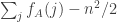 is at most
  . Writing this out, we have
 ,
, .
. , it follows that with high probability
 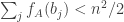 , which implies that
  , then with high probability
  and
and  are of order
  is somewhat like a random walk that is constrained to start and end at zero. There are results that show that random walks have a positive probability of never deviating very far from the origin — at most half a standard deviation, say — so something like the following idea for proving the first step (remaining agnostic for the time being about the precise definition of “close”). We choose some fixed positive integer
  be integers evenly spread through the interval
  . Then we argue — and this should be very straightforward — that with probability bounded away from zero, the values of
  and
and  are close to each other, where here I mean that the difference is at most some small (but fixed) fraction of a standard deviation.
 and
and  are short, that
  and
and  are uniformly close with positive probability.
 and
and  are almost certainly close too. Thomas Budzinski sketches an argument of the first kind, and my guess is that that is indeed needed. But either way, I think it ought to be possible to prove something like this.
 independently (according to some distribution) and conditioning on some suitable event. (A quick thought here is that it would be enough if we could approximate the distribution of
  is the marginal distribution of that
 ![[n]](https://s0.wp.com/latex.php?latex=%5Bn%5D&bg=ffffff&fg=333333&s=0&c=20201002) and subsets of
and subsets of ![[2n-1]](https://s0.wp.com/latex.php?latex=%5B2n-1%5D&bg=ffffff&fg=333333&s=0&c=20201002) of size
of size  one takes the subset
  , and given a subset
 ![S=\{s_1,\dots,s_n\}\subset[2n-1]](https://s0.wp.com/latex.php?latex=S%3D%5C%7Bs_1%2C%5Cdots%2Cs_n%5C%7D%5Csubset%5B2n-1%5D&bg=ffffff&fg=333333&s=0&c=20201002) , where the
, where the  are written in increasing order, one takes the multiset of all values
  , with multiplicity.) Somehow a subset of
  and conditioning on the number of elements being exactly
  , chosen uniformly from all such sequences. A die
  if the number of pairs
  such that
  exceeds the number of pairs
  . If the two numbers are the same, we say that
  and
and  .
. mod
mod  , and arrows into
  . It is not hard to check that the probability that there is an arrow from
  and
and ![A=(a_1,\dots,a_n)\in[n]^n](https://s0.wp.com/latex.php?latex=A%3D%28a_1%2C%5Cdots%2Ca_n%29%5Cin%5Bn%5D%5En&bg=ffffff&fg=333333&s=0&c=20201002) we define a function
we define a function ![f_A:[n]\to[n]](https://s0.wp.com/latex.php?latex=f_A%3A%5Bn%5D%5Cto%5Bn%5D&bg=ffffff&fg=333333&s=0&c=20201002) by setting
by setting  plus half the number of
  . We also define
  to be
to be  . It is not hard to verify that
  , ties with
  , and loses to
  .
. . What is the probability that
  by
by  . We can then ask it as follows. Suppose we choose a sequence
  of
of  , where the terms of the sequence are independent and uniformly distributed. For each
  . What is the probability that
  given that
  ?
? , where the
  are i.i.d. random variables taking values in
  (at least if
  , it ought to be the case that if we sum up the probabilities that
  over positive
  of size comparable to the standard deviation. It will not tell you the probability of belonging to some subset of the y-axis (even for discrete random variables). Another problem is that the central limit on its own does not give information about the rate of convergence to a Gaussian, whereas here we require one.
 when
when  converges very well after
  . To prove this the steps were as follows.
 is at most
  (for some
  is at least
  for some absolute constant
  .
. for every
  to be
to be
 is shorthand for
  ,
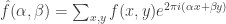
, ![f(x,y)=\mathbb P[(U,V)=(x,y)]](https://s0.wp.com/latex.php?latex=f%28x%2Cy%29%3D%5Cmathbb+P%5B%28U%2CV%29%3D%28x%2Cy%29%5D&bg=ffffff&fg=333333&s=0&c=20201002) , and
, and  .
. not to be too close to 1. But for now I want to concentrate on how one proves a statement like this, since that is perhaps the least standard part of the argument.
 to be very close to 1. This condition basically tells us that
  is highly concentrated mod 1: indeed, if
  takes approximately the same value almost all the time, so the average is roughly equal to that value, which has modulus 1; conversely, if
  are reasonably spread about.
  , let
, let  , and consider the values of
  and
and  . Then a typical order of magnitude of
  is around
  , and one can prove without too much trouble (here the Berry-Esseen theorem was helpful to keep the proof short) that the probability that
 and applying the above argument in each interval. (While writing this I’m coming to think that I could just as easily have gone for progressions of length 3, not that it matters much.) Then in each interval there is a reasonable probability of getting the above inequality to hold many times, from which one can prove that with very high probability it holds many times.
  is of order 1, which gives that the values
  are far from constant whenever the above inequality holds. So by averaging we end up with a good upper bound for
  , then the above argument doesn’t work, because we can’t choose
  , the logarithmic factor being there because we need to operate in many different intervals in order to get the probability to be high. We will get many quadruples where
 of order
  , basically because
  has order
  for small
  is bounded above by a large negative power of
  (since
  is about
  ), so we are in good shape provided that
  .
. of the events hold is exponentially small in
  . A simpler argument of a similar flavour shows that
  is smaller than this and
  .
. (which are independent and each have characteristic function
  ) is
) is  . And then the inversion formula tells us that
![\mathbb P[(\sum_iU_i,\sum_iV_i)=(x,y)]=\int_{(\alpha,\beta)\in\mathbb T^2}\hat f(\alpha,\beta)^ne(-\alpha x-\beta y)\mathop{d\alpha}\mathop{d\beta}](https://s0.wp.com/latex.php?latex=%5Cmathbb+P%5B%28%5Csum_iU_i%2C%5Csum_iV_i%29%3D%28x%2Cy%29%5D%3D%5Cint_%7B%28%5Calpha%2C%5Cbeta%29%5Cin%5Cmathbb+T%5E2%7D%5Chat+f%28%5Calpha%2C%5Cbeta%29%5Ene%28-%5Calpha+x-%5Cbeta+y%29%5Cmathop%7Bd%5Calpha%7D%5Cmathop%7Bd%5Cbeta%7D&bg=ffffff&fg=333333&s=0&c=20201002)
 that lie outside a small rectangle (of width
  in the
  in the
  and the bound on
  ,
, this is
  . It therefore follows from the two-dimensional version of Taylor’s theorem that
 that can be bounded above by a constant times
  .
. for
for  we have that
  , and provided
  is small enough,
  is well approximated by
  .
.  is very well approximated, at least when
  .
. .)
.) be a random variable on
  for
for ![\mathbb P[(X,Y)=(x,y)]](https://s0.wp.com/latex.php?latex=%5Cmathbb+P%5B%28X%2CY%29%3D%28x%2Cy%29%5D&bg=ffffff&fg=333333&s=0&c=20201002) . If we take
. If we take  is
is
 .
. , but I’ll sometimes think of them as belonging to
  too.
too. and the inversion formula
 are
are 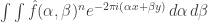 .
. by an expression of the form
  for some suitable quadratic form in
  , and then, since Fourier transforms (and inverse Fourier transforms) take Gaussians to Gaussians, when we invert this one, we should get a Gaussian-type formula for
  and
and  is supported in a small region around 0, then this turns out not to be too much of a problem.
 times with respect to
  .
. . Also, for every
  . This allows us to get a very good handle on the Taylor expansion of

 is the partial derivative operator with respect to the first coordinate,
  the mixed partial derivative, and so on.
 ,
,  , and
, and  .
.  ,
, , which in turn is at most
  .
.  (where
  .
.  as well. For any particular
 ![A=(a_1,\dots,a_n)\in [n]^n](https://s0.wp.com/latex.php?latex=A%3D%28a_1%2C%5Cdots%2Ca_n%29%5Cin+%5Bn%5D%5En&bg=ffffff&fg=333333&s=0&c=20201002) , the probability that
, the probability that  is bounded above by
  for an absolute constant
  ) is at most
  , and in particular is small when
  . I think that with a bit more effort we could probably prove that
  is at most
  , which would allow us to improve the bound for the error term, but I think we can afford the logarithmic factor here, so I won’t worry about this. So we get an error of
  .
. . So for our error to be small, we want
  and
and  .
.  is bounded away from 1 by significantly more than
  and
and  .
. and let us split up the sum into pairs of terms with
  , for
, for  . So each pair of terms will take the form
 .
. , then the modulus of the sum of the two terms is at most
  .
.  are mostly reasonably well distributed in an interval between
  and
and  , as seems very likely to be the case. Then the ratios above vary in a range from about
  to
to  . But that should imply that the entire sum, when divided by
  . (This analysis obviously isn’t correct when
  , since the modulus can’t be negative, but once we’re in that regime, then it really is easy to establish the bounds we want.)
 , then this gives us
  , and raising that to the power
  , which is tiny.
  not to be tiny we need
  are all small but the numbers
  vary quite a bit, so a similar argument can be used to show that in this case too the Fourier transform is not close enough to 1 for its
  are reasonably uniform in a range of width around
  sums and they lie in a rectangle of area
  . Loosely speaking, the information that
 ![[n]=\{1,2,\dots,n\}](https://s0.wp.com/latex.php?latex=%5Bn%5D%3D%5C%7B1%2C2%2C%5Cdots%2Cn%5C%7D&bg=ffffff&fg=333333&s=0&c=20201002) such that
such that  , which is of course the average value of a random element of
 are three vertices chosen independently at random in this graph, then the probability that
  is a directed cycle is what you expect for a random tournament, namely 1/8.
 beats
beats  beats
beats 
 , all the
  possibilities for which
  have probability approximately
  . This would imply, for example, that if
  beats
beats  given that
  is still
  for the out-degree of a vertex
  for the in-degree. Then let us count the number of ordered triples
  such that
  . Any directed triangle
  in the tournament will give rise to three such triples, namely
  and
and  . And any other triangle will give rise to just one: for example, if
  and
and  we get just the triple
  and
and  plus twice the number of directed triangles. Note that
  .
.  . If almost all in-degrees and almost all out-degrees are roughly
  , then this is approximately
  , which means that the number of directed triangles is approximately
  . That is, in this case, the probability that three dice form an intransitive triple is approximately 1/4, as we are hoping from the conjecture. If on the other hand several in-degrees fail to be roughly
  define
  and define
  . Then
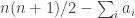
 ![\sum_jg_A(j)=\sum_j\sum_i\mathbf 1_{[a_i\leq j]}=\sum_i(n-a_i+1)](https://s0.wp.com/latex.php?latex=%5Csum_jg_A%28j%29%3D%5Csum_j%5Csum_i%5Cmathbf+1_%7B%5Ba_i%5Cleq+j%5D%7D%3D%5Csum_i%28n-a_i%2B1%29&bg=ffffff&fg=333333&s=0&c=20201002)
 ,
, .
.![\sum_jh_A(b_j)=\sum_j(\sum_i\mathbf 1_{a_i\leq b_j}-b_j)=\sum_{i,j}\mathbf 1_{[a_i\leq b_j]}-n(n+1)/2.](https://s0.wp.com/latex.php?latex=%5Csum_jh_A%28b_j%29%3D%5Csum_j%28%5Csum_i%5Cmathbf+1_%7Ba_i%5Cleq+b_j%7D-b_j%29%3D%5Csum_%7Bi%2Cj%7D%5Cmathbf+1_%7B%5Ba_i%5Cleq+b_j%5D%7D-n%28n%2B1%29%2F2.&bg=ffffff&fg=333333&s=0&c=20201002)
 sufficiently infrequently to make no real difference to what is going on (which is not problematic, as a slightly more complicated but still fairly simple function can be used instead of
  is positive.
![\mathbb P\Bigl[\sum_jh_A(b_j)>0\Bigm|\sum_jb_j=n(n+1)/2\Bigr]\approx 1/2](https://s0.wp.com/latex.php?latex=%5Cmathbb+P%5CBigl%5B%5Csum_jh_A%28b_j%29%3E0%5CBigm%7C%5Csum_jb_j%3Dn%28n%2B1%29%2F2%5CBigr%5D%5Capprox+1%2F2&bg=ffffff&fg=333333&s=0&c=20201002) .
.
 , where
  .
. have mean zero). But a bivariate normal distribution is centrally symmetric, so we expect the distribution of
 ![[X|Y=0]](https://s0.wp.com/latex.php?latex=%5BX%7CY%3D0%5D&bg=ffffff&fg=333333&s=0&c=20201002) to be approximately centrally symmetric, which would imply what we wanted above, since that is equivalent to the statement that
to be approximately centrally symmetric, which would imply what we wanted above, since that is equivalent to the statement that ![\mathbb P[X>0|Y=0]\approx 1/2](https://s0.wp.com/latex.php?latex=%5Cmathbb+P%5BX%3E0%7CY%3D0%5D%5Capprox+1%2F2&bg=ffffff&fg=333333&s=0&c=20201002) .
. ![[X\geq x\wedge Y\geq y]](https://s0.wp.com/latex.php?latex=%5BX%5Cgeq+x%5Cwedge+Y%5Cgeq+y%5D&bg=ffffff&fg=333333&s=0&c=20201002) but not of a “probability zero” event such as
but not of a “probability zero” event such as ![[X>0\wedge Y=0]](https://s0.wp.com/latex.php?latex=%5BX%3E0%5Cwedge+Y%3D0%5D&bg=ffffff&fg=333333&s=0&c=20201002) .
. . (I’m not 100% sure I’ve got that right: the theorem in question is Theorem 2.1.1 from
  — then one will have to add together an extremely large number of copies of
 ![[n] - (n+1)/2](https://s0.wp.com/latex.php?latex=%5Bn%5D+-+%28n%2B1%29%2F2&bg=ffffff&fg=333333&s=0&c=20201002) . (In particular, if
. (In particular, if ![[-(n-1)/2, (n-1)/2]](https://s0.wp.com/latex.php?latex=%5B-%28n-1%29%2F2%2C+%28n-1%29%2F2%5D&bg=ffffff&fg=333333&s=0&c=20201002) .)
.) ![(a_1,\dots,a_n)\in[n]^n](https://s0.wp.com/latex.php?latex=%28a_1%2C%5Cdots%2Ca_n%29%5Cin%5Bn%5D%5En&bg=ffffff&fg=333333&s=0&c=20201002) , then the expected number of
, then the expected number of  is
is  , by standard probabilistic estimates, so if we set
  , then this is at most
  , which we can make a lot smaller than
  . (I think
  and
and  at least somewhere. I’ll sketch a proof of this. Let
  and let
  be evenly spaced in
  is around
  , so the probability that it is less than
  . The same is true of the conditional probability that
  is less than
  (the worst case being when this value is 0). So the probability that this happens for every
  . This is much smaller than
  in magnitude at least
  is at least
  and
and  . Then as
  and the values taken by
  . For this example, all the points
  live in the lattice of points
  such that
  is a multiple of 5.
  and
and  and
and  given that
 ![j\in[n]](https://s0.wp.com/latex.php?latex=j%5Cin%5Bn%5D&bg=ffffff&fg=333333&s=0&c=20201002) , I define
, I define ![\sum_i\mathbf 1_{[a_i\leq j]}-j](https://s0.wp.com/latex.php?latex=%5Csum_i%5Cmathbf+1_%7B%5Ba_i%5Cleq+j%5D%7D-j&bg=ffffff&fg=333333&s=0&c=20201002) . Therefore, if
. Therefore, if  is another die, or even just an arbitrary sequence in
 ![\sum_jh_A(c_j)=\sum_j(\sum_i\mathbf 1_{[a_i\leq c_j]}-c_j)=\sum_{i,j}\mathbf 1_{[a_i\leq c_j]} - \sum_jc_j](https://s0.wp.com/latex.php?latex=%5Csum_jh_A%28c_j%29%3D%5Csum_j%28%5Csum_i%5Cmathbf+1_%7B%5Ba_i%5Cleq+c_j%5D%7D-c_j%29%3D%5Csum_%7Bi%2Cj%7D%5Cmathbf+1_%7B%5Ba_i%5Cleq+c_j%5D%7D+-+%5Csum_jc_j&bg=ffffff&fg=333333&s=0&c=20201002) .
. and no
  and
and  ? I expect the answer to this question to be the same as the answer to the original transitivity question, but I haven’t checked as carefully as I should that my cavalier approach to ties isn’t problematic.
 .
. are zero, which for random
  being zero, we will get something that approximates a bivariate normal distribution. Although that may not be completely straightforward to prove rigorously, tools such as the Berry-Esseen theorem ought to be helpful, and I’d be surprised if this was impossibly hard. But for now I’m aiming at a heuristic argument, so I want simply to assume it.
 and
and  are typically quite strongly correlated. (There are good reasons to expect this to be the case, and I’ve tested it computationally too.) Also, we expect correlations between these variables and
  and
and  that are not independent, and understand precisely the circumstances that guarantee that
  is determined by the matrix of correlations. Let this matrix be split up as
  , where
  is the
  covariance matrix of
  is a
is a  matrix,
  is a
is a  matrix and
  is the matrix
  . A general result about conditioning joint normal distributions on a subset of the variables tells us, if I understand the result correctly, that the covariance matrix of
  . (I got this
  then the covariance matrix of
 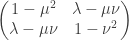 .
. I would have ended up with
  .
. to equal
  . That is, we want
![[-1,1]](https://s0.wp.com/latex.php?latex=%5B-1%2C1%5D&bg=ffffff&fg=333333&s=0&c=20201002) , so any mistakes there might have been didn’t jump out at me. I might just rewrite the code from scratch without looking at the old version.)
, so any mistakes there might have been didn’t jump out at me. I might just rewrite the code from scratch without looking at the old version.) , then you are not completely wrong. The formula for the vector triple product is
 .
. . Now this is the scalar triple product of the three vectors
  , and
, and  to be orthogonal to
  . A nicer way of thinking of it (because more symmetrical) is that we want the orthogonal projections of
  ,
, .
. ,
,  and
and  really do appear to satisfy the relationship
  .corr
.corr corr
corr![\sum_{i,j}\mathbf 1_{[a_i>b_j]}>\sum_{i,j}\mathbf 1_{[a_i<b_j]}.](https://s0.wp.com/latex.php?latex=%5Csum_%7Bi%2Cj%7D%5Cmathbf+1_%7B%5Ba_i%3Eb_j%5D%7D%3E%5Csum_%7Bi%2Cj%7D%5Cmathbf+1_%7B%5Ba_i%3Cb_j%5D%7D.&bg=ffffff&fg=333333&s=0&c=20201002)
 and
and ![f_A(j)=\sum_i(\mathbf 1_{[a_i>j]}-\mathbf 1_{[a_i<j]})=|\{i:a_i>j\}|-|\{i:a_i<j\}|.](https://s0.wp.com/latex.php?latex=f_A%28j%29%3D%5Csum_i%28%5Cmathbf+1_%7B%5Ba_i%3Ej%5D%7D-%5Cmathbf+1_%7B%5Ba_i%3Cj%5D%7D%29%3D%7C%5C%7Bi%3Aa_i%3Ej%5C%7D%7C-%7C%5C%7Bi%3Aa_i%3Cj%5C%7D%7C.&bg=ffffff&fg=333333&s=0&c=20201002)
 , which is equivalent to the statement that
  .
. for roughly half of all dice
  for roughly half of all dice
 ![\sum_jf_A(j)=\sum_{i,j}(\mathbf 1_{[a_i>j]}-\mathbf 1_{[a_i<j]})](https://s0.wp.com/latex.php?latex=%5Csum_jf_A%28j%29%3D%5Csum_%7Bi%2Cj%7D%28%5Cmathbf+1_%7B%5Ba_i%3Ej%5D%7D-%5Cmathbf+1_%7B%5Ba_i%3Cj%5D%7D%29&bg=ffffff&fg=333333&s=0&c=20201002)

 .
. and
and  which would normally be approximately equal to
  .
. . I would therefore like to get a picture of what a typical sequence
  looks like. I’m pretty sure that
  and
and  correlate, since this will help us get some idea of the variance of
  , or similar quantities anyway, but I don’t want to walk before I can fly.
 is always equal to
  , and that is true if and only if
  is uniformly distributed. (The distributions of the
  that will surely make it easier for the global average to be
  .
. are chosen independently and uniformly from
  given that the average of the
 ). We also know that the probability that
  . So the variance of the sum of the
  , so the standard deviation is proportional to
  is roughly constant for
  .
. , then
  are approximately independent. (Of course, this would apply to any
  of the
  , together with the probability that
 ![[j]](https://s0.wp.com/latex.php?latex=%5Bj%5D&bg=ffffff&fg=333333&s=0&c=20201002) and
and  that are uniform on
  and we want to know how likely it is that they add up to
  , the sum of the
  and
and  , and the sum of the rest. So we end up with a double sum of products of three probabilities at the end instead of a single sum of products of two probabilities. The reason I haven’t done this is that I am quite busy with other things and the calculation will need a strong stomach. I’d be very happy if someone else did it. But if not, I will attempt it at some point over the next … well, I don’t want to commit myself too strongly, but perhaps the next week or two. At this stage I’m just interested in the heuristic approach — assume that probabilities one knows are roughly normal are in fact given by an exact formula of the form
  .
. , should that be helpful). Under what conditions can we be confident that the sum
  , which if
 ![\mathbb P[\sum_jg_A(c_j)=n(n+1)/2+t|\sum_jc_j=n(n+1)/2]](https://s0.wp.com/latex.php?latex=%5Cmathbb+P%5B%5Csum_jg_A%28c_j%29%3Dn%28n%2B1%29%2F2%2Bt%7C%5Csum_jc_j%3Dn%28n%2B1%29%2F2%5D&bg=ffffff&fg=333333&s=0&c=20201002) , where now the
, where now the ![\mathbb P[X|Y]](https://s0.wp.com/latex.php?latex=%5Cmathbb+P%5BX%7CY%5D&bg=ffffff&fg=333333&s=0&c=20201002) , we find that it’s going to be fairly easy to estimate the probabilities of
, we find that it’s going to be fairly easy to estimate the probabilities of ![\mathbb P[Y|X]](https://s0.wp.com/latex.php?latex=%5Cmathbb+P%5BY%7CX%5D&bg=ffffff&fg=333333&s=0&c=20201002) than it is to calculate
than it is to calculate ![\mathbb P[X\wedge Y]](https://s0.wp.com/latex.php?latex=%5Cmathbb+P%5BX%5Cwedge+Y%5D&bg=ffffff&fg=333333&s=0&c=20201002) . From that all else should follow. And I think that what we’d like is a nice condition on
. From that all else should follow. And I think that what we’d like is a nice condition on