Posting a LaTeX manuscript on arxiv is straightforward.
Compile your document (say, main.tex). It is okay to leave all your figures in a "figs/" subfolder. Unlike some outlets, you don't have to flatten your directory structure.
Apart from main.tex, main.bbl [bibliography], and figures, you may delete all other files. You need the bbl file because arxiv does not run bibtex.
Zip the folder, and upload on arxiv.
If you have a supplementary information document (say, si.tex) and you use the "xr" package to cross-reference between main.tex and si.tex, then a few extra steps are required. arxiv compiles all tex files in the zipped folder in alphabetic order. So it is important that "main.tex" appears before "si.tex", in case your tex files have different labels.
Compile main.tex and si.tex several times on your machine, so that inter-document cross-references work as desired.
Apart from main.tex, si.tex, main.bbl, si.bbl, main.aux, si.aux, and figures, you may delete all other files. [xr uses main.aux and si.aux.]
Relabel main.tex to main_ren.tex, main.bbl to main_ren.bbl, si.tex to si_ren.tex, and si.bbl to si_ren.bbl. Do not relabel *.aux files. Do not compile.
Vector graphics (SVG/PDF) outputs of scatterplots with thousands of points lead to bloated files, unlike say raster formats like PNG. This makes scrolling PDF documents that include such bloated files a painful affair. The reason is fairly obvious: vector files scale with the number of data-points, while raster files scale with the number of pixels.
There are many potential solutions. The simplest is to rasterize only the large dataset of scatter points using the rasterized=True flag. Thus, plt.plot(x, y, 'o', alpha=0.1, rasterized=True) The resulting PDF is much lighter.
Suppose you want to merge two bib files (f1.bib and f2.bib) that have considerable overlap. One easy solution using Jabref works as described below.
Suppose the target bibliography file without duplicates is merge.bib.
1. Copy f1.bib to merge.bib [cp f1.bib merge.bib]
2. Open merge.bib with Jabref
3. Then click File > Import into current database and select the other file [f2.bib]
4. You get a dialog box which allows you to manually decide what entries/versions you want to retain. If both f1.bib and f2.bib are of comparable quality, you can select "Deselect all duplicates" which automatically unselects duplicated entries.
5. Hit "OK" and save the modfied database [Ctrl-S]
latexify is a Python package to compile a fragment of Python source code to a corresponding expression.
2. Pylustrator Pylustrator offers an interactive interface to find the best way to present your data in a figure for publication. Added formatting an styling can be saved by automatically generated code. To compose multiple figures to panels, pylustrator can compose different subfigures to a single figure. See Youtube demo.
Often I have a document in LaTeX, and somebody else needs an editable copy in Word. Here is a list of hacks I have learnt to use:
1. If the document is relatively free of math and figures then the simplest course is often to compile a PDF, and "import" the PDF into MS Word. This works out remarkably well in many cases.
2. The same thing above applies to figures. You can now directly drop PDF images into a Word doc.
3. If you have lots of equations, then it is worthwhile to use pandoc
4. Many journals accept PDF figures. If they need TIFF, then you can use Adobe Acrobat online to do this conversion. In my experience, this produces smaller files compared to other automatic converters including ImageMagick.
Often, I have a big folder like Lectures/ which may have sub-folders based on topics, and each topic might have additional folders. To clean auxillary LaTeX files in one fell swoop use,
Christopher Bishop has an excellent set (1, 2, and 3) of introductory lectures on "Probabilistic Graphical Models". They are well-motivated and cover topics that include:
directed and undirected graphs
conditional independence
factor graphs
inference using factor graphs and sum/product rules
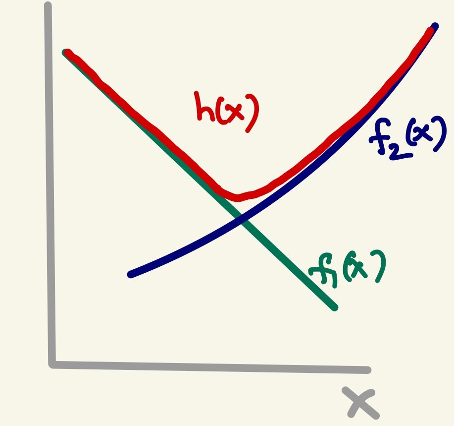
Stitching together two functions is sometimes required as a way to transition from one dependence to another. The following schematic describes the idea pictorially:
Two different approaches are considered in this PDF (or this Jupyter Notebook).
Consider the problem described in this StackOverFlow post. You have a function with certain smoothness properties that are apparent on a log-log plot. This is often accompanied by a large domain of integration. It seems worthwhile to "integrate in logspace", whatever that means. This Jupyter notebook probes this question and makes some recommendations.
Suppose part of a python file uses spaces for indentation, while another part uses tabs. This will throw up exceptions at runtime. So the question is how to fix it.
One answer is to use the python script reindent.py. Stick it in some folder (~/bin/) in the default path and make it executable (chmod +x reindent.py).
Problem: I have a manuscript TeX file (main.tex), and an independent supporting information file (si.tex). I was to cross-reference (using \label and \ref) items across the two files.
For example, I might want to reference figure 1 from si.tex in main.tex.
Solution: As this SO answer suggests, the answer lies in the CTAN package xr.
In main.tex, just include "si.tex" as an external documents, and all its labels become visible!
Say you want to fit a line to (x,y) data. With polyfit, you can say,
coeff = np.polyfit(x, y, 1)
With numpy 1.7 and greater, you can also request the estimated covariance matrix,
coeff, cov = np.polyfit(x, y, 1, cov=True)
The standard error on the parameters is the square-root of the diagonal elements
print(np.sqrt(np.diag(cov)))
This report referenced in the SO page is quite useful!
It hits the key points of what makes multinormal distributions special (conditionals and marginals are normal too!), and the visuals help build intuition.
You might not need this, but I like this essay because it is jargon-free, and focuses on how to get things going. There is python code at the end, which you can play with.
This "bible" is astonishingly well-written. If you are familiar with linear algebra and some statistics, this is a breezy read. Plus, all the important formulae and algorithms you see in different articles, are available here in one place!
I use Preview (on my Mac laptop) and Foxit Reader (on my Linux Desktop) to read PDFs.
While reading papers, I often find myself clicking on links to citations. This takes me to the reference section. After looking up the citation, I like to go back to the previous location on the paper (right before clicking on the link).
How to go back to the "previous view" isn't well documented.
In Preview, the short cut is "Cmd + [" and "Cmd + ]".
In Foxit Reader for Linux (v2.4 and above) the short cut is "Alt + Left Arrow" and "Alt + Right Arrow", respectively.
Matplotlib (v2 and higher) uses "mathtext" to render math by default. It is quite capable, but I don't like the default font, and prefer the classic "Computer Modern" font.
You can fix this globally by modifying the rc file in your custom-style file (use the command matplotlib.get_configdir() to find location) by adding the line:
mathtext.fontset : cm
If you want to render all text using LaTeX (this slows down rendering somewhat), then use: