Kaetemi

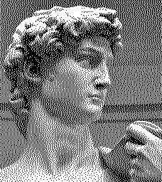
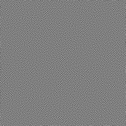
The finest blue noise in the galaxy.

In short, alternate per-pixel between Floyd-Steinberg and Jarvis-Judice-Ninke error diffusion kernels using the lowbias32 randomizer function.

Background on dithering techniques and blue noise

The purpose of dithering is to allow quantizing analog or higher precision data into lower bit depth while minimizing loss of information, aliasing, banding, or other artifacts. Techniques used for this generally fall under either using an ordered dithering mask (e.g. Bayer, void-and-cluster, etc.) or forms of error diffusion (Floyd-Steinberg, sigma-delta, etc.) Similarly to resampling kernels, dithering kernels for 2D processing are distinct from 1D kernels, as the signal distribution becomes spatial rather than purely linear. These techniques are relevant both for quantizing to low bit depths (e.g. printing, e-ink, embedded hardware, etc.), as well as for quantizing high-precision authored content into common file formats (e.g. floating point to 8-bit/channel).

Ordered dithering

Ordered dithering is implemented by using a pre-calculated threshold mask to decide whether to round up or down. The threshold mask is usually an 8-bit bitmap.

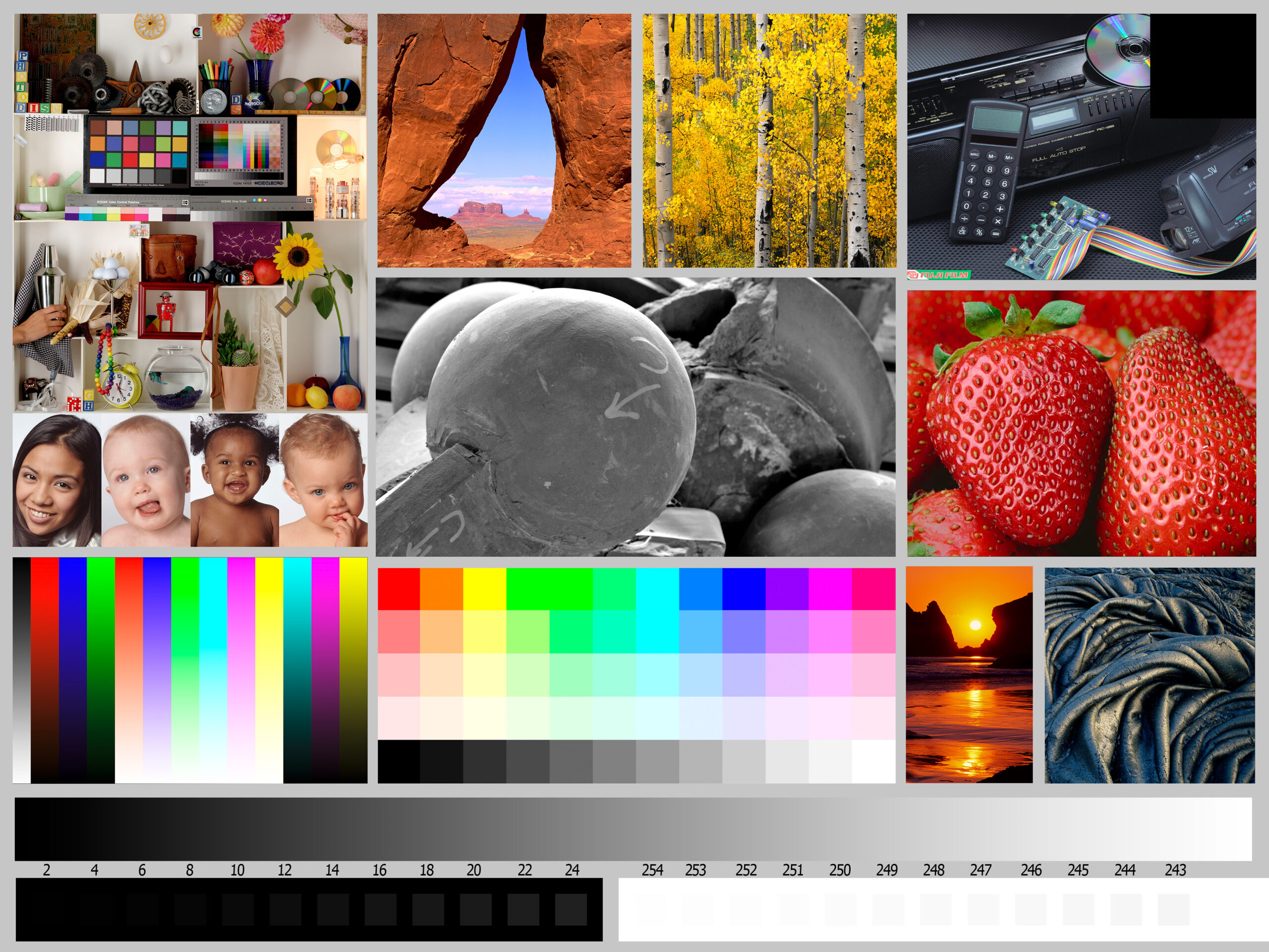
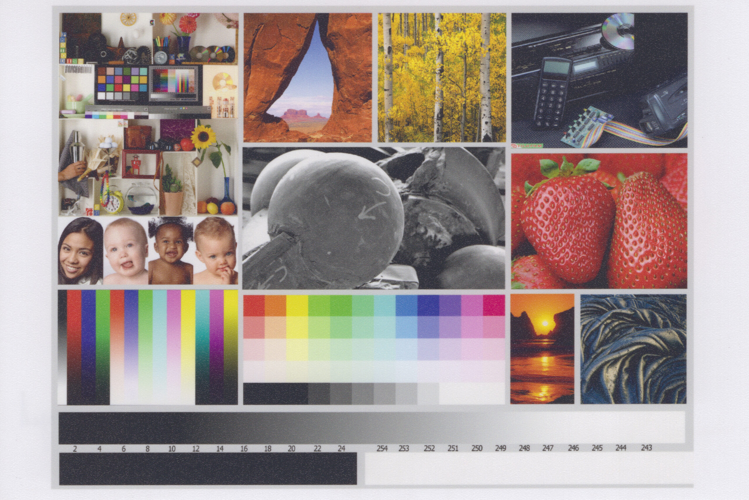
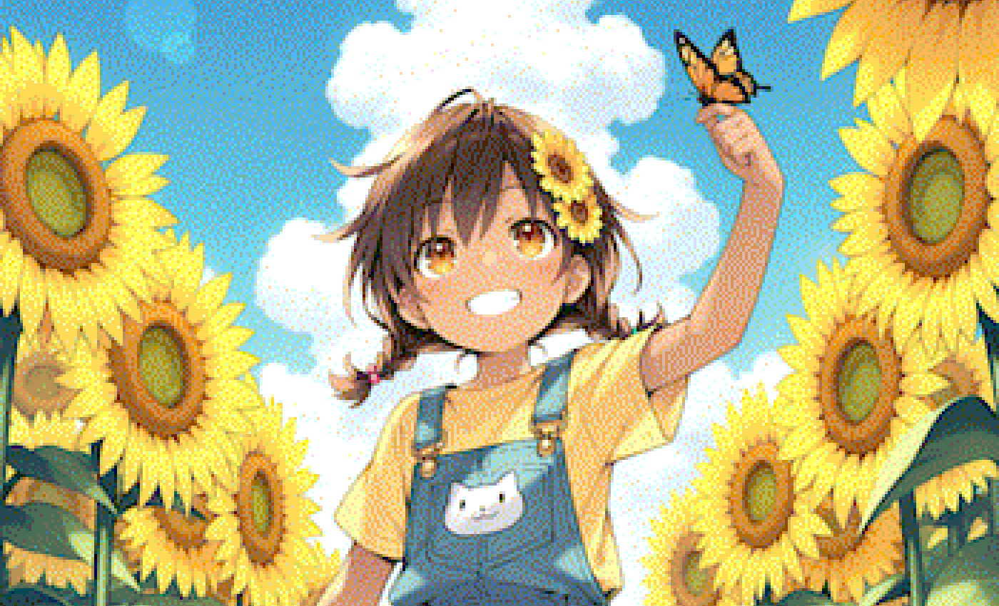
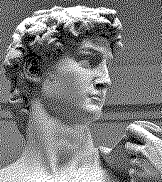
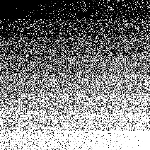
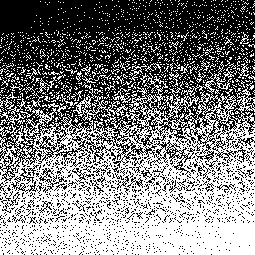
(Make sure your browser is displaying the images at 1:1 display pixel size to ensure proper comparison.)

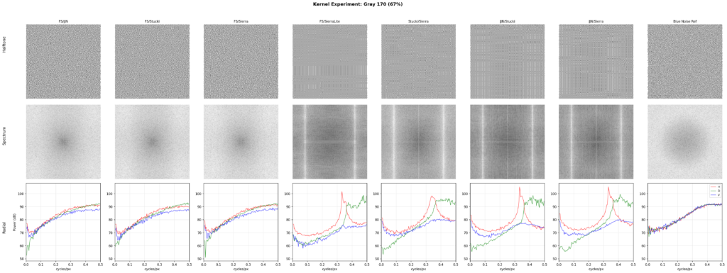
Error diffusion dithering

Floyd-Steinberg and Jarvis-Judice-Ninke kernels are the two earliest 2D error diffusion kernels described in literature. Several variants exist which make adjustments purely for hardware performance reasons, but which don’t offer any quality benefits, so I will skip over these. One problem with the FS kernel are strongly noticeable patterns at certain gray levels. The JJN kernel does not suffer this problem as much, but is larger and looks much coarser, while at the same time slightly sharpening the image features.

Error diffusion is implemented by selecting the color nearest to the target color, and carrying over the remainder error to neighboring pixels. The target color is modified by adding the carried over error before quantization. A kernel, which is just a small table of numbers, describes what fraction of the error each of the neighboring pixels receive.

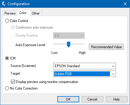
Color space awareness

For color space-aware dithering, the color distance can be calculated in a perceptual color space (e.g. Oklab Lr), and the error must be accumulated in a linear color space (e.g. linear RGB). These can be distinct from the actual quantized color space (e.g. sRGB).

Conventionally, dithering test images are processed without color space conversion, treating the input as linear. We follow this convention for the 1-bit comparisons to enable direct comparison with reference literature. For multi-channel or higher bit depth outputs we apply proper color space conversion.

Perturbation and blue noise

In 1988, Ulichney demonstrated perturbed variants of Floyd-Steinberg dithering, in particular a 30% randomization of the threshold, and a random 50% alternation between pairs within the kernel, effectively randomly switching between 4 modified variants of the Floyd-Steinberg kernel. This technique breaks up the patterns of the kernel by introducing a tiny amount of white noise. The resulting spectrum of reference gray levels was described as strongly suppressing low frequencies, with the error diffused evenly into high frequencies, and called blue noise. These techniques as described by Ulichney were not optimized as described, but demonstrate the principle and the concept of blue noise, and viable paths in improving dithering quality.

A spectrum analysis of these techniques shows a first-order blue noise curve approaching a ~6dB power density per octave, similar to the spectrum of a 1D sigma-delta ADC with TPDF (effectively, also threshold perturbation) as used in audio engineering.

To imagine blue noise, it can be explained as the more intuitive (yet fallacious) version of a coin flip, where after several heads you’re more likely to get a tails, the gambler’s false sense of fairness, or in other words, random numbers with a negative autocorrelation.

Stochastic kernel-switching (our method)

Our method is a specific variant of kernel weight perturbation, which simply switches between the proven FS and JJN kernels, using the high bits of the lowbias32 hash function as randomizer. This technique is simple and unambiguous to implement, is fast, has near-perfect blue noise characteristics, eliminates pattern formation entirely, introduces less white noise than alternatives, and can be applied also to multi-level as well as non-uniform quantization.

Weight perturbation methods

Existing weight perturbation methods compared here include Ostromoukhov, which switches between 128 pre-calculated kernels depending on the gray level, and Zhou-Fang, which extends Ostromoukhov with positional modulation. The Ostromoukhov technique attempts to optimize an ideal kernel at every gray level to more closely approach a blue noise profile, however, this limits the practical application of this technique to quantizing from 8-bit to 1-bit, or other uniform power-of-2 ratios that match, and excludes non-uniform colorspace-aware dithering. A failure mode with Ostromoukhov is that flat gray levels in themselves are not perturbed and show patterns. Zhou-Fang expands on this technique with a new pre-calculated table along with a modulation table to further perturb the process based on the pixel position, however, this retains the same applicability limitations.

Ordered blue noise

At present, the most common blue noise derived technique in dithering is using a pre-calculated ordered blue noise threshold mask, such as one generated through the void-and-cluster method. This is as cheap to implement as a Bayer matrix, and highly practical for parallel processing. However, rather than diffusing error, this technique merely masks the error using an approximation of blue noise, reducing the actual signal quality.

Technical comparison

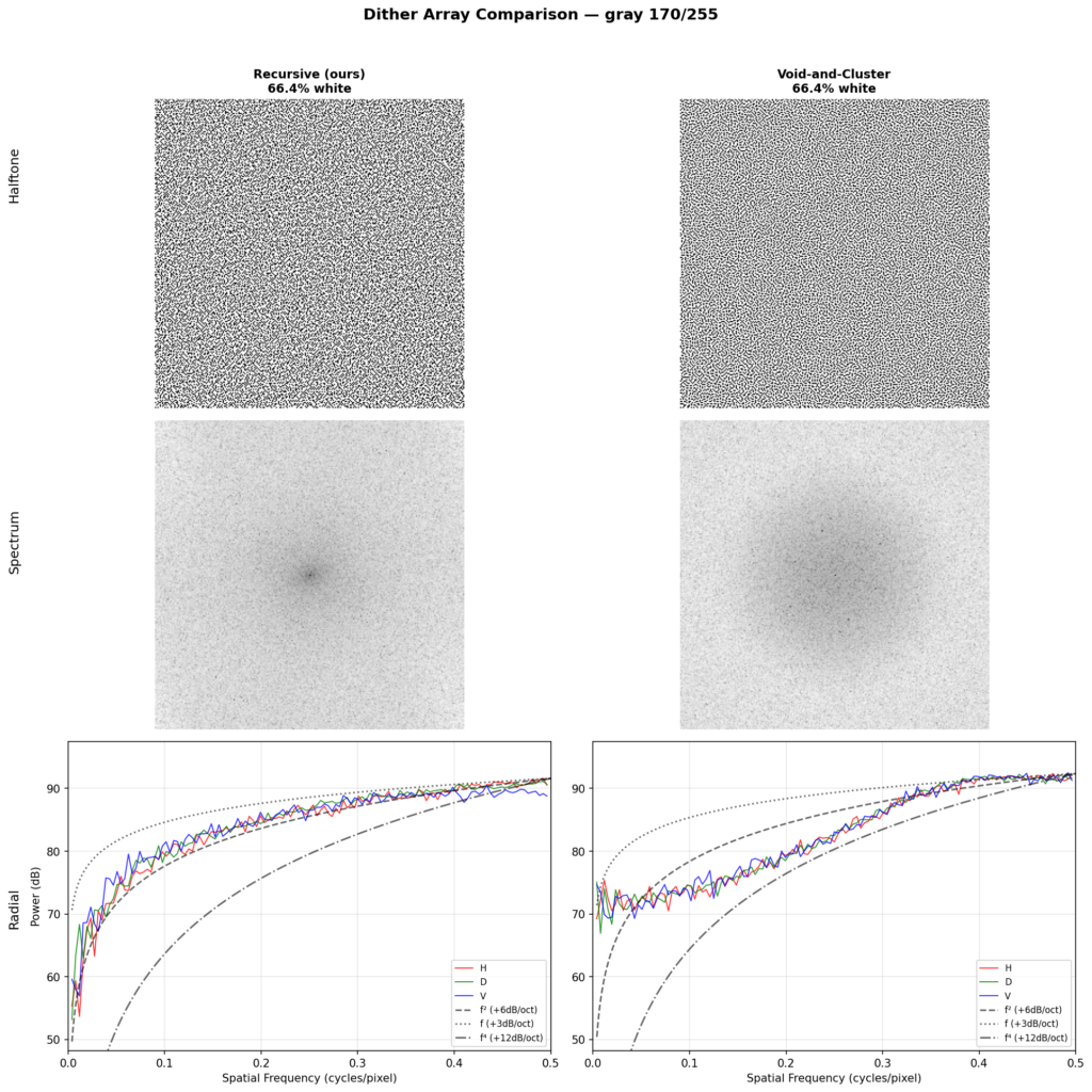
The common objective metric found in literature to compare error diffusion methods is to analyze the spectrum at various levels of gray. This reveals whether the diffusion is in fact blue noise, and the level of isotropy exhibited by it. To read the chart, basically, if the three lines (the horizontal, diagonal, and vertical analysis) align closely together, you have high isotropy. Then, the first part of the chart should just go as low as possible, and the final part of the chart should be a flat peak. The x axis shows spatial frequency from low to high, and the y axis shows power in dB. Isotropy in the lower frequencies is more crucial than in the higher frequencies, as the lower frequencies are more visible. Sharp peaks in the graph show up when patterns form.

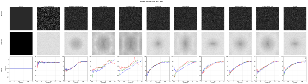
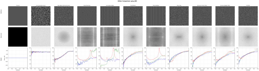
By this metric, our method nearly perfectly aligns with the theoretical ~6dB/octave blue noise curve. The methods described by Ulichney, as well as a variant of Floyd-Steinberg using TPDF for threshold perturbation, similarly approach the same curve. Ostromoukhov’s technique improves on FS, but does not fully eliminate patterns at single gray levels. Zhou-Fang is relatively clean, but the technique vertically introduces some level of noise in the lower ranges due to the modulation being position dependent.

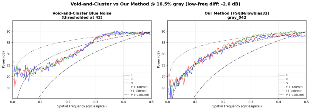
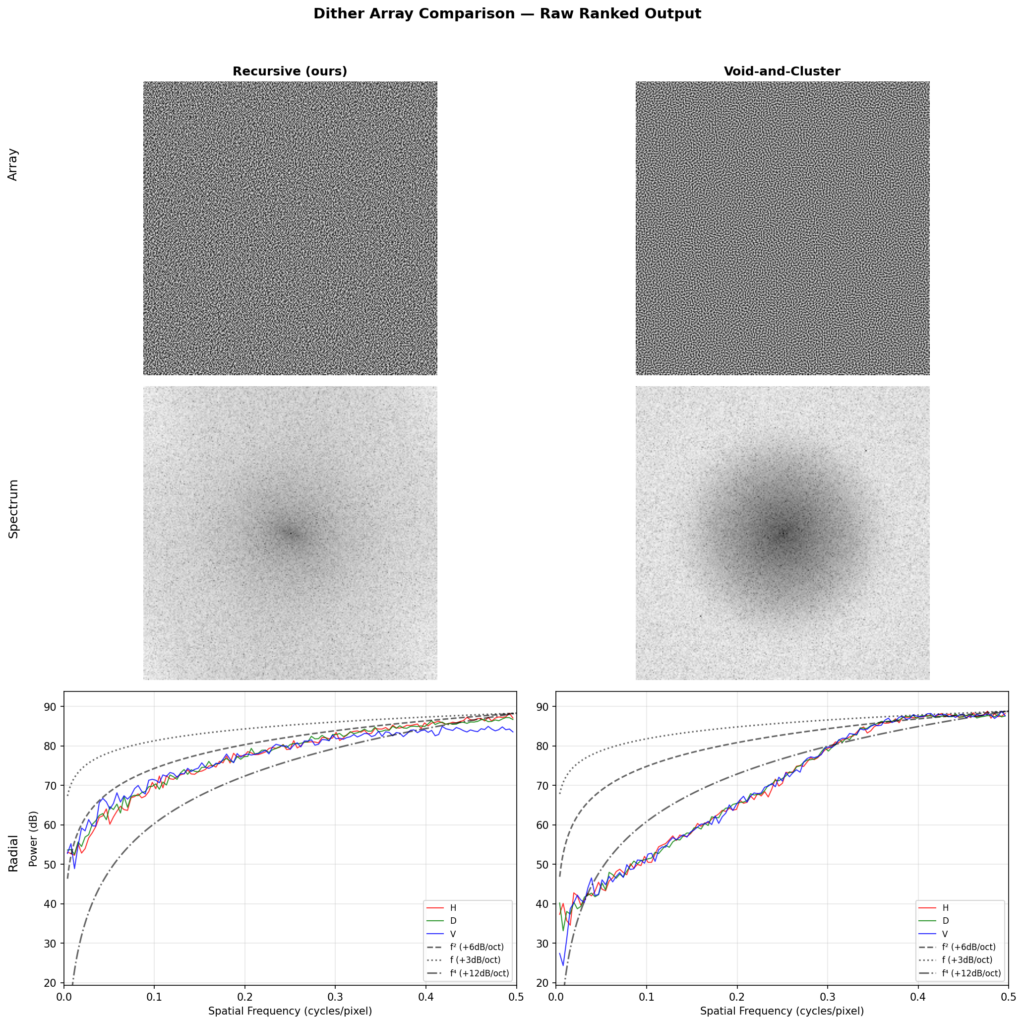
A comparison with theoretical blue noise curves shows our method maintains a consistent 6dB/oct slope across the full frequency range, whereas void-and-cluster (a well-known blue noise approximation) exhibits a steeper rolloff in the midrange that flattens at the extremes.

Ramps and steps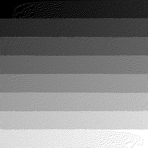

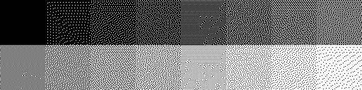
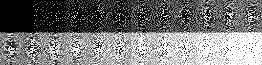
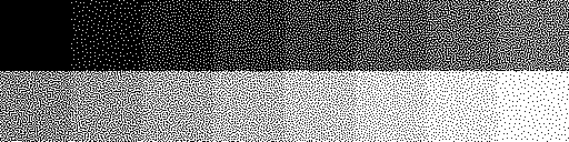
Reference test images

As there are no widely adopted objective metrics in literature for real images, we’re using an approach where the original and quantized image are analyzed in wavelet form, as wavelets happen to model error patterns quite well, and several metrics are then derived from the difference between the original and quantized output at multiple subbands. The resulting set of informal metrics is useful for relatively comparing several desirable aspects between techniques.

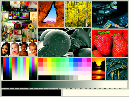
The measurements here are an average made from the following standard images: cameraman, lake, lena_gray_512, livingroom, mandril_gray, pirate, walkbridge, and woman_blonde. The complete test outputs can be found on GitHub.

MethodBluenessFlatnessStructureIsotropyFloyd-Steinberg+0.330.5200.3290.480Floyd-Steinberg (Serpentine)+0.320.5240.3210.484Ulichney (Weight Pertb., Serp.)+0.310.5280.3150.518Ulichney (Threshold Ptb., Serp.)+0.310.5340.3000.549Our method+0.290.5430.3260.578Our method (Serpentine)+0.290.5420.3140.567Ostromoukhov (Serpentine)+0.290.5110.3030.409Floyd-Steinberg (TPDF, Serp.)+0.270.5440.2610.639Zhou-Fang (Serpentine)+0.260.5420.2640.678Jarvis-Judice-Ninke (Serp.)+0.250.5340.3470.569Jarvis-Judice-Ninke+0.240.5320.3600.584Void-and-cluster (Ordered)+0.230.4110.2540.687White noise (Random)+0.000.5620.1970.967None (Banding)-0.420.5010.5780.382

The blueness metric measures how locally the error is getting diffused. A higher score means the error stays close to where it originated rather than spreading into visible large-scale patterns. It’s calculated by comparing the energy level of coarser bands against the finer bands. Floyd-Steinberg as expected has the most local diffusion, as it’s designed to be the smallest possible kernel. JJN, given its size, ranks much coarser. Our method sits right in-between. For comparative purposes, void-and-cluster scores low (even though it is an excellent blue noise approximation) because it doesn’t diffuse the error, it just masks.

Flatness is measured by how flat the spectrum of the error at each band is. A lower score here means there are repetitive error artifact patterns in the output. White noise scores highest in this metric, as it has no patterns. Our method and Zhou-Fang rank at the same level for this metric. Ostromoukhov ranks low here since it exhibits a lot of patterns.

Structure measures how faithfully the halftone output preserves the edges and details of the original image, calculated as a correlation between original and output wavelet coefficients across scales. This score is particularly hurt by noise or blurring smoothness getting added into the target signal. Specifically, threshold-perturbed techniques score poorly on this metric, and techniques which inherently sharpen the image score more highly. Our method scores similarly to FS and JJN. Zhou-Fang ranks low as its position-dependent modulation causes white noise along the vertical axis.

The isotropy shows how consistent the vertical, horizontal, and diagonal errors are, comparatively. Techniques with a higher base noise level do score more highly on this metric by default, so (just as with the other metrics) it needs to be read in relation to the blueness and other metrics, and cannot be considered by itself.

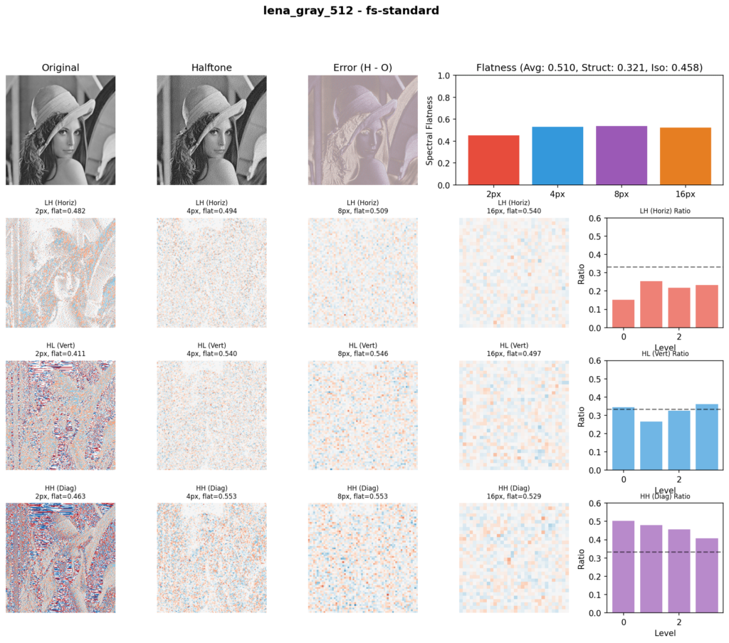
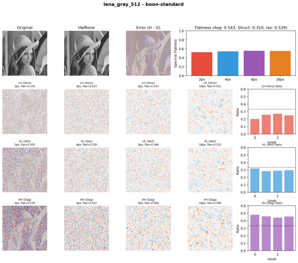
Using these metrics we can get a reasonable objective measure of different techniques. The error patterns clearly highlight themselves in the wavelet analysis. Our method strikes a competitive balance across all four metrics.

Alternative hash pairings

Comparing outputs with various randomizer functions shows minimal practical difference, although the differences are measurable. Our choice here is lowbias32 for its simplicity and cleanest noise profile. Additionally, it is important to prefer the high bits over the low bits, as these have better statistical properties due to better mixing.

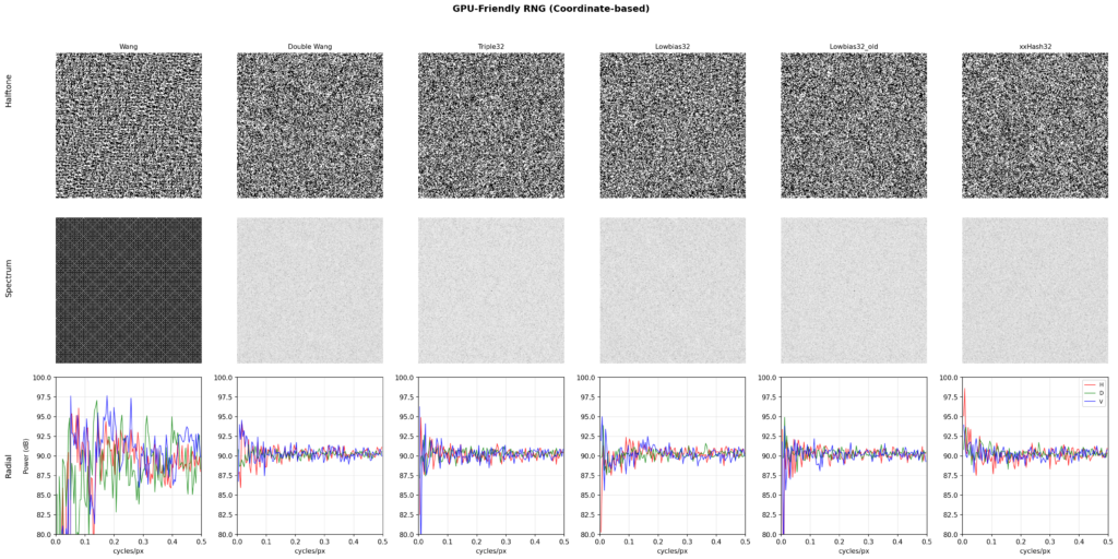
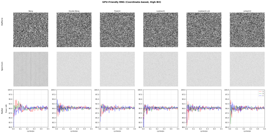
Comparison of coordinate-based pseudo-random number generators, highest (most significant) bit

Wang hash, even with its repetitive behavior when used in a 2D context, still performs adequately when compared to lowbias32, so in practice the choice of randomizer is flexible.

Alternative kernel pairings

Several popular kernels pair well with Floyd-Steinberg. JJN pairs best with FS based on comparisons across gray levels. Pairings between kernels other than FS, however, do not work as well. It seems plausible that at least one of the kernels should be the smallest reliable kernel, and that there exists a more ideal pairing than the one presented here.

Miscellaneous notes

This diffusion technique is easy to implement in existing error diffusion pipelines and has a nearly ideal blue noise profile without diffusion pattern artifacts.

The random seed used for switching kernels can be changed per-frame, this allows the technique to be used for display scanout where the diffusion must temporally vary between frames. Ideally, a 3D kernel may provide more optimal temporal properties for such use cases.

Error diffusion is inherently a stateful serial process, so not straightforward to use in stateless parallel processing contexts, however it is possible to pipeline and process multiple lines simultaneously maintaining a few pixels delay between each line, by synchronizing available work between threads with atomic counters.

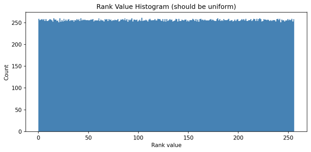
Generative ordered blue noise mapping

It is possible to generate an ordered blue noise map using error dithering as a source, by generating a halftone output for 0.5 gray, and then recursively splitting each low and high population with a new gray halftone, masking out the portions that are not part of the current population (simply setting them at 0 or 1) so the error propagates over them. This population splitting technique is repeated until we have assigned all 256 populations.

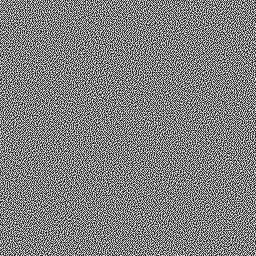
The resulting ordered blue noise has a perfectly uniform distribution, and reasonably maintains its spectral profile accross thresholds. It is plausible that a more ideal kernel pairing may maintain a more consistent spectral profile for this generative task.

Practical applications of 2D error diffusion

• Quantizing ML image generation outputs from FP16 or FP32 to 8-bit/channel PNG
• Low bit depth image formats for embedded hardware
• Display scanout (e-ink, embedded, etc.)
• Printers
• Deterministic generative blue noise maps for procedural placement of foliage in games
• Spatial distribution for stochastic image sampling in rendering techniques

Application in 1D

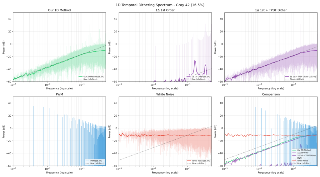
The same technique can be used for 1D quantization, as an alternative to sigma-delta with threshold perturbation dithering. Reasonable kernel pairs are found at [ 1 ] and [ 19, 5 ], [ 1 ] / [ 23, 1 ], and [ 1 ] / [ 7, 5 ] (derived from the 2D JJN kernel). This can likely be further optimized. Performance appears competitive against sigma-delta with dither, and shows less distortion at the lowest threshold ranges.

For the task of producing full-range 1D blue noise using the generative population splitting technique, we found that [ 1 ] and [ 0, 1 ] are ideal kernels. This may also offer some hint towards a more ideal 2D pairing.

Practical applications in 1D

• LED dimming without flicker or strobing interference
• Audio ADC
• LLM token sampling (using generative blue noise)

Example outputs

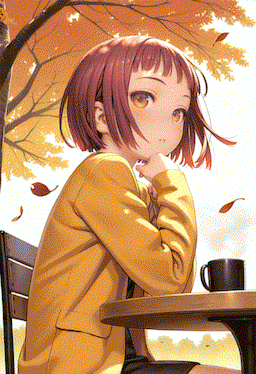
Samples created using the dithering web demo included in the CRA tool. Color space-aware dithering. Ensure you are viewing these at 1:1 pixel size, as browser scaling interpolates in display gamma space which darkens colors at high contrast edges.

In an ideal world, if you scan a photo and then print it, you could expect it to look the same. Of course, that’s not the case with consumer hardware. What’s on the screen, printed, and scanned, never quite matches up. But, there’s no reason for it to be impossible! The only real physical limit is the whiteness of your paper, and the darkness of your ink.

Color spaces are in fact very well defined. A specific color value is by definition always and forever going to be exactly that same color, given the same lighting conditions.

Just to ease any doubts, without delay here’s my final calibration result:

Source image in the top-left, the printed photo below, and a scan of the printed photo on the right.

All you need to reasonably calibrate a printer is a scanner. However, your calibration will only be as good as your scanner’s factory calibration. (Calibrating the scanner yourself is possible too, of course, but may not be necessary for acceptable results.) At the very least you need to be able to disable all automatic adjustments in the scanner software, and specify the scanner’s color space. And the scan should honor those color spaces. The sRGB or Adobe RGB targets are what you should be looking for.

On an EPSON Perfection v39, a budget scanner, it will look something like this:

• 

• 

If your scanner model has a decent reputation, and your scanned image looks color correct, then you should be good. Make sure to set your monitor to sRGB or any appropriate calibration to ensure a good comparison. A monitor with a good reputation regarding its factory calibration is nice to have as well.

For comparison, here’s a book cover scanned at 1200dpi (the JPG is downscaled here) using a multi-function Brother DCP-T500W on the left, and using an EPSON Perfection v39 on the right. The Brother is also the printer which I’m calibrating, and I’m not that inclined to accept its scans as correct, for several reasons.

• 

• 

The lighter colors in the Brother scan are much too saturated and brightened. Skin tones tend to bright yellow, blues are going cyan, and the bright red icon is washed out. This scanner actually does not seem to specify any color space. In the EPSON scan on the right, the colors and contrast closely match the reality of the book cover in front of me. What I see on my screen (which also claims to be sRGB) matches with what’s scanned, so I’m inclined to believe that my monitor and scanner both have a reasonable factory calibration. It matches my expectations. And that’s all what’s needed. A scanner that can promise to scan in a requested color space, and delivers what it’s asked. Automatic enhancements are useless here, they are unpredictable. If I can calibrate my prints to the EPSON scanner, at the very least the prints will also match my expectations.

Important to note, white paper isn’t white. White paper is white-paper color, which is darker than monitor white (which is D65 white). Most regular paper will be slightly blueish (to make it look whiter, and also tends to look like whichever color of light you happen shine at it). Office scanners, such as the Brother multi-function may brighten up scans to make generic paper white match monitor white. This is handy for documents, this is not good for photos or calibration purposes.

Here’s a sample image, along with a scan, printed on the default best quality photo settings (both in sRGB color space here, printed on the Brother, scanned on the EPSON):

• 

• 

It looks a bit dull.

The details, all light colors and black colors, are fully reproduced, but the contrast is rather low, and some of the colors are off. This is not because scans are dull. You may be tempted to “correct” and “enhance” scans, but this scan isn’t actually wrong. The white of a display is simply brighter by definition that the white of paper, and similarly, a display’s black is deeper than the black of printer ink. Your prints should simply not be using the unprintable color space, and that’s where good photo editing can really make a world of difference.

Clearly the printer’s factory settings are stretching the input contrast into the printable range. It’s definitely a very safe and well-designed calibration for easy out-of-the-box printing — unedited photos with bad lighting will print quite well. Dark and light details won’t get lost. Evidently, the defaults here don’t attempt to accurately reproduce the actual color space as it’s defined, but we can change that.

My first attempt at getting better output was to simply let Photoshop manage the color space, and print in CMYK using the FOGRA39 profile using absolute colorimetric mode (after comparing several other standard CMYK profiles.)

The result feels like it’s already a milestone ahead of the factory calibration. Strawberries are edible again. Contrast looks great. Light and dark extremes are clipped off, as expected however. Unfortunately this profile failed on several photos with extreme blue and black colors — dark blue turned darker than black, and saturation varied wildly.

I printed a chart with manual CMYK values. Based on the scan, the cyan mismatches with FOGRA39 standard cyan, measuring a bit too magenta. The magenta and yellow are on point. I created a custom CMYK profile in Photoshop, based on the following chart, which visibly improved the color spectrum.

However, darker blacks now went completely haywire. Then I noticed that the color-mixed CMY black sample on the bottom-left of the chart looked a bit too much like the real black ink sample on top of the chart. I manually printed the color layers to produce the bottom-right sample.

Very different. And also a much deeper black.

Turns out most common inkjet printers only accept RGB data, converting that to CMYK space internally. Any CMYK content that’s printed is converted into RGB by the driver software, before being converted back into CMYK by the printer. So whatever gets sent as CMY black gets turned into plain black (or however the printer wants to print black).

I printed another challenging photo using the FOGRA39 profile again, this time separating all the color layers manually, and sure enough the blacks and blues came out as expected. But the saturation still didn’t look quite right yet. And printing four layers manually is quite a hassle, taking a really long time as well.

Searching for a software solution to generate RGB inkjet printer color profiles, I finally came across Argyll, which supports scanner-based calibration (but also doesn’t recommend doing it). It’s actually a large set of command line tools, so it requires reading a lot of manual pages to figure out how all the pieces that are needed work together.

Here’s what I did.

After a few attempts at calibrating on plain paper, I ended up with the following command line options which gave a reasonable result. I only used this to obtain a first reference calibration, not for printing.

targen -d2 -G -e32 -B32 -s16 -g16 -m8 -f2028 -p0.5 bro_best_3
printtarg -s -t600 -pA4R -iSS bro_best_3
scanin -c "calibrate_077.tif" bro_best_3_01.cht "AdobeRGB1998.icc" bro_best_3
scanin -ca "calibrate_078.tif" bro_best_3_02.cht "AdobeRGB1998.icc" bro_best_3
colprof -v -D"Brother Plain Best" -cmt -dpp -S "AdobeRGB1998.icc" -qh -Za -ta -Ta -r3 bro_best_3

The targen command creates a list of colors that will be printed, printtarg creates the actual files that you need to print.

Very important. You must turn off color management both under Photoshop and under your printer’s drivers. For Brother, you uncheck “Match Monitor” in the advanced options (it will say “Colour Mode: Off” in the main settings screen after you do this). Make sure your remaining print settings exactly match the print settings you want to calibrate for.

Scan the calibration sheets to Adobe RGB or sRGB. The scanin tool turns the scans into a list of measured colors. Finally, the colprof utility is what generates the actual color profile.

Using the cctiff tool, you can create the RGB image that will be sent to the printer, which you can also use to preview your color ranges.

cctiff -ia "PrinterEvaluationImage_V002_Adobe.tif" -ia "bro_best_3.icm" "PrinterEvaluationImage_V002_Adobe.tif" "PrinterEvaluationImage_V002_Adobe_bro_best_3.tif"

The image below shows the output of the plain paper color profile, that is, the raw RGB values which will be sent to the printer. The colors will look weird (usually over-contrasted and -saturated), this is expected.

The whites are clearly compensating strongly for the paper’s blueish shade here. (You can probably calibrate prints for actual colored paper too.) Blacks are heavily clipped, because this is just a light plain paper print. That’s all fine and expected. The only issue in this calibration are the jumps in the gradients, which are caused by not having enough of the right data points (or by a low quality measurement). However, for the purpose of a first reference calibration, this is a good start. I won’t be using this profile to actually print.

A few warnings here. First. The color management in Photoshop will give different behaviour for out-of-range whites and blacks when printing than Argyll’s cctiff tool with these printing profiles. The quality of Argyll’s cctiff tool is much more accurate. You can directly print the output of cctiff using Photoshop with color management disabled, in the same way that the calibration sheets were printed. Second. Using an input file in ProPhoto color space causes an overcompensation on the white point, it will not look as expected. It’s a camera color space with brighter whites. Converting those images to Adobe RGB in absolute color space, before converting to your printer’s profile, works to get exactly what’s on your screen. (Open your ProPhoto file, convert it to Adobe RGB in absolute mode, save as TIFF, use cctiff to create the TIFF in printer color space, and print that with color management disabled.) Either Adobe RGB or sRGB input files will give the same result, but Adobe RGB has a wider input range for saturated colors, so should be preferred for scanning and print preparation if it’s available. Use sRGB for images intended for computer display.

After a bit of fiddling with the settings of the calibration sheets, I ended up with the following command options for calibrating the actual photo paper. The number steps for the grayscale gradient have been increased, additional samples for the outer boundaries of the color space have been added, and three sheets are printed instead of the previous two.

targen -d2 -G -e32 -B32 -s32 -g32 -m8 -f3042 -p0.75 -c bro_best_3s.icm -n32 bro_photo
printtarg -s -t600 -pA4R -iSS bro_photo
scanin -c "calibrate_084.tif" bro_photo_01.cht "AdobeRGB1998.icc" bro_photo
scanin -ca "calibrate_085.tif" bro_photo_02.cht "AdobeRGB1998.icc" bro_photo
scanin -ca "calibrate_086.tif" bro_photo_03.cht "AdobeRGB1998.icc" bro_photo
colprof -v -D"Brother Photo Best" -cmt -dpp -S AdobeRGB1998.icc -qh -Za -ta -Ta -r3 bro_photo

The commands now also include a reference to the previous calibration, allowing the samples to be spread more evenly within the color space, and also adding the neutral white gradient that was previously calibrated.

After running this calibration, and testing the new color profile, I ran the calibration a final time. To further enhance the scale of neutral grays, the new color space is now referenced. The same command options are used for this final calibration, except after the scanin step, the new samples are merged with the previous samples, giving the color profile much more data to work with.

targen -d2 -G -e32 -B32 -s32 -g32 -m8 -f3042 -p0.75 -c "bro_photo.icm" -n32 bro_photo_v2
printtarg -s -t600 -pA4R -iSS bro_photo_v2
scanin -c "calibrate_092.tif" bro_photo_v2_01.cht "AdobeRGB1998.icc" bro_photo_v2
scanin -ca "calibrate_093.tif" bro_photo_v2_02.cht "AdobeRGB1998.icc" bro_photo_v2
scanin -ca "calibrate_094.tif" bro_photo_v2_03.cht "AdobeRGB1998.icc" bro_photo_v2
average -m bro_photo.ti3 bro_photo_v2.ti3 bro_photo_merged.ti3
colprof -v -D"Brother Photo Best (v2 Merged)" -cmt -dpp -S AdobeRGB1998.icc -qh -Za -ta -Ta -r3 bro_photo_merged

Here’s what the calibrated print looks like.

• 

• 

• 

• 

The color space is an excellent match. Unfortunately, the blacks are getting crushed on this printer, giving the prints a magazine look, rather than looking like a real developed photograph. There does not seem to be any option in its driver to increase the ink density. (If you do have the option, try it, and calibrate the photo paper prints again from the start.) To get around this problem, I simply printed over my previous 6 calibration sheets a second time, renaming the previous calibration and running just the scanin, average, and colprof steps again.

Using this new color profile, the output of cctiff, as seen on the screen and after a single print pass, appears much brighter with more contrast range in the dark colors. This is as expected, since the ink will be doubled during the print. The downside of this trick is a reduced sharpness, since the prints are not always perfectly aligned.

The resulting test print looks excellent. From left to right — original file, default photo print settings, photo paper calibration, and the 2-pass photo paper calibration.

• 

• 

• 

• 

After printing twice over on the same sheet of photo paper, using this specially calibrated profile, I can obtain much deeper blacks, without affecting the rest of the color space. The print looks almost like an actual developed photograph, and immensely better than the default settings, so I’m quite happy with this result.

• 

• 

The support team at Brother has given the following response on the blackness of this printer:

Upon consulting with our Technical Team, blank ink will not mix to CMY inks because for DCP-T500W, BK  is classified as pigment, CMY is classified as dye. Our latest models are using dye inks and the method of printing is different. The black ink is now also used in photo printing to produce much vibrant dark images.

Since you cannot install any additional dependencies on function instances, you have to include any missing tools, that you need, as static binaries in your deployment.

To prepare a static build of ImageMagick, which will work on Azure Functions, spin up a Debian 10 x64 VM (the DigitalOcean one works fine), and run the following commands. (Based on the instructions for AWS from https://gist.github.com/bensie/56f51bc33d4a55e2fc9a.)

apt install libpng-dev libjpeg-dev libtiff-dev build-essential
wget https://imagemagick.org/download/ImageMagick-6.9.11-49.zip
unzip ImageMagick-6.9.11-49.zip
cd ImageMagick-6.9.11-49
./configure --prefix=/home/site/wwwroot/imagemagick --enable-shared=no --enable-static=yes
make
make install
tar zcvf ~/imagemagick.tgz /home/site/wwwroot/imagemagick/

Create an imagemagick/bin folder, inside your project, which will be included in the deployment. Download the imagemagick.tgz archive from the VM, and extract just the binaries you need (e.g. convert) into the bin folder. Also include the etc folder as imagemagick/etc. The rest of the files can be ignored.

In your function script, at initialization, use chmod to mark the binaries as executable. For Node.js, this can be done as follows.

const bins = fs.readdirSync('/home/site/wwwroot/imagemagick/bin');
for (let i = 0; i < bins.length; i++) {
    fs.chmodSync('/home/site/wwwroot/imagemagick/bin/' + bins[i], 0o755);
}

For testing purposes, set up a function to output the ImageMagick version information.

const { exec } = require("child_process");
const convert = '/home/site/wwwroot/imagemagick/bin/convert';
module.exports = function (context, req) {
  return exec(convert + ' -version', function (error, stdout, stderr) {
      context.res = {
          body: stdout + '\n' + stderr
      };
      context.done();
  }); 
}

You can use /dev/shm to pass data, between processes, using temporary files in memory (alternatively/tmp for regular disk-backed temporary files), or use stdin and stdout to stream files in and out of the process. Streaming may have more overhead if you have more complex pipelines (when the stream has to pass through your Node.js process). Or you can pipe through multiple commands in one exec call, where practical. Files allow more flexible command line options when combining multiple images, but you need to take care to delete your temporary files.

This is a board I based roughly on a setup we had in high school, that I was taught logic gates with, once upon a time.

I designed the layout about two years ago using Robot Room Copper Connection. Unfortunately, the software has been bought out since, and a full version is no longer available for purchase. (The “new” versions are vendor-locked.)

Recently I ordered some PCB prints along with the prints for another project, and last week I finally put everything together.

The CD4572 chip on the board provides an AND, an OR, and 4 NOT gates. Two of the NOT gates are pre-wired to the AND and OR to get a NAND and NOR, for convenience.

Using this layout, you can teach the basics of logic gates. An AND gate can be constructed using the OR and NOT gates, and an OR gate can be constructed similarly. Once a student is familiar with the logic, they can advance to creating a basic latch (tap a button, and a light stays on), followed by a set-reset latch.

function bradmaxPlayerInit_6a08fc7a9378f() { var bradmaxPlayerConfig_6a08fc7a9378f = {"dataProvider":{"source":[{"url":"https:\/\/cdn.kaetemi.be\/stream\/2020\/logic_board_demo\/logic_board_demo.mpd"}],"splashImages":[{"url":"https:\/\/cdn.kaetemi.be\/stream\/2020\/logic_board_demo\/logic_board_demo.jpg"}]},"mute":true}; var element = document.getElementById("bradmax-player-6a08fc7a9378f"); var player = window.bradmax.player.create(element, bradmaxPlayerConfig_6a08fc7a9378f); // Back compability. if(!window.player) { window.player = player; } } if(window.bradmax && window.bradmax.player) { bradmaxPlayerInit_6a08fc7a9378f(); } else { window.addEventListener('load', bradmaxPlayerInit_6a08fc7a9378f); }

A student can then advance step-by-step to more complex concepts by using subsequent boards which directly provide a set of latches to create a counter. Eventually, learning enough components to build a basic calculator, and moving onto directly using ICs or hardware synthesis languages.

For safety (baby proofing), to avoid shorts, the design puts a resistor in all the wires. (Back in high school, the batteries of the educational boards went bad at suspiciously fast rates.) Output sockets still need to have a diode added in the next revision, since the output status LEDs currently give misleading output when you wire outputs together.

The power supply was constructed from leftover boards of an older revision of another previous project, reusing a portion of the 7805 circuit.

In a next revision, aside from the extra safety diodes on the outputs, adding some convenient buttons to the inputs might be helpful in further lowering the learning curve. A proper solution for the power supply should also be thought of. Additionally, adding some holes in the logic board design for more properly soldering a hard wired supply..

After trying out a USB isolator to fix the audio noise that was caused by a ground loop, I continued my search for a high quality plug-and-play solution to forward audio from my laptop to my desktop.

The solution? Two USB device microcontrollers, bridged by an SPI isolator chip. Two FT932s and an ADuM3151BRSZ. The USB devices will act like an audio output device on one end, and an audio input device on the other. To keep prototyping feasible, I’m using the MM930Mini development module, rather than the bare chip.

Hand soldered at 300°C using a nice big chisel tip. The soldering tutorials on the EEVblog channel are easy to follow.

This board connects the SPI slave from one of the FT930s to the SPI master of the other FT930, through the SPI isolator. The isolator ensures the grounds of both boards remain disconnected from each other. There’s two ports at the edges, which connect directly to the SPI master and slave, for debugging use, and the connectors in-between are wired to the UART TX and RX pins.

The UMFTPD2A board is needed to program the FT930s. It includes a UART channel, which is very useful for debugging. A quick “Hello World” confirms the development boards are in working order.

In order to validate whether the SPI isolator is functioning, I uploaded the “SPI Slave Example 1” and “SPI Master Example 1”, from the FT9xx examples folder, to the development boards. No luck at first though, the data wasn’t coming through.

I changed the example to just test the GPIO function of the pins, toggling them on and off, and log their state through UART, on both sides. Then I measured the pins directly. The SPI master pins were transmitting correctly, the SPI slave pins were receiving correctly, but the SPI slave board was not seeing any incoming data, nor transmitting anything. The SPI isolator did appear to be working correctly, though.

After a bit of searching, I found my problem. While the FT930 does have only one SPI slave device, there are two possible pads to use it. Either pins 34 to 37, or pins 0 to 3. The example was using the former, I designed the wiring on my board to use the latter.

#define GPIO_SPIS_CLK 0
#define GPIO_SPIS_MISO 1
#define GPIO_SPIS_MOSI 2
#define GPIO_SPIS_SS 3

In addition to changing the pin numbers, I also had to change the function that the pins are set to. SPIS is function 2 on the former pad, while it’s function 1 on the latter.

gpio_function(GPIO_SPIS_CLK, pad0_spis0_clk);
gpio_function(GPIO_SPIS_SS, pad3_spis0_ss);
gpio_function(GPIO_SPIS_MOSI, pad2_spis0_mosi);
gpio_function(GPIO_SPIS_MISO, pad1_spis0_miso);

With these adjustments, the example application works as expected. Which validates that the soldered board is functioning as it should. Based on the datasheet of the isolator, the maximum SPI clock rate at 3.3V is 12.5MHz. This aligns well with the FT930 clock of 100MHz, using 8 as the SPI clock divider. The testing example appears to work reliably using this clock speed.

spi_init(SPIM, spi_dir_master, spi_mode_0, 8);

In the next post, I will explore how to set up the FT930 microcontrollers as USB audio devices.

While benchmarking a custom concurrent functor queue against standard library containers, I noticed something that I didn’t expect.

The common concern about the standard containers, especially ones such as std::list, std::map and std::queue, is their poor behaviour in terms of memory allocations. These structures are well known for allocating tons of tiny objects. Frequently, those concerns are downplayed by argumenting that modern memory allocators are well optimized to support these structures. This argument actually seems to hold up, except, until it doesn’t.

My benchmark initially went through different setups of lambdas with 2 large strings in the capture list getting pushed into and popped from different queue containers. One test, sequentially pushing all, and then popping all of 8 million entries. The next doing the same, but on multiple threads. The last test, pushing and popping on multiple threads all at the same time. At first, I didn’t notice anything suspicious. My specialized container was largely outperforming the standard containers. Good for me.

Then, I let the whole set of tests, all being run from a single process, repeat itself 16 times. That’s when something looked way off.

These results were obtained on Windows 10 version 1909, using Visual Studio 2019 version 16.6.5, on an AMD Ryzen 5 2600 with 32GB RAM.

Most of the benchmarks got slower over time! Not just by a little bit. They slowed down by a lot! The ones that were not affected, were the benchmarks which were doing the push and pop operations all concurrently. Or, in other words, the benchmarks that didn’t allocate a lot of memory didn’t noticeably slow down. It was only the benchmarks doing a large amount of memory allocations that slowed down over time.

Could it really be? Standard library containers are really that bad? I ran the single threaded benchmarks for each container separately, to validate my assumption. The testing code is available on GitHub.

While I always assumed STL containers were rather bad for performance critical use, for use in games especially, I couldn’t believe it was really this bad.

My custom container, which allocates memory in larger fixed blocks, and serially writes functor objects into those blocks, was barely affected. The standard containers, which allocate individual objects for each entry that’s added, slowed down dramatically over time in the benchmark.

It obviously appears that the STL containers are causing some heavy memory fragmentation here. Or, at least, causing the memory allocator to break down in performance, at some point, in some way or another.

A couple of days later, I reviewed my benchmark. Actually, the testing code had the new and delete operators replaced by a custom implementation to keep track of the allocation to ensure there are no memory leaks anywhere. Just a simple atomic counter, though. The allocation was implemented using _aligned_malloc and _aligned_free. I removed these custom implementations, and ran the tests again, just to be sure my benchmarks were correct.

Oh, no! After all this time, _aligned_malloc was the culprit? The slowdown just disappeared entirely! I tried putting the custom new and delete operators back in again, this time with regular malloc. The result remained the same. No more slowdown either. Even more, the new benchmarks actually appeared to go faster over time!

Something was clearly off with _aligned_malloc here. Or was there?

I wondered. What if I roll my own aligned allocator on top of malloc? Just pad the size, align the pointer, and store the original pointer. That shouldn’t be much slower than when directly calling malloc…

Uhh. That doesn’t look right. Or, well, maybe it does? Exactly the same result as with _aligned_malloc. What is going on here? It’s nothing more than a slightly larger allocation, isn’t it?

I changed the benchmark to increase the capture list to 3 strings, instead of the original 2 strings, and also reverted back to the malloc implementation which had no slowdown in the previous test.

Slightly larger memory allocations, both causing a massive slowdown over time? It’s even worse than before. What is going on here?

It was time to look deeper. I wrote a simple test to directly benchmark the malloc function. Allocating a large amount of memory with varying small sizes, again repeating the test 16 times, following a FIFO allocation and freeing behaviour to match the queue containers’ behaviour. All of the tests showed huge slowdowns by the last round. But none of them showed good performance, so this gave no indication of what was triggering it.

In a next set of tests, instead of varying the allocation size, I varied the total amount of memory to allocate in each testing cycle.

There it is! The slowdown consistently gets triggered just past the 4GB total allocation mark. But, why? Does this always happen, or are small allocations really the culprit after all? Are large allocations immune, or not?

Repeatedly allocating 2GB and below was showing no problems at all. At just over 4GB the decay slowly started to become noticeable, but once at 8GB the performance dropped like a brick over time.

Using the worst-case total allocation size of 8GB, I varied the allocation sizes again. This time trying out larger allocation sizes, as the tiny allocations from one of the earlier tests all resulted in a similar performance slowdown. The testing code is available in case you want to verify these results.

You might’ve fairly expected that the results would make some sense. The larger allocations of 1MB and above were fast, and didn’t appear to be causing any performance issues over time. And the smallest allocation size tested caused a rather significant slowdown. Makes sense.

Once the test went below 1MB, to 512kB allocations, the slowdown slowly but visibly kicked in. So far, so good.

But here’s the part where it got interesting.

At 256kB, just another drop down to the next lower power-of-2, memory allocations became fast again! Without any sign of performance issues.

How could that be? Going down further to 128kB the performance slowdown appeared yet again, and at 64kB the memory allocations even peaked, getting up to 10 times slower! But, then, going for an even smaller allocation size of 32kB, once more all performance issues were suddenly gone. And once at 16kB and below, where the LFH (low fragmentation heap) kicks in, the slowdown issue came back, but with a different curve, and even earlier.

Where 512kB, 128kB, and especially 64kB sized allocations were causing massive performance slowdowns over time, allocations of 32kB and 256kB remained blazingly fast in comparison. I have found no explanation for these specific values.

In this test, all allocation sizes were clean powers-of-two. According to a presentation on the Windows heap, which I found online, allocations have a header padding of 16 to 32 bytes. I could confirm this behaviour by logging a sequence of allocated addresses.

000002A7C4118B50
000002A7C4120B60
000002A7C4128B70
000002A7C4130B80
000002A7C4138B90
000002A7C4140BA0

What if I’d simply subtract 32 bytes from the power-of-two sizes? The abovementioned presentation document also mentions that remainders of 32 bytes in allocation blocks are not recycled into the heap for smaller allocations, so this appears to be a safe value to use.

That actually worked! No more significant performance slowdowns, except for the 16kB minus 32 bytes allocation.

As mentioned before, allocations of 16kB and lower are handled by the LFH according to its documentation. The performance graph for the 16kB allocations in the previous test was also noticeably different in shape compared to the other graphs, which confirms that this is indeed the case.

I wondered if the allocation sizes which didn’t suffer from this issue would end up getting affected when the slowdown does occur due to other allocations, so I ran another test for this case, alternating between allocating 8GB in blocks of 64kB, and blocks of 64kB minus 32 bytes.

Based on this test, it seems the slowdown that’s caused by problematic allocation sizes does slightly affect the performance of other allocations which normally wouldn’t show this issue. However, the better allocation sizes still did keep showing better performance overall than the worse allocation sizes in all cases.

In short, small allocations below 16kB are actually optimized to be pretty fast. Until they reach over 4GB in total size. Then, performance gets slower and slower over time, even if you free all the allocated memory in your process.

So, don’t allocate more than 4GB of RAM using allocation sizes of 16kB and below, and avoid allocating exactly 64kB, 128kB, or 512kB. Ideally, allocate memory in 1MB or larger memory chunks, or allocate powers-of-two minus 32 bytes (minus 80 bytes in debug mode, due to a 48 bytes additional debug header) for smaller allocation sizes above 16kB. Aligned allocation functions pad your allocation size, which needs to be taken into account. A 64kB allocation size turns out to be the worst performer of all.

Hi, I’m Jan, also known as Kaetemi in the online world. I am working on LibSEv, a simple event loop library with optimized support for C++ lambdas, a clean C interface, and C++ exception safety. Buy me a coffee through Patreon if you’d like to support this project!

I actually happened to be using just that allocation size, 64kB, as the default allocation size in my custom container. After modifying my custom functor queue to allocate 32 bytes less than a power-of-two block, performance was indeed significantly boosted. The test intentionally creates a large amount of std::string instances to ensure that the performance slowdown was in effect in all results in this chart.

Looking further through the documentation on the Windows heap, I came across the HeapCompact function. It appears this function merges empty sequences of fragmented memory together.

Could this be it? I adjusted the test to call HeapCompact(GetProcessHeap(), 0) inbetween each testing round.

Problem fixed. I guess? At least, when it’s called whenever the allocated memory gets below the 4GB marker again. It took only 10 milliseconds to call this function in my tests, too. Perhaps it might be a good idea to call this function occasionally in software projects, whenever possible. For example, it could be called before and after loading screens in a game, or before and after loading a project or document in a productivity application.

It turns out heap fragmentation still is a real issue, and can occur even in unexpected situations. Memory allocation sizes do have a significant effect in solving the associated performance issues. But when staying within certain limitations there is really none-to-little measurable effect of any memory fragmentation that STL containers may or may not be causing, although there still is the fixed overhead of simply making more allocations. Allocators are actually pretty well optimized for this usage. Benchmarks of STL containers can be wildly deceiving.

The following rules-of-thumb seem practical, as tested on Windows 10 version 1909, using Visual Studio 2019 version 16.6.5.

• Don’t allocate more than 2 to 4GB of total memory in small sizes.
• Prefer allocations of 16kB and below for short-lived small size allocations.
• When possible, avoid allocations of 16kB and below, and of exactly 64kB, 128kB, or 512kB.
• If you absolutely need a power-of-two, allocate memory in sizes exactly 32kB, 256kB, or 1MB and up.
• Otherwise, use an allocation size that’s a power-of-two minus 32 bytes (or minus 80 bytes in debug.)
• Call HeapCompact(GetProcessHeap(), 0) before and after voluminous operations.

These results are Windows-specific, and the specific measurements do not apply to other operating systems. However, following the above recommendations should not negatively affect your performance on other operating systems. If in doubt, run your own benchmarks.

If you liked this article, you might also enjoy my 6-part series on reverse engineering the 3ds Max file format. Have fun reading!

A selection of the test results in this article have also been tested and reproduced on an AMD Ryzen 7 3700X with 32GB memory, running Windows 10 version 2004, using Visual Studio 2019 version 16.7.1.

Executables signed with a reputable code signing certificate get better SmartScreen treatment. A signed executable proves that it hasn’t been tampered with by anyone who does not have the signature key.

To sign your code, you’ll need to generate a private key and public certificate. The public certificate will need to be signed by a certificate provider to validate your organization.

This process uses OpenSSL and Windows.

Generate the private key and certificate signing request using the following command.

openssl req -utf8 -nodes -newkey rsa:4096 -keyout NAME.key -out NAME.csr

Enter your details. Submit the contents of the name.csr file to your certificate provider (e.g. Xolphin), ordering a code signing certificate. Organization Validation is the cheapest option, goes around EUR 100 for a year’s validity. Go through the validation process.

The name.key file contains your private key. Your certificate provider will never see this file. Keep it safe.

When ready, you’ll get a collection link in the mail. This will download a file, which might be called CollectCCC, user.crt, or something else, depending on your provider. This file contains your public certificate, signed by the certificate provider. Rename the collected certificate to name.p7s or name.crt, depending on the file type. If you got a zip file instead, and it contains a name.crt file, use that one.

Install the public p7s or crt file to your Personal certificate store. Using the Windows certificate manager. Right click your certificate and export it to the base64 format. Save as name.cer. Delete the public certificate from the certificate manager, since it’s useless.

Issue the following command to combine the signed name.cer certificate with your private key name.key.

openssl pkcs12 -export -out NAME.pfx -inkey NAME.key -in NAME.cer

This creates a name.pfx file, which you can install directly in the Personal certificate store on the computer where you want to sign your executables. You can use the Windows certificate manager to add a friendly name to the certificate.

To sign an executable, run signtool, as follows. Set the timestamp provider appropriately. Both exe as well as dll can be signed. The certificate fingerprint can be found by opening the certificate’s details panel.

"C:\Program Files\Microsoft SDKs\Windows\v6.0A\Bin\signtool.exe" sign /sha1 YOUR_CERTIFICATE_FINGERPRINT /t http://timestamp.comodoca.com/authenticode "helloworld.exe"

Right click your executable, and check Properties, to verify.

A couple of days ago, when hooking up my laptop to my PC’s line input, I was met with an unacceptable noise that I found was coming from a ground loop. Disconnecting the laptop’s own ground indeed solved the issue, but grounding the laptop through the audio cable obviously isn’t ideal.

While looking instead for digital USB to USB solutions, which do not seem to exist on the market, I did come across the ADuM3160, a USB isolator.

What does this do, and why is it important? Very simple. It isolates all the lines of a USB connection, including the power and ground. That immediately solves the ground loop. This image from the manufacturer’s website illustrates it well.

And luckily, there exist a ton of cheap USB isolator modules with this chip. So I got myself one of those to try it out, plus a USB audio adapter for less than €1.

There’s an interesting twist to these off-the-shelf devices. They also add an isolated DC to DC converter into the module, which is what allows them to actually provide power from the host to an attached device, without requiring a separate external power source.

I can confirm that this solution works perfectly. After reconnecting the laptop’s ground, there is absolutely no noise on the audio anymore. Although, the sound quality of the audio adapter isn’t much to write home about…

Perhaps I could isolate the USB audio card of the desktop instead, and then connect the laptop’s internal audio to its line input. That would ground the desktop’s USB audio card through the audio cable to the laptop’s ground instead, which isn’t too bad.

While this works well enough, having to go through analog, especially using the cheap audio adapter, isn’t ideal. Unfortunately, there doesn’t appear to be an off the shelf USB to USB solution, and neither have I found any ICs with a dual USB device controller.

Another approach might be hooking up two FT932s. The FT93x is a USB device controller. But, rather than the USB isolator on one end, using an SPI isolator between them. They’d then have to be programmed to appear as a speaker output on one end, and a line input on the other end. This solution would allow for a plug-and-play digital audio connection between two devices, without requiring any special software configuration.

I’m setting up my old laptop next to my desktop. Currently my desktop, running Windows 10, is connected to an old Creative X-Fi USB sound card that’s no longer supported. It has some wonky drivers, but has pretty clean and crisp sound output when all the enhancement effects are turned off. For now, I can keep using that as long as it works. The laptop is running Linux Mint 19.3, and has a regular stereo jack audio output.

The obvious solution is hooking up the audio output of the laptop to the line in of the PC. Unfortunately, this solution picks up an unusable amount of line noise.

A software solution then, PulseAudio has a Windows build which supposedly can be used as an audio server that the Linux laptop could connect to. Streaming the audio over the network is reasonable. However, the last build for Windows appears to be 7 years old, and way behind the Linux version, so I’m going to pass on that.

How else could I hook this up?

USB to USB. I could pass the audio directly digitally using some device which passes as a USB speaker on one end, and a USB line in on the other end. So far I haven’t found any existing. Fortunately, I may be able to build this with some off-the-shelf components, either USB-I²S-USB or USB-S/PDIF-USB. The second solution has the advantage of having known support for optical isolation, which definitely would avoid any weird business going on. So far, I can’t find any S/PDIF USB input, though, so it might not be feasible.

For the USB to I²S to USB route, the PCM2076 appears to be solving one side of the story. Not sure if there are any out-of-the-box I²S to USB line input solutions, but we could build this ourselves using an FT900 board as a last resort. With some luck, we can optically isolate the I²S signal as well. This seems to be possible at least using an IL715E.

This website with a modular DAC seems to pop up a lot in online search results, so I’ll keep that bookmarked here as a reference.

Another solution could be simply to find or build a sound card with multiple USB inputs, instead of passing the audio through to the PC first.

To be continued.