Vasek Rozhon's blog

We published our video on zero-knowledge proofs!

Surprisingly, making this video took a lot of work. Zero-knowledge proofs for coloring are one of those algorithms that, in hindsight, seem beautifully simple and clean. But that’s just an illusion—there’s actually a lot going on behind the scenes. We struggled with deciding how in-depth to go and which applications to discuss. In the end, the video covers a bit of everything, and I hope different viewers will find something that sparks their curiosity. If that’s the case, you should definitely check out some slower, more in-depth sources; zero-knowledge proofs are realistically too difficult to understand them from 20 minutes of a video. For example, the following book on cryptography is a classic: https://www.wisdom.weizmann.ac.il/~oded/foc.html

Here’s a list of topics that did not make it in the video.

1. How to reduce satisfiability to coloring?

We pointed out that almost everything can be reduced to 3-coloring. This is closely connected to our video on NP-completeness—many problems can be formulated as “here is a (polynomial-time) algorithm checking solutions: can you find an input that is accepted by it?” Such an algorithm can be represented as a circuit, and each circuit can be thought of as a collection of constraints on Boolean variables—that is, the satisfiability problem.

Here’s how you can convert a concrete satisfiability problem into graph coloring with three colors. The image below shows a satisfiability problem asking us to set binary variables to some values so that the formula is satisfied. We assume that each constraint in the problem is a disjunction of a few variables or their negations; any satisfiability problem can be converted into this form. 1 Below the formula is an equivalent graph 3-coloring problem.

And here’s the explanation for the picture:

Explanation of the parts of the graph:

Each part—usually called a gadget—plays a specific role in translating the satisfiability problem into a coloring problem.

Triangle Gadget:

There’s a triangle where each vertex must be colored with one of three colors. In the second picture, I already colored the nodes of the triangle with red, blue, and green. This makes it simpler to talk about the coloring; instead of saying “This node has to have the same color as the top node in the triangle,” we can say “This node has to be green.”

Variable Gadget:

We represent each variable with an edge between two nodes. All these nodes are connected to the green node, which means that in any valid solution, the edge is either colored red-blue or blue-red. This represents whether the variable is true or false.

Clause Gadget:

For a clause like OR OR , we think of it as “the only forbidden combination is .” Our task is to construct a gadget that eliminates this one forbidden combination while allowing all others. Here’s how: if both and are false (represented as the edge being colored red-blue), the node labeled OR must be blue. Similarly, the node labeled OR OR must be blue. You can verify that any other combination is acceptable.

2. My Favorite Theorem

At the end of the video, we mentioned that zero-knowledge proofs address the question “what can be done without a trusted authority?” By “trusted authority,” we mean someone that everybody trusts to be honest and keep their secrets safe—like a bank, a state, or a software company. Zero-knowledge proofs show that we can achieve certain tasks without any trusted authority.

But zero-knowledge proofs are only about tasks of the type “convince others I can do something”. We can be much more ambitious! For example:

• How can we vote without a trusted authority?
  In state elections, we trust the state to count votes honestly while maintaining privacy. But here’s a long-shot hope: Could there be a distributed system that does the same without relying on any trusted authority?
• How can we keep and exchange money without a bank?
  In financial transactions, we trust banks to handle our money honestly while preserving privacy. Again, could a distributed system achieve the same without relying on a bank?

As it turns out, for both questions—and all similar ones—the answer is yes, at least in theory. In the second case, the implementation is, (in)famously, the cryptocurrencies. There are also blockchain protocols that attempt to implement secure private voting.

The fact that all this is possible is supported by one of my favorite theorems from theoretical computer science, proven a few years after the introduction of zero-knowledge proofs. The paper is called How to play ANY mental game, it’s by Goldreich (wrote the book I linked at the beginning), Micali (I had an office pretty close to his when I was at MIT, but sadly never met him there), and Wigderson (Received Turing award recently, his work on cryptography such as this paper was cited as one of the reasons).

Their theorem uses the setup of the Byzantine generals problem (which we covered in an earlier video). In this problem, a group of generals wants to coordinate—in our basic case, each general started with 1 bit of information and they wanted to agree on a common bit. However, the theorem’s setup is more general—each general starts with some information , and together they want to simulate an algorithm that takes inputs and outputs some result . For example, if is a vote-counting algorithm, each represents who the general numbered votes for, and is the elected candidate. We want a distributed simulation of the algorithm such that:

• The input of each general remains private (except for the information leaked by making public).
• This privacy holds even if a some fraction of generals are traitors who try to disrupt the simulation of or extract information from the loyal generals.

For example, if there were a trusted authority—say, a universally trusted queen— among the generals, we could have each general send to her, have her simulate , and then announce . But the theorem by Goldreich, Micali, Wigderson says that the same can be done without any trusted authority, and for any algorithm .

It is perhaps not surprising that zero-knowledge proofs are a crucial component of the proof. The rough idea is to split the simulation of among the generals so that each one performs a computation on data that is meaningless without the context of what the others are doing. For example, a general might be asked to “receive two numbers from generals 8 and 42, sum them, and send the result to general 4.” Using commitment schemes and zero-knowledge proofs, the general can convince others that he performed this computation correctly without revealing the actual numbers. This way, we can keep all the generals to be coordinated in their simulation of , while each is only doing small piece of the overall computation and can’t really say what’s going on globally.

In practice, implementing cryptocurrencies by simply following this theorem would be incredibly inefficient. Nonetheless, the theorem is a powerful theoretical result demonstrating that many tasks can be accomplished without a trusted authority. Moreover, zero-knowledge proofs are used in blockchain practice. For instance, you could use them to implement private transactions. — on typical blockchains, all transactions are public, but with zero-knowledge proofs, you can prove you have enough funds for a transaction without revealing your balance. There are also methods to use zero-knowledge proofs to speed up blockchains by verifying certain requirements off-chain (as far as I can say people are actually more excited by this second application).

Noninteractive Proofs

Our zero-knowledge proof was interactive—a back-and-forth conversation between the prover and the verifier. This approach is not ideal in practice; for example, what if you want to prove the same fact to many people? It would be better if the prover could simply publish a document that everyone can verify. This is called a noninteractive proof, and it is how we typically think of proofs.

One fact that I believe isn’t as well-known as it should be is that the interactivity of our protocol isn’t inherent and can be removed rather easily. Here’s how:

First, imagine there is what’s sometimes called a beacon—a public source of randomness that everyone can observe. For example, you might imagine that a distant star emits light that we measure here on Earth, and we all agree on how to convert the tiny fluctuations in the strength of the signal into a stream of random bits.

In that case, we can “implement” a verifier as follows: we choose random bits emitted by the beacon at some time and use these bits to simulate the random challenges issued by the verifier. In the end, our proof is a transcript of the conversation between the prover and the verifier, along with the time . Any verifier can check that the transcript is valid and that the verifier used the random bits from the beacon at time .

And that’s it—a noninteractive proof. There are some subtle issues, such as the possibility of us trying to cheat by using some specific time for which the stream of random bits has some helpful property. However, the probability of successfully cheating in our protocol for a specific time is extremely low, and we can make it so low that even when considering all possible , the overall chance of us cheating remains negligible.

In practice, you don’t even need a beacon. Instead, if the protocol has rounds, you first commit to your graph times and record all the commits to form a string . Then, you pass through a cryptographic hash function to produce a “random” string , which you use to simulate the verifier. Although the bits in aren’t truly random, they are unpredictable because cryptographic hash functions are one-way, so this is pretty much equivalent to using the truly random beacon. The right terminology for the bits in the string is that they are pseudorandom—yet another topic in one of our recent videos. While working on this video, I really felt that all the topics we covered recently are coming together.

1. We could even assume that each disjunction has three variables—a so-called 3SAT form—but the number of variables per disjunction doesn’t matter much ︎

We made a video about a nonstandard way to understand the A* algorithm. This blog post collects a few more clarifications, thoughts, and links.

Another Example of a Run of A*

Here is another run of A*, this time from Sarajevo (in the Balkans) to southeast Italy. You can notice that at the beginning, there is no direct way to go in the desired southeast direction, so the algorithm mainly explores the coast of the Adriatic Sea. However, once the algorithm reaches northern Italy, it very quickly reaches the target since it “knows” where it’s going.

The Telescoping Property of Potentials and Connection to Physics

Around 5:40 in the video, we discuss the equation:

This formula tells us how to define the new lengths of edges if we know the original lengths and the potential of each node. What’s crucial to understand here is that if we do this definition for edges, the same will hold for any path. If you think about heights as actual heights, this is very intuitive – each path simply gets shortened by how much we go down on that path.

Formally, this requires a proof: If we look at any path going through vertices , its new length is:

That is, formally we are using the fact that the sum telescopes.

All this means that we can relate the distances in the new graph to the distances in the old graph by the formula:

This is intuitive if you think about our operation of changing lengths “physically”. If you know potential energy, we have basically proven something like: “If you go from point a to point b, it does not matter which path you took, your potential energy decreases by .”

This physical intuition also reveals why these are called potentials: our potentials behave analogously to the potential energy in physics. The main difference is that our setting is “discrete” because we work with finite graphs, whereas the physical setting is continuous: Instead of vertices, physicists have points in 3D, and instead of edges, they use the more involved language of gradients.

To me, understanding the discrete case helps to build intuition about the more complicated continuous setup. For example, typical theorems for (physical) potentials are:

But if you translate that shows you how the potential changes locally, this formula is just the analog of the telescoping sum above. It just tells you that it does not matter which way you go from to , the potential change is always the same.

Or this formula: is just saying that if you loop from to , the potential does not change.

Admissibility and Consistency

The two conditions that every potential should satisfy are called admissibility and consistency. The consistency is the condition we actually want to achieve, but the admissibility is the more natural one.

Admissibility

This condition says that if you want to find the path from to , we should have . I think it’s helpful to always set the potential of the target, , to zero in A*. This simplifies the condition to . That is, the potential should be an optimistic estimate (more formally, a lower bound) on the distance from to . This condition is equivalent to saying that after we do the potential reweighting trick, we want the distance from to to be nonnegative.

Consistency

This condition says that for any edge , we should have . Intuitively, we are saying that potentials should be optimistic estimates not only for the original path from to , but any edge (and thus any path) in the graph. Fortunately, reasonable optimistic estimates on the distance from to are not just admissible, but also consistent.

For example, consider the potential ; we used this potential as the example of the perfect potential in our video. This potential is by definition admissible, but it’s also consistent: If it wasn’t, it would mean that there is an edge where . But look, if you want to go from to , you can always go via , i.e., it has to be true that , a contradiction.

Consistency is equivalent to saying that after potential reweighting, all edge lengths should stay nonnegative. That is, it says that we can still run Dijkstra on the new graph.

More Applications of Potentials

In the video, we mentioned a recent algorithm that uses potentials to solve a long-standing problem in theoretical computer science – can we quickly find the shortest path even if the input graph contains negative-length edges? This algorithm is quite complicated, so if you want to learn more about potentials, I would recommend looking at Johnson’s algorithm or this Codeforces blog post.

Also, I have to mention another recent result that used potentials that I’ve been part of. Another long-standing problem in theoretical science is – is there a fast parallel algorithm for the shortest path problem? Concretely, imagine that I give you processors. Can you now solve the shortest path problem times faster? This is not obvious at all because the classical Dijkstra’s algorithm is very sequential in its nature so it’s not clear how additional processors could lead to a drastic speedup.

However, using potentials and heavily relying on prior work, we showed the following:

There is an algorithm for the shortest path problem with work and depth roughly .

Here, work means the total number of operations done by all the processors together and depth means that even if you give me infinitely many processors, I will need time until I finish. Although from the theoretical standpoint, we would like to replace by a polylogarithmic factor, this was the first result that made the depth substantially smaller than and I think it’s very nonobvious that such parallelism is possible!

In general, the deep reason why potentials are so useful is that they are dual to the distances in the precise sense of linear programming duality. We explain that in our paper.

Practical Path Finding in Map Applications

I don’t know the details of how Google Maps finds paths (as this is proprietary) but the most crucial idea is precomputation. To understand that, let’s go back to the example of trying to find the shortest path from Prague to Rome. First of all, it’s plausible that for any pair of large cities, Google Maps computes their distance after each update of the map and stores the answer in a huge table. When we ask, no computation is needed, it just returns an entry in the table.

But even if this is not the case, Google probably identifies certain hubs and computes the distance from those hubs to all other (nearby) vertices. The hub is not necessarily a city but could also be the middle of a road.

To understand why this could be helpful, look at this closeup of northern Italy. Map applications can identify that any path to Italy from another country either:

1. Goes to a place in the very north of Italy
2. Uses one of the four large roads that go through northern Italy

So, imagine that we place hubs A, B, C, D on the four large roads and for each of the four points, we compute the distance to all other places. This is a lot of information, but still linear in the size of the underlying graph.

Now whenever a new query like distance(Prague, Rome) comes, we notice that even if we do not have it stored, we can return . We can thus still return the answer in just a few lookups.

We made a video about Levin’s universal search. This blog post collects a few more clarifications / interesting related facts.

How to actually make the algorithm asymptotically optimal

There are a few subtleties that we need to take care of if we really want to claim that our algorithm is asymptotically optimal algorithm for factoring.

Exponential simulation

We only hinted at this in the video. It is important that in the -th phase of the search, we don’t just simulate one step of each algorithm as described, but we simulate one step of the newest one, two steps of the one after that, …, steps of the very first algorithm. Also, remember that after some -th algorithm finishes, we run the checker algorithm on its output to check whether by chance we solved the problem. It’s important that in our implementation, we also allocate steps to the run of the checker – by this I mean that during the run of the checker, we may run out of the steps assigned to the -th algorithm and we have to wait until the next phase to continue running the checker.

The analysis of our algorithm then looks like this:

Let’s start with some algorithm for factoring with complexity that appears as the th algorithm on our list. We want to prove that universal search finishes after steps, where is how much time our checker needs. To see why this is true, we draw a “triangle” similar to the triangle in our video, but this time each row of the triangle is twice as large as the row below.

By summing up a geometric series, we compute that all operations below the -th row together take at most steps, i.e., they take the same number of steps as the -th row alone.

Next, all the operations above -th row together take something like steps. So, we conclude that our algorithm makes steps in total.

Model of computation

The second place where we need to be extremely careful if we want to prove optimality is the model of computation. For example, in our video, we simulated programs in Brainfuck which is an esoteric program that basically simulates a Turing machine. But that’s a poor model of practical computers since even sorting takes time on a Turing machine, instead of in normal models. A more reasonable model of computation is some version of the RAM model, which you can think of as a model of the basic operations in the C language.

The upshot is that instead of iterating over programs in Brainfuck, we should iterate over RAM programs, i.e., we should use C or Python instead of Brainfuck.

Another subtlety is that to achieve an asymptotically optimal factoring algorithm, we need to be faster than where is the fastest factoring algorithm. But as far as we know, it could be that , so we should better use a linear-time checker! Fortunately, in the classical RAM model, multiplication can be done in time (check the chapter on multiplication in the Art of Computer Programming). If you’ve heard that multiplication is only proven to take time, that’s because people think that for multiplication, a model called bit-RAM is the most natural model of computation, whereas for most other problems we think that word-RAM (=classical RAM model) is more natural. So depending on the model, either our algorithm is asymptotically optimal, or its complexity is – so in the crazy event when factoring is faster than , it would be slightly suboptimal.

Making the horrible constant additive

In our universal search, the horrible constant factor we have is multiplicative, i.e., our complexity is for very nice but horrible . What’s less known is that we can make the horrible constant additive and achieve complexity like where is the best algorithm and is a horrible constant.

This is important because the first reaction to universal search sometimes is that the weirdness should surely go away if we replace asymptotic complexity with a refined version where we also keep track of the multiplicative constant in front of the leading term. This example shows that this trick does not save us, we have to track everything, all the way down to additive constants, to recognize that universal search is a horribly slow algorithm!

Here is a sketch of how to achieve this, see this paper for details. The idea is that we will keep iterating over all strings, but this time we will not interpret each string only as a program, but as a triplet (program, a proof that it works, a proven bound on its complexity).

For example, in the video, we showed the standard factoring algorithm that tries all divisors as an example algorithm. If we wait for a sufficiently long time, we will even encounter a string that

1. describes this algorithm
2. proves that it is correct
3. proves its complexity is .

So, our new universal search is looking for these triplets instead of just algorithms: whenever we see an algorithm and a proof of its correctness and time complexity, we start simulating it, unless we already found an algorithm with better time complexity. Also, if later on we find an algorithm with even better complexity, we terminate the currently simulated one and start simulating the best one. This way, our universal search always simulates just one program – the provably best candidate so far. In the meantime, we are of course looking for even better programs. If you spend 99% of work on simulating the currently best algorithm and 1% of work on looking for better algorithms, the final complexity of the improved search is something like , i.e., all the horrible stuff is hidden by the additive, not multiplicative, constant.

Another good property of this algorithm is that we don’t need any checker anymore – instead, we are simply “waiting” until a proof of correctness is served to us on a silver plate. The downside is that now our algorithm is only competitive with algorithms that are provably correct and provably fast.

Blum’s speedup theorem

Blum’s speedup theorem is one of those theorems that sound incredibly shocking on first glance. It says that if you choose pretty much any function, let’s say , you can find a problem that is solvable by some algorithm and it has a property that whenever you give me an algorithm that solves the problem in steps, I can give you back an algorithm that solves it in time steps. And the can be replaced by or any other (recursive) slowly growing function.

We like to think that every problem has some “complexity”, e.g. we say “the complexity of sorting is in the comparison model”. But this works only if there is some best algorithm for the given problem! What Blum’s theorem shows is that for some problems, there is an infinite chain of faster and faster algorithms, without any fastest algorithm. Thus, we can’t meaningfully define the problem’s complexity.

The theorem sounds very counterintuitive, until you realize what this says for really hard problems solvable only with algorithms with incredible large complexities. For example, let’s say that we have a problem solvable in steps, where is the tower of height . Then, is simply a tower of height . So, the way Blum’s speedup theorem is proven is something like this: We cook up a problem that you can only solve with an algorithm that requires time . Moreover, if you start with some “precomputed lookup table” of size proportional to , you can speed up this algorithm to time complexity . This way, we can get an infinite sequence of algorithms solving the problem, each one exponentially faster than the previous one! Of course, this is just intuition, the full proof why such problems exist is not so simple. But I hope that this explains why the theorem is not so mysterious if you think about problems requiring an insane amount of time.

The connection to universal search comes from the fact that, seemingly, universal search is THE optimal algorithm for any problem (cf. the end of our video) and it explains why we never see such chains of faster algorithms in practice. However, the universal search only works if you have some checker algorithm that can check potential solutions to the problem. In practice, there is almost always some kind of checker, but the problems in Blum’s theorem are constructed using halting-problem-style arguments that make them hard to check.

Final, hard-to-express, thought

I think that Blum’s theorem and Levin’s universal search are incredibly interesting mostly from a historical perspective, although one needs to understand a bit more complexity theory to see them in the full context. You can really see how people back in the 60’s and 70’s were trying to come up with the right definitions and frameworks. One guidance was the computability theory that inspired results such as the universal search or Blum’s speedup theorem.

I’ve seen an interview with Blum where he basically admitted that these theorems became, to a large extent, dead-ends. In his words, “Cook got it right” (not just Cook, but also Karp, Edmonds,…) Today’s complexity theory is based on the idea of polynomial-time algorithms as the most basic building blocks. This leads to classes like P, NP, or PSPACE that correspond to problems we encounter in algorithmic practice and are also closely related to fundamental questions like “What is the nature of proofs”. But without the grounding by polynomial-time computations, computational theory struggles to free itself from being just a variation on computability.

We recently made a Polylog video about a nonstandard way of understanding the P vs NP problem. As usual, our goal was to present an underrated idea in a broadly understandable way, while being slightly imprecise and leaving out the messy technical details. This post is where I explain those details so that I can sleep well at night. It does not make much sense to read this post without watching the video.

EDIT: At the bottom, I added replies to some more common questions commenters asked in the YouTube chat.

The main point of the video

The main point of the video was to present P vs NP from a somewhat unusual perspective. The most common way to frame the question is: “If you can efficiently verify a solution to some problem, does that mean you can efficiently solve it?” Our video explored a different framing: “If you can efficiently compute a function , is there an efficient way to compute ?” If you formalize both of these questions, they’re mathematically equivalent, and they’re also equivalent to the question “Can we efficiently solve the Satisfiability problem?” (as proven in a later section)

I think that the framing with inverting a function is quite underrated. It’s extremely clean from a mathematical perspective and highlights the fundamental nature of the question. We can also easily view the more common verifier-formulation of P vs NP as a special case of this one, once we realize that inverting a checker algorithm and “running it backward from YES” solves the problem that the checker verifies.

If we managed to convey some of these ideas to you, then the video succeeded! However, a deep understanding requires grappling with all the nitty-gritty details, which I’ll go through in this post. I’ll also touch on some additional topics, like a fun connection between P vs NP and deep learning.

SAT, CNF-SAT, 3-SAT, CIRCUIT-SAT

The main hero of the video, satisfiability, comes in several flavors:

• Satisfiability (SAT): In the most basic version of the problem, we are given a logical formula (without quantifiers) and must find an assignment to its variables that makes it true; or determine that no such assignment exists. This is the cleanest formulation of the satisfiability problem if you’re familiar with logical formulas. We didn’t opt for this choice since it raises questions like “What kinds of logical connectives are allowed?” or “How do you quickly evaluate formulas with many nested parentheses?”.
• Conjunctive-Normal-Form Satisfiability (CNF-SAT): This is the version of satisfiability we used. “Conjunctive” means that we require our formula to be a large conjunction (AND) of clauses, where each clause is a disjunction (OR) of literals (either or ). This is the classic input format often required by SAT solvers.
• 3-SAT: This is CNF-SAT where we additionally require that each clause has at most three literals. If you look carefully at our conversion of a circuit to an instance of CNF-SAT, you’ll notice that if all the gates in the circuit are one of AND, OR, NOT, and take at most two inputs (which can always be achieved), then the instance of CNF-SAT we create is, in fact, an instance of 3-SAT. So, our approach proves that even 3-SAT is NP-complete.
• Circuit-SAT: In this problem, you are given a circuit that outputs a single bit, and the question is whether there is an input that makes the circuit output True. In our video, we showed how to reduce this problem to CNF-SAT by encoding the gates of the circuit as constraints (and adding one more constraint saying that its output is True). This transformation is also called the Tseytin transformation.

When we discussed in the video that you can invert circuits using satisfiability, the more standard language to describe this fact is that “we can reduce Circuit-SAT to CNF-SAT”.

Any Algorithm Can Be Viewed as a Circuit

In our video, we didn’t want to dive into how any algorithm can be converted into a circuit — I feel that it’s quite intuitive once you see a bunch of examples like the multiplication circuit or if you have some idea of how a CPU looks inside. But there is an important subtlety: real-world circuits contain loops.

More concretely, our implicit definition of a circuit (corresponding to what theoreticians call a circuit) is that the underlying graph of a circuit has to be acyclic so that running the circuit results in a single pass from the input to the output wires.

On the other hand, a definition that closely corresponds to how CPUs work would allow the underlying graph to have cycles. In that definition, running the circuit means simulating it for some predetermined number of steps and then reading the output from the output wires. I’ll call this definition a “real-world circuit.”

Fortunately, we can convert any real-world circuit into an acyclic circuit by “unwrapping it in time”. Specifically, given any real-world circuit simulated for steps, for any of its gates , we make copies of that gate. Then, whenever there was a wire between two gates , we create wires between and , and , and so on, up to and . This way, we get an acyclic circuit. Running this circuit corresponds to simulating the original circuit for steps.

The most common formal model of algorithms is not a real-world circuit, but a Turing machine. Converting any Turing machine to our acyclic circuit can be done in a similar way to how you “unwrap” a real-world circuit. However, it gets a bit more messy if you want to understand it in full detail.

Decision Problems and NP vs coNP vs

When we talk about a “problem” in computer science, we usually mean something like “sorting,” where we are given some input ( numbers) and are supposed to produce an output ( numbers). But one subtlety of the formal definitions of P and NP is that they describe classes of so-called decision problems. These are problems like “Is this sequence sorted?” where the input can still be anything, but the output is a single bit: yes or no.

So, when we say that graph coloring is in NP, the problem we talk about is “Given a graph and a number , return whether it’s possible to color it properly with colors.” The reason we focus on decision problems in formal definitions is that it makes it easier to build a clean theory. Unfortunately, that’s pretty hard to appreciate if you’re encountering these terms for the first time, which is why we try to avoid these kinds of issues in our videos as much as possible.

There’s one more nuance. In our video, we implicitly defined that a problem is NP-hard if any problem in NP can be reduced to it. However, we didn’t explain what a “reduction” is.

Intuitively, saying “a problem can be reduced to SAT” should mean something like “if there is a polynomial-time algorithm for SAT, there is also a polynomial-time algorithm for .” This intuition leads to the so-called Cook reduction.

However, the more standard reduction used to build the theory around P and NP is the so-called Karp reduction defined differently. In Karp’s reduction, saying “a problem can be reduced to SAT” formally means that there is an algorithm for solving that works by first running a polynomial-time procedure that transforms an input to into an input to SAT and then determining whether that SAT instance is satisfiable.

So, for example, if you can solve some problem by running a SAT solver ten times, this doesn’t mean that you have reduced that problem to SAT (in terms of Karp’s reduction) — you can only run the SAT solver once. Moreover, if you solve a problem by running the SAT solver and then doing some postprocessing of its answer, this is also not Karp’s reduction.

Let’s look at an example that explains why we use Karp’s reductions to build the theory of P vs NP. Consider a problem called Tautology, where the input is some logical formula, as in the Satisfiability problem. However, the output is 1 if all possible assignments of values make the formula true, and 0 otherwise. Notice that any formula is a tautology if and only if the formula is not satisfiable. In particular, if you can solve Satisfiability and want to find out whether some formula is a tautology, just ask the SAT solver whether is satisfiable and negate its answer. But notice that this “reduction” is not Karp’s reduction because, after running the SAT solver, there is a postprocessing step where we flip its answer.

In fact, the Tautology problem is not even in the class NP (probably, unless NP=coNP): If someone claims that a formula is a tautology, how should they persuade us that it is? Tautology happens to belong to the class coNP (the complement of NP), which is a kind of mirror image of NP. The upshot is that while Karp’s reduction has the nice property that if you Karp-reduce to SAT, your problem is in NP, Cook’s reduction does not have this property and under this reduction it’s hard to understand, what coNP even is supposed to mean.

The class of problems that we can solve in polynomial time if we could solve SAT in polynomial time, i.e., problems reducible to SAT under Cook’s reduction, is called . In general, means you have polynomial time but can also solve any polynomial-sized instance of the problem in one step. So, both Satisfiability and Tautology are in .

When I first learned about P vs NP, for quite some time I didn’t know about decision problems, thought that , and couldn’t understand what the hell even meant.

In our video, we tried really hard to stay clear of all those subtleties. For example, we didn’t say that the problem Inversion, defined as “given a function described as a circuit, return a circuit for ,” is NP-complete. This is because Inversion is not even a decision problem, so the statement is not true. The more correct statement would be something like .

Equivalent Ways of Stating P vs NP

In our video, we hinted that the question “Can we invert functions efficiently?” is equivalent to the P vs NP problem. However, we have not proven this equivalence formally, so let’s be more precise now. The claim is that the following three statements are equivalent:

1. There is a polynomial-time algorithm for Satisfiability.
2. Given any function described as a circuit, there is a polynomial-time algorithm to compute (i.e., given some and some as input, the algorithm in polynomial time outputs some such that , if such an exists).
3. There is a polynomial-time algorithm for any NP-complete problem.

All the ideas of the proof are in the video, but let’s prove this a bit more formally.

1 → 2: Given a polynomial-time algorithm for Satisfiability, we can invert any function , as we demonstrated in the video: We convert the logic of into a satisfiability problem, use a few more constraints to fix the output to be , and use the assumed algorithm for Satisfiability to find a solution.

2 → 3: Recall that any problem in NP has, by definition, a fast verifier: an algorithm that takes as input an instance of (e.g., a graph if is the graph coloring problem), a proposed solution (e.g., a coloring), and determines whether this solution is correct. To solve any input instance of , we proceed as follows. First, we represent the verifier as a circuit (as explained earlier, this is always possible) with two inputs: the instance and the proposed solution. Then, we fix the first input to the specific instance we want to solve. This way, we obtain a circuit that maps proposed solutions to whether they are correct for the instance of . Using our assumption, we can invert this circuit, thereby determining whether our instance admits a solution.

3 → 1: By definition, a problem is NP-complete if we can reduce any problem in NP to it. Satisfiability is in NP, so we can reduce any instance of Satisfiability to an instance of , which we can solve in polynomial time by our assumption, as we wanted to prove.

As a small detail, in the 3->1 argument, we are only solving the satisfiability as a decision problem, i.e., whether a solution exists, or not. However, once we solve the decision problem, we can also find an actual solution. To find a solution of a satisfiability problem with variables , we will repeatedly solve the decision problem and after each, -th, time we solve it, we add additional constraint of the type to our problem. If, even after adding this additional constraint, the problem is still satisfiable, we know that there exists a solution with being True, so we add to our instance and continue with . Otherwise, we know that there is a solution with , so we add this condition to our instance and again continue with . After steps, we recover an assignment of variables that satisfies the input formula.

Other Complexity Classes

One of the biggest mysteries of theoretical computer science is that most problems we come across in practice are either in P or are NP-complete.

More specifically, the mystery is why there are only a few interesting problems that have a potential to be NP-intermediate where NP-intermediate problems are those in NP that are neither in P nor NP-complete. Funnily enough, the most prominent NP-intermediate candidate problem is factoring, the running example in our video. Besides factoring and the so-called discrete logarithm problem, it’s really hard to come up with a good example of problems that look like potential NP-intermediate problems.

There are also only a few “interesting” problems that are even harder than NP. I wouldn’t call this a mystery: such problems have the property that we can’t even verify proposed solutions. This makes them intuitively so much harder than what we usually deal with that we don’t encounter those problems often in algorithmic practice and thus we mostly don’t think of them as “interesting”.

One example of a problem that’s even harder than NP is determining winning strategies in games. For example, think of a specific game, like chess, and ask the question, “Does white have a winning strategy in this position?” Even if you claim that white is winning in some position, how do you convince me? I can try to play black against you, but even if I lose every time, maybe it just means I’m not a good enough player. We could go through the entire game tree together, but that takes exponential time (NP requires that we can verify in polynomial time).

In fact, if you generalize chess so that it is played on a chessboard of size , the problem of playing chess is either PSPACE-complete or EXP-complete. The generalization to board is necessary since otherwise chess can be solved in constant time.

PSPACE is the class of problems we can solve if we have access to polynomial space. If we say that our generalized game of chess can last for, say, at most rounds and if the checkmate did not occur until then, it ends in a draw, the problem of finding winning strategies can be solved in PSPACE: we can recursively walk through the entire game tree of depth to compute whether any given position is winning for some player. In fact, the problem would be PSPACE-complete.

EXP is the class of problems we can solve if we can use exponential time. If we don’t impose any limit on how long our generalized chess game can last, the problem is no longer in PSPACE, but it’s still in EXP. This is because the game has at most exponentially many different states, which means that if we explore the game tree and remember states we’ve already seen, we can finish in exponential time.

Backpropagation can kind of run circuits backward

Let’s return to the framing of the P vs NP question as “Can we efficiently invert functions?” How can this framing be useful? In the video, we showed how this view makes it clear that if P=NP, hash functions cannot exist because their point is to be easy to compute but hard to invert.

Here’s another reason why I find this framing helpful. It makes it clear that being able to invert algorithms brings a lot of power and makes you wonder whether we can “run algorithms backward” at least in some restricted sense. So, what kinds of functions can we efficiently invert or even “run backward”?

Let’s recall our acyclic circuits and modify them as follows: The wires will no longer carry zeros and ones but arbitrary real numbers. The gates will no longer compute logical functions like AND, OR, NOT, but simple algebraic functions like +, for some parameter , and even more complicated functions like sigmoid or ReLU. These kinds of circuits are, of course, called neural networks.

Now, we can’t efficiently invert neural networks—that’s still NP-complete. But we can do something in that spirit. Let’s say we have a network that, say, tests whether an input image contains a dog or not. Given a concrete image, we can think of the net as a function , where we think of the weights of the network as the input and the dog-probability as the output ; we write .

Now, let’s say we’d like to nudge the output from to some on our image. For example, maybe we know that the image contains a dog but the network is only 90% sure about that and we want to shift this probability to 91%.

The question is, how do we compute the vector that has the property that ? This problem is analogous to the problem of inverting functions, but it’s easier because we only want to nudge the output a little bit by nudging the input little bit. In particular, we can solve this problem by approximating as a linear function in the vicinity of , i.e., we can solve the problem by computing the partial derivatives of .

The standard algorithm for computing these partial derivatives in linear time is called backpropagation. This algorithm actually really nicely fits our theme of “running algorithms backward”! Not only when it comes to the task that it solves but also in how it works: The algorithm begins at the end of the neural network and works its way back through its wires while computing the derivatives. I find it very satisfying how you can view this algorithm as the currently best answer we got to the question “given a circuit, how can we invert it and run it backward?” (everybody keeps telling me this is a stretch, though, after all, we are really just solving the problem in the vicinity of one point; it’s like the difference between being able to find global optima and local optima).

In general, the most striking difference between deep learning and classical algorithmics is how declaratively deep learning researchers think. They think hard about what the right loss function to optimize is or which part of the net to keep fixed and which part to optimize during an experiment. But they think less about how to actually achieve the goal of minimizing the loss function. This is often done by including a few tiny lines in the code, like network.train() or network.backward(). To me, the essence of deep learning has nothing to do with trying to mimic biological systems or something like that; it’s the observation that if your circuits are continuous, there’s a clear algorithmic way of inverting/optimizing them using backpropagation.

From the perspective of someone used to algorithms like Dijkstra’s algorithm, quicksort, and so on, this declarative approach of thinking in terms of loss functions and architectures, rather than how the net is actually optimized, sounds very alien. But this is how the whole algorithmic world would look like if P equaled NP! In that world, we’d all program declaratively in Prolog and use some kind of .solve() function at the end that would internally run a fast SAT solver to solve the problem defined by our declarations.

Connection to reversible circuits

Some people asked about how this connects to reversible computing1. The idea behind reversible computing is as follows: When we are using a gate like XOR gate that maps two inputs a,b to one output , we are losing information about the inputs. To combat that, we can replace XOR gate by the so-called CNOT gate that has two outputs: and . Knowing these two outputs is enough to reconstruct the input. A more complicated Toffoli gate is even universal in the sense that any circuit can be converted to a reversible circuit built just from Toffoli gates.

A reversible circuit looks a bit like the music staff (see the picture below): The number of wires throughout the circuit is not changing, we just keep applying Toffoli or other reversible gates on small subsets of the wires.

As I said, any circuit can be converted to a reversible circuit. So, it seems that we can get reversible algorithms for free. But we are saying that being able to reverse algorithms is equivalent to P=NP. What’s going on?

To understand why reversibility is not buying you that much, you need to look closely at the final reversible circuit. First, such a circuit has the same number of “input” and “output” wires, so if the output has strictly less or strictly more bits than the output, how would we even define the output?

What happens is that in reversible circuits with wires with bit input and bit output, we define that at the start of the circuit, the wires contain the bits of inputs and then zeros. We require that the first wires at the end of the circuit contain the required output and the rest of the wires can be arbitrary junk. At the end of the algorithm, we look at the first wires and forget the junk.

But forgetting the junk is where the process stops being reversible! For example, consider a reversible circuit that computes a hash function that maps input to the pair (hash, junk). Knowing (hash, junk), you can run the circuit backwards on this output and learn the original input. However, if you know just the hash and don’t know the additional junk bits, you can’t invert the circuit anymore! So, the only thing that reversible circuits show is that we can always work with circuits where the only nonreversibility is “forgetting the junk”.

This is a nice observation but it does not change the reality on the ground: if we are given an output bits, finding appropriate input is a hard computational problem, whether we are talking about the hard task of going back through irreversible circuit, or the hard task of finding the missing junk.

Why most cryptography breaks if P=NP

In the video, we showed that P=NP implies that RSA would be broken and we could break hash functions in the sense that given any hash function and its output, we can find an input that the function maps to that output. However, we also made a much stronger claim that most cryptography is broken if P=NP. Why? How would we break the most basic cryptographical task, the symmetric encryption, in that case?

In the symmetric encryption setup, we have two parties, A and B, that share a short key of bits. Moreover, A wants to send a plain text with bits to B. For simplicity, assume that the plain text is just some English text. To send it, A uses some encryption function that maps the pair (plain text, key) to encrypted text, and B uses a decryption function that maps (encrypted text, key) back to the plain text.

The basic strategy of how to break symmetric encryption in the case when P=NP is straightforward: given the encrypted text, we will try to decrypt it by inverting . More precisely, we solve the problem “Find out the pair (plain text, key) that the encryption function maps to the encrypted text” using a fast SAT solver. The issue with this approach is that if, say, both plain text and encrypted text have n bits, there are actually many pairs (plain text, key) mapping to any given encrypted text. This approach only gives us one such pair which is probably not the one we are after.

But look, even if the plain text has length n bits, its entropy is typically much smaller. For example, English text can often be compressed to about 5 times smaller size using standard compressing algorithms. The keys that are used for encryption are random but typically much shorter than n. So, the entropy of the pair (plain text, key) is typically much less than n bits. In that case, given any encrypted text, there is just one possible english plain text that maps to it, i.e., it is possible to recover the plain text at least in principle.

We can recover this plain text efficiently as follows. We will create another algorithm A that, given a string, tries to output how much that string looks like an english text. Now, we can use SAT solver to answer the question “Out of all pairs (plain text, key) that maps to the encrypted text, return the one where plain text looks the most like an English text according to the algorithm A”. This way, we manage to select the actual plain text.

Notice that this approach requires that plain text + key have together at most n bits of entropy. In other words, if you are either sending random or well-compressed data, or if you encrypt your data by one-time pad, you survive P=NP. So, a little bit of cryptography can survive P=NP, but not much.

Finding just one solution or all of them?

One point that a few commenters raised in the comments is that when we say that “we can invert a function “, we only mean that given some , we can find some such that . But that sounds a bit weak, shouldn’t inverting mean that we find the set of all with this property?

In fact, we can also solve the latter problem efficiently. We have to be a bit more careful though. For example, what if maps each -bit input to 0? Then, contains different inputs, so listing all of them necessarily takes exponential time. So for the problem of finding all , we should measure whether the algorithm is polynomial both in the length of the input and the output.

To efficiently list all the inputs that maps to , we will simply keep running our procedure that finds any such input. However, in the -th run of our procedure, we additionally add constraints to the list of constraints in the satisfiability problem that we are solving. This way, we achieve that the SAT solver returns a new solution that is not among the ones we have already seen. Assuming that the solver runs in polynomial time, one can check that this procedure runs in polynomial time in the length of input+output.

1. Reversible computing is typically discussed in the context of quantum algorithms that are reversible, since all the gates there are unitary. ︎

Recently, Avi Wigderson won the Turing Award (see 1, 2, 3, 4) and we decided to make a video explaining a bit about his work on derandomization. This was definitely one of our most ambitious projects at Polylog. Anything with randomness and complexity theory is inherently hard to explain in 15 minutes, so we needed to make a lot of shortcuts and small lies — this post is a necessary ritual where I confess some of the small mathematical sins we committed.

What is the derandomization theorem saying exactly?

The main goal of this post is to explain a bit more carefully what the main derandomization theorem by Avi Wigderson and others is saying. First, in the video, we were quite sloppy and implicitly attributed everything to a single work by Nisan & Wigderson that introduces the Nisan-Wigderson pseudorandom generator. This pseudorandom generator is perhaps the most important insight, but by itself, it implies only under a bit stronger assumption than what is currently known. The strongest known version of the theorem (meaning, proved under the weakest possible assumptions) is from a paper by Impagliazzo & Wigderson, and there are quite a few other papers (1, 2, 3) coauthored by Avi that develop important relevant ideas. Here is the strongest version of the theorem.

Theorem 1 (Impagliazzo, Wigderson)

Assume that there exists a problem solvable in time on a Turing machine, but requires time to solve with a circuit for some . Then, .

I will now talk about P, BPP, and circuits, hopefully casting some light on what the theorem is saying.

P, RP, BPP

In complexity theory, we study classes of problems; but for this to make sense, we need to specify formally what a problem is. To make everything work nicely, complexity theorists mostly work only with so-called decision problems. A decision problem is a problem where for every input, the answer is only YES or NO. For example, sorting integers is not a decision problem, but the problem “are the numbers on the input in sorted order?” is a decision problem. Similarly, “given two polynomial expressions; do they correspond to the same polynomial?” (a version of this problem with just one variable) is a decision problem.

Now, the class is defined as the class of decision problems that can be solved by a polynomial-time algorithm (algorithm is formalized by Turing machines or WordRAM or anything reasonable) — that is, on inputs of length bits, the algorithm takes time polynomial in before it finishes.

The class (not mentioned in the video) is defined as follows. The algorithm has additional access to random bits, meaning that in one step, the algorithm can flip an unbiased coin and learn the result of the flip. A problem is in this class if there is a polynomial time algorithm such that:

– If the correct answer is NO, then the algorithm always returns NO.

– If the correct answer is YES, then the algorithm returns YES with a probability of at least 99%.

A typical example of a problem in is “Are these two polynomial expressions different?”. This is because the algorithm from the video has the property that if the answer to the problem is NO, i.e., the two expressions are the same, then it always answers correctly. If the two expressions are different, the algorithm is only correct with high probability.

One nice exercise, if you know what is, is to meditate upon the definitions of and long enough until it’s completely clear that . Another nice exercise is to convince yourself that if we changed “99%” in the definition to “1%”, we would still get the same class of problems.

One issue with the class (and also ) is that if you change the problem slightly by negating it, it is suddenly not in — for the problem “are these two polynomial expressions the same?”, it’s suddenly not clear whether it is in .

This is why it’s useful to talk about the more general class ; a problem is in if there is a polynomial-time algorithm such that:

– If the correct answer is NO, then the algorithm returns NO with a probability of at least 99%.

– If the correct answer is YES, then the algorithm returns YES with a probability of at least 99%.

Technically speaking, our video was sketching how you can prove that instead of , but the only reason for that is that it is a bit easier to talk about algorithms that have only one-sided errors. Very similar arguments to those we sketched hold even for algorithms with two-sided errors.

Circuits

Next, let me explain the assumption of Theorem 1. It is actually really subtle, and we have to discuss the difference between Turing machines and circuits. I assume you know what a Turing machine is. A circuit (example picture from Wikipedia below) is just a directed acyclic graph consisting of wires and gates; you write your input bits at predestined positions, then you apply the gates of the circuit in the natural order and get the output.

At first glance, a circuit with polynomially many wires and gates should be equivalent to a Turing machine running for polynomial time. However, there is a subtlety. Any given circuit can only read inputs of a fixed length . So, when we say that a problem is solvable with polynomial-sized circuits (this class of such problems is called ), the claim is that for every , there exists a polynomial-sized circuit reading inputs of length that solves the problem.

For some problems, the definition “For every n there exists an algorithm solving it” is kind of broken. For example, you can imagine the problem: “Given bits, if all of them are one, answer whether the number is prime, otherwise answer 0″. This problem can be solved by a circuit as follows: Given input bits, you first check whether all of them are one. If so, you output the “hardcoded” answer for this particular , whatever that is. Otherwise, if not all bits are one, output zero as you should. This is a valid solution of the problem by circuits, although the circuits we constructed don’t do anything related to primality testing. Basically, in the circuit model, you are allowed to have code like:

switch(n): # is n a prime? 
  case 1: return NO
  case 2: return YES
  case 3: return YES
  case 4: return NO
  case 5: return YES
  ...

where the switch-case block continues all the way to infinity.

In general, this leads to pretty unintuitive behavior. If in our problem you replace “n is prime” by “n-th Turing machine halts”, you can see that circuits can solve even the halting problem that no Turing machine can solve.

So, circuits are in a way infinitely more powerful than Turing machines. But this whole trick with solving primality was possible only because the n-th number was coded by an n-bit input. If we encode numbers like normal people, i.e., there are inputs of length , it’s unclear whether circuits can test primality faster than randomized algorithms (it is known that , i.e., even deterministic circuits can solve anything that normally requires randomness). The fact that you can hardcode some helpful information for all 100-bit integers and some different helpful information for all 101-bit integers and so on simply does not seem to be so powerful. So, my intuition about circuits is that they are mostly like randomized algorithms for natural problems.

Now we can understand what the assumption of Theorem 1 is saying. It says: take any problem that can be solved in time (this class of problems is called ). For example, any NP-complete problem like SAT will do. Then, the assumption says that the problem cannot be solved by a circuit in time time (where 0.001 can be replaced by an arbitrary positive constant). For example, for SAT, a version of the so-called strong exponential time hypothesis says something like that. So believing a version of this hypothesis is enough to conclude that .

But the assumption is much more believable than the strong exponential time hypothesis because there are harder problems than SAT. You can think of PSPACE-complete problems like quantified satisfiability or EXPTIME-complete problems like “given a Turing machine, simulate it for steps”. I struggle to imagine a world in which these problems can be solved with -sized circuits. Also, I don’t know anybody who would doubt this assumption — This is why in the video, we quite confidently said stuff like “an assumption that most researchers believe to be true”.

Proving the theorem is actually really hard

In our video, we sketched some stuff about the easy steps in the proof of Theorem 1. The actual proof is really complicated and has several steps. The big technical contribution of Avi Wigderson and his coauthors is how weak assumption they were able to get. Instead of assuming that it’s probably hard to say anything about digits of if you don’t have enough time, they just need to assume that there is a single problem that is similarly hard for Turing machines and circuits. Basically, Nisan & Wigderson pseudorandom generator is more like a meta-algorithm. You put a hard problem inside this meta-algorithm and it outputs pseudorandom bits with the property that distinguishing them from the real random bits is basically as hard as solving the original problem.

This is why the type of work we discussed in the video and this blog post is often referenced as “Hardness vs Randomness”: Starting with some problem that is hard, like “generating the first digits of “, we use its hardness to produce pseudorandom bits and ultimately show that using randomness is not necessary.

without any assumption?

Unfortunately, we know that proving without any assumption probably requires some new idea. By the work of Kabanets-Impagliazzo, we know that would also imply so-called circuit lower bounds. That is, we would have a concrete example of a problem that cannot be solved by a polynomially-sized circuit. Unfortunately, proving that specific problems cannot be solved by small circuits (or that they cannot be solved by fast algorithms) is a notoriously hard problem. The best known circuit lower bound for a specific problem in is that the problem requires a circuit of size of something like . This is an absolute disaster and in fact, this is kind of the whole motivation for complexity theory — we want to be able to say some interesting stuff about algorithms, although we have absolutely no idea how to prove that some problems are hard and require a lot of time to solve.

---

Where to read more

Even this post will not go into the details of how Nisan-Wigderson generator is constructed. If you want to know more about this topic, it’s time to open a textbook. Here are some options:

Computational complexity: A conceptual perspective (Goldreich) — Chapter 8

Computational complexity: A modern approach (Arora, Barak) — Chapters 19 & 20

But also, why not read about it from the inventor itself? Recently, Avi Wigderson wrote a cool book A Mathematics and Computation where he explains and motivates computational complexity to working mathematicians. He talks about derandomization in Chapter 7.

We made a new video with the Polylog team! This post collects some interesting bits that did not make it into the final cut.

Also, we promised a follow-up video with one of my all-time favorite mathematical proofs. Upon some reflection and due to the relatively low number of views of the video, I will instead explain that proof here, in this blog post, and the next video will be about something else.

If you did not watch the video, you should do that first!

Leslie Lamport & Barbara Liskov

We have spent so much time talking about algorithms and protocols that, in the end, there was not enough time to talk about the people behind them. And there is one important person that you should know when it comes to distributed computing — Leslie Lamport.

It is hard to overstate his importance on the field. First of all, the Byzantine generals problem comes from two papers by Lamport, Pease, and Shostak. Here is a recollection of Lamport for why he named the problem this way.

But the Lamport’s love of ancient Mediterranean civilizations does not end here. One of his most famous contributions is a protocol known as Paxos. Simply speaking, this is a practical way of solving the consensus problem (a.k.a. Byzantine generals problem) in a more complicated, asynchronous, setup. This is of an extremely large practical importance. So why is the protocol called this way?

And here’s the preface of the Paxos paper (that I find hilarious).

I love the Paxos story, though I am not quite sure what exactly to take away from it. Writing a paper in a completely different style, like Lamport did, sounds like an incredibly cool idea. At least, until you read the follow-up part of the story about how almost nobody got the point of the paper for the next few years.

Anyway, for his remarkable sense of humor, creating Latex1 (yes, it means LAmport’s Tex!), and being the father of distributed computing and all that jazz, Lamport won a Turing award in 2013. I remember meeting him at the Heidelberg forum a few years back; he was still working on problems related to distributed computing and program verification, despite being almost 80 years old.

What I did not know before starting research for the video, was that Lamport is not the only Turing awardee who got the prize for research related to distributed computing. Barbara Liskov got the prize in 2008 for her contributions to the

“programming language and system design, especially related to data abstraction, fault tolerance, and distributed computing“

One of her contributions to the field is a paper with Castro on a practical algorithm for the Byzantine Generals problem in an asynchronous setup. She was one of the first women in the United States to be awarded a Ph.D. from a computer science department – her advisor was none other than John McCarthy.

(A)synchrony and (Un)reliability

One of the most important themes of distributed computing that we did not have time to touch in the video is asynchrony. In our toy setup, we assumed the existence of a “global clock”. Whenever the clock ticks, each general can send a message to others. Of course, this is absolutely not how real distributed systems work. Any practical protocol for Byzantine generals problem should work in a setup without this global clock. In this setup, there are just a bunch of generals sending and receiving messages, and it can be that some honest general sometimes needs a lot of time before he sends his message, or that some links between two generals are much slower than other links, etc.

Without a global clock, the problem suddenly becomes much more difficult. Although algorithms like Paxos are attempting to solve the consensus problem in this setup, solving the most general version of the problem, with up to n/3 traitors (this is the best possible threshold even in the basic, synchronous, Byzantine generals problem) turned out to be really hard. The first polynomial-time solution to this problem is only a few years old!

Another important distributed computing theme is reliability: In practical distributed computing setups, we often have to assume that some of the messages get lost on the way to the receiver, and our protocols should better not break if that happens. For example, one of the most important internet protocols, TCP, is basically trying to solve exactly this unreliability problem: It tries to simulate a reliable connection between two parties, even though the underlying network is inherently unreliable.

Unfortunately, the problem that TCP tries to solve is inherently unsolvable, and this fact is the core of another famous distributed computing problem known as the Two generals’ problem2. The setup of this problem is a bit similar to the Byzantine generals problem: There are two generals that want to coordinate on a time for attacking a city. In the two generals’ problem, both generals are honest. They can communicate by sending messages to each other, but the problem is that each message can get lost on the way (maybe the courier gets captured by the city’s army). The problem is to construct a protocol such that at the end of it, both generals agree on the same time. The protocol does not have to always terminate (after all, maybe all messages get lost), but there are two requirements.

1. If everything goes smoothly and no message gets lost, both generals in the end have to agree on the same time of attack.
2. It can never happen that only one general attacks.

The problem statement is a bit convoluted, so let’s look at some example protocols:

Protocol 1: General 1 sends the time of attack to General 2. Then they both attack at that time.

This protocol satisfies property (1), i.e., it works well if no message gets lost. But if the message that General 1 sends gets lost, General 1 attacks and General 2 does not, so (2) does not hold.

We can try to fix this problem by adding an acknowledgment message (cf. ACK in the TCP protocol):

Protocol 2: General 1 sends the time of attack to General 2. Then, General 2 sends an acknowledgment message to General 1, who attacks only if this message arrives.

This protocol still satisfies (1). But what if the acknowledgment message gets lost? Then, General 2 attacks alone and the protocol fails. We could fix this problem by General 1 sending an acknowledgment that he got the acknowledgment, but I think you can see why this whole approach cannot really work — you can never know whether the last acknowledgment arrived or not, unless you add one more round of acknowledgments (feel free to check out the formal impossibility proof that considers the shortest correct protocol and then asks what happens if the last message of it does not arrive).

Byzantine generals cannot be solved with at least n/3 traitors

A short reminder of what happened in the video: We have constructed a protocol for the Byzantine generals problem that worked for n=12 generals and at most 2 traitors. If you generalize the protocol for general n, you get that it works if less than n/4 generals are traitors. There is a bit better protocol (see e.g. Nancy Lynch’s book linked at the end) that works if less than n/3 generals are traitors. But it turns out that this is the best possible: we will prove that if there are at least n/3 traitors, then there is a certain adversarial way in which they can behave so that the honest generals cannot solve the problem. 3

In the rest of this text, we prove this.

Theorem: For any , the Byzantine generals problem cannot be solved if at least many generals are traitors.

Reduction to n=3

The hard part of proving the theorem is the smallest nontrivial case . For a minute, let’s assume we have already proved our theorem for , and let’s generalize the theorem to any .

Assume that there is some protocol solving the Byzantine generals problem for generals and traitors. Then, we can use that protocol to design a new protocol that solves the same problem with three generals , one of them being a traitor. This is done as follows. First, we split generals arbitrarily into three groups, with each group having either or many generals.

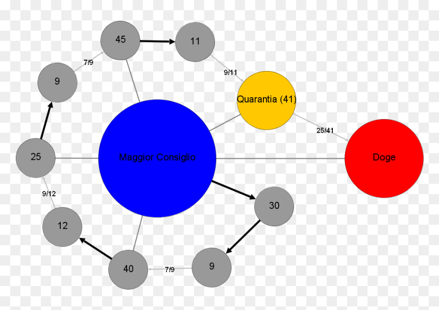
Now, let us describe the protocol : In this protocol, general simulates the protocol for all the generals in the first group, and analogously for the general and (see the video below). So, the three generals are simulating a protocol that was supposed to be run on generals. After the simulation of this protocol finishes, each of the three generals outputs the output of any of his simulated generals. This finishes the description of the protocol .

Why does solve the Byzantine generals problem in the case of one traitor? Well, it follows from the correctness of . I will leave the details to you, but importantly, if one of the three generals is a traitor, he can corrupt up to generals in the simulation of . But our assumption on that protocol implies that even that is not enough to break it, so the simulation of solves the consensus problem for the simulated generals which in turn implies the correctness of .

We conclude that if our theorem is true for , it is true for all .

Solving the case n=3

Ok, here comes the really fun part — how do we prove that the Byzantine generals problem is impossible for generals, one of them being a traitor? We will assume that a protocol solving the problem exists and derive a contradiction from this assumption.

The way we will do it is IMHO absolutely beautiful and I summed it up in the following animation.

Look, it is really important here to understand what a protocol is. Very formally speaking, our supposed protocol is a function that gets the following inputs.

1. How many generals are there? In this case,
2. Which general is this?
3. What step is this?
4. What messages arrived in steps ?

Given these inputs, the protocol outputs two messages that the general sends to its two neighbors with labels from in step . The insane idea of the proof is that we will take the protocol and run it in a way in which it is not supposed to be run at all.

Consider the following experiment. Instead of connecting the three generals to both its neighbors and running three copies of the protocol simultaneously, we will create a six-cycle. It will contain generals named with inputs . We will then run six copies of the same protocol on this six-cycle. Notice that there is no adversary in this experiment, all generals are following .

Although this can be done, it is not clear at all that the output of in this experiment has any meaning. In fact, as far as we know, the simulations of may crash, not terminate, or return some crap when we run them this way.

Next, focus on any two consecutive generals on the cycle — in the video, these are the two generals named at the top. Here is a cool observation: We can think of the remaining four generals as a single adversary! That is, we can think of the experiment as consisting of three parties connected with each other: the first two parties are the two top honest generals that follow the protocol and the third party is the remaining generals.

We can think of this third party as a traitor. But look, is supposed to work in the presence of a traitor! So we can conclude that the copies of the protocol run by the two top generals have to terminate. Moreover, since the two generals started with the same inputs , their outputs also have to be (see the next video). This is because of the requirement on correct protocols that if all honest generals started in a consensus, they cannot change their minds and have to output the same as the output.

But we can apply this thought experiment to any two consecutive generals. Namely, the generals at the bottom left (in the next video) have to output by the same reasoning. But what about the two top-left generals 1 and 3? As the protocol is correct, the two generals have to achieve consensus, i.e., they have to output the same number in our simulation. But we have just proven that one of the generals outputs , while the other one outputs , a contradiction!

Links

Distributed Computing Pearls by Gadi Taubenfeld — amazing book full of riddles from the area of distributed computing, including Two generals and Byzantine generals problem.

Distributed Computing by Nancy Lynch — a classic book on distributed computing.

1. It should be said that Latex is “just” a set of macros on top of Tex created by Donald Knuth. ︎
2. In the first snippet from Lamport, he calls it the “Chinese generals problem”. ︎
3. In the video, we also mentioned that blockchain-based protocols can solve the problem if less than n/2 generals are traitors. What’s going on? If the protocol is based on public cryptography, there is a hidden assumption in it – the public key of each general is common knowledge. But in the Byzantine generals problem as we defined it, this starting common knowledge is not allowed. Can we then start our public-key-based protocol by each general publishing his public key so that everybody agrees that they have the same copy of it? Well, if we could do that, then the general could instead publish his input and we would get a solution to the original Byzantine generals problem we are trying to solve. In other words, setting up public-key based protocols is at least as hard as the problem we are ultimately trying to solve. ︎

In the book Surely, You Are Joking, Mr. Feynman, Richard Feynman tells a story of how he provoked math students at Princeton by asking them to explain what problems they were working on. He would then tell them pretty much instantly what the answer to their problem is1. The catch is: just the answer, no proof. The whole point he was making was how mathematicians spend too much time formalizing proofs even though our intuition is already telling us what the answer should be.

But how does one develop such intuition? I want to tell you about one pretty general heuristical trick that I often find helpful. If I had to summarize the trick in a single sentence, I would probably say something like this:

If there is no reason for structure, assume there is none.

Instead of trying to define this more precisely, let me just list a bunch of applications of the trick, and let’s hope we get some intuition along the way. Except for the very end of the post, the applications are from number theory since those are simplest to explain.

Warning: We will use a lot of informal asymptotics. For example, I will say things like “There are roughly numbers of size roughly ”. By a number of size roughly , I mean that it is equal to up to some multiplicative constant. For example, numbers between and have size roughly , but is much larger than .

Fermat’s last theorem

Fermat’s last theorem says that for , we cannot find positive numbers such that ; I will call this equation Fermat’s equation from now on.

Let’s see why the theorem should be true. We will rely on the following intuition:

There is no reason why should be a -th power.

So we might conjecture that whenever it happens for some three positive numbers that , there is no deep reason for it, it’s just a coincidence, whatever that means.

Let’s now make this intuition quantitative. Start by splitting all triples into buckets so that the bucket gets all triples with . There is nothing deep to this bucketing, I am defining it because triples in the same bucket have roughly the same “probability” of satisfying Fermat’s equation. In the end, we are going to sum over all buckets, each time multiplying the size of the bucket by this “probability”, and this way we will get our estimate of how many solutions the equation has.

Let’s look at triples from some particular bucket . I will adopt the shorthand for brevity.

For any triple from bucket , the right-hand side of Fermat’s equation, , is roughly equal to because — to be more concrete, so but we don’t care about concrete constants.

Turning our attention to the left-hand side, notice that whenever or , the left-hand side is larger than the right-hand side, so the “probability” of such a triple satisfying the equation is zero.

What remains are triples where , i.e., both and are of size at most roughly . For those, the left-hand side of Fermat’s equation, , equals a number whose size is at most about . Here we finally come to the heuristic part of the argument. We will think of as a moving target: Instead of being a fixed number from the interval , we think of it as a random number sampled from the uniform distribution over . This heuristic is based on the intuition that the left-hand side of Fermat’s equation does not have anything to do with -th powers, so the only reason why we get a solution is a chance event.

We can now compute the probability of getting a solution to the equation to be about (this number is computed up to a constant, is regarded as a constant too). On the other hand, there are about relevant triples in the bucket . Thus, if we now count how many solutions we expect the -th bucket to contribute, we get that it is about .

To get the guess for the overall number of solutions, we need to sum up over all values of . So, our final guess is that, up to constant factors, the number of solutions is:

Let’s try to make sense out of this expression:

If or , then the expression goes to infinity as gets larger. So, our guess is that there are infinitely many solutions. You can check that this is correct and we are, in fact, even correctly guessing how quickly the number of solutions grows with the size of !2

For our sum converges pretty quickly to a constant. So we are expecting that if Fermat’s last theorem fails, it will be because there is some “sporadic” solution with pretty small a,b,c and k. After checking a few small cases, we would then conjecture that there should be no solutions which again turns out to be correct!

For , our sum goes to infinity, albeit pretty slowly. We are expecting that for numbers of size at most , there will be about solutions. This is a wrong guess.3

And that’s it! After multiplying a bunch of numbers, we got a pretty good guess on how Fermat’s last theorem goes for which values of . The infinite sum may look a bit complicated, but getting to the expression is the important part, after that we just need to check whether it grows at least as fast as . We failed for the special case where it grows exactly that fast but otherwise, the argument was spot on.

The biggest problem with the heuristic is that there may in fact be some structure in the original problem that we did not take into account. For example, if we choose , we would predict that there are tons of solutions to Fermat’s equation. Yet, 1+1 is never equal to 1. Or what if we allow to be nonnegative instead of positive? For every , we then have a ton of solutions of the type , but our argument still predicts there are almost none for any . Another example of a structure in the original problem is that whenever we find with , we get in fact an infinite family of solutions for any integer : our argument “does not know” about this fact.

This kind of heuristics unfortunately does not really help us with the actual proof of the theorem. But I think it is still pretty helpful. Some time back, I talked with a friend about the following question: If you know that Fermat’s last theorem holds for all (this was known before Wiles’ proof), how certain can you be that the theorem holds for all ? My friend’s position was that there are many more numbers between 100 and infinity than between 3 and 100. But I would say that the above argument suggests that we should still be quite sure that if Fermat’s last theorem fails, it will be much more probably because of k<100 than k>100. Thus, proving it for all k<100 should meaningfully update us on the theorem being true.

Try the heuristic yourself! Think about each problem before you click on the link.

1. Euler’s conjecture: Are there 5 integers such that ?
2. Catalan’s conjecture: Are there 4 integers such that ? If so, are there infinitely many of them?
3. Dirichlet’s approximation theorem: For which numbers do we expect the following to hold: For any irrational number , we can find infinitely many pairs of integers such that . [Hint: 4]
4. Square-sum problem: I give you a number . Is it possible to reorder the sequence so that any two consecutive numbers sum up to a square? [Hint: 5]
5. Collatz conjecture.

Magic squares of squares

A 3×3 magic square is a square with nine natural numbers such that all rows, all columns, and both diagonals sum up to the same number. Moreover, all 9 numbers should be different.

Do we expect there to be such a thing? We already know how to approach this problem! Let’s say that we look at the squares for which the sum of rows/columns is roughly $N$. Each entry of such a square is a number between and . So there are about such squares and we just need to estimate the probability that one particular square satisfies all constraints.

First, the nine numbers need to be pairwise different, but the probability of two random numbers of size ish being the same is only about , so the probability of this event is negligible. The serious constraints are those that say that rows, columns, and diagonals sum up to the same number.

With the notation from the picture, we can write down the constraints as:

There is some number such that:

1. 
2. 
3. 
4. 
5. 
6. 
7. 
8. 

So this is 8 constraints and each one of them has a probability about of being satisfied because is of size roughly . But saying that the probability of all constraints being satisfied is is not the way to go for two reasons.

First, even if there were just one constraint , the probability of it being satisfied would be 1, not 1/N. That’s because we are saying “There exists an ” which gives us a degree of freedom. We can solve this problem by instead defining . Then we can drop the first equation from the list and replace by on the right hand sides of the remaining equations.

The second problem is that our assumption that each equation is satisfied independently of the others is pretty wrong here. Look at the list above. The first three equations are saying that all numbers in the square sum to . The fourth and fifth equations are saying that the first two columns of the square sum up to . But these two facts imply that the third column sums up to . This means that we can kick out the equation from our list, it is implied by the equations above it.

Combining both observations, we simplify the list of constraints to:

1. 
2. 
3. 
4. 
5. 
6. 

At this point it finally (hopefully) makes sense to heuristically assume that there is no other dependence between these equations, so let’s just assume they are independent and let’s make the calculation of how many solutions we expect for numbers between and . We get . So we estimate that there are plenty of magic squares and we even estimate that their number grows as a cube power of the size of the numbers inside the square. This turns out to be the right estimate! 6

Let’s go on with something more interesting — what if we want each number inside the square to be a second power, i.e., a square? Our calculations are easy to adapt! We again estimate number of squares with numbers that are where something is a number between 1 and . There are again around of such squares, even after throwing away squares where the same number appears multiple times. On the other hand, we have the six constraints above that need to be satisfied. But now each one of them is satisfied only with probability about because the numbers in the square have size around . So we get that the number of such squares is about .

Remember, we just calculated the number of solutions for a particular scale, in the end we need to sum up over all the scales. We already did it with Fermat’s last theorem with using the bucketing approach. The upshot was that is the right threshold for whether we are expecting the solutions to exist or not. that we now computed is well below it, so we are expecting no such squares to exist (after we check that there is no such square for or so by brute force).

Ok, so let’s again see how good our method is by looking at what is known:

• There is no known 3×3 square of squares. It is known that if there is one, the numbers in it have to be absolutely gianormous. So it looks pretty good for our method here.
• What if we allow the magic square to have a wrong sum in one of the diagonals? We are predicting that there should be infinitely many of them, because , so their number should grow, albeit very slowly like . An example of such a square is the Parker square. However, this square does not use nine distinct numbers. I am not sure if there are known squares without this problem and how far people searched for the solutions. So it’s a bit unclear how to judge our prediction here.
• The method predicts that if you allow two numbers in the magic square to not be squares, then there should be infinitely many such squares since . As far as I understand, there is just one known example of such a square (up to symmetries), while we predict that their number should grow (very slowly) like . Again, it’s unclear what this means for our prediction.
• We predict that there should be examples of 4×4 squares of squares, because . There are a few known families of such squares, so this looks good.

Primes

A typical application of this method is to deal with primes. One of the most important number theoretical result is the so-called prime number theorem that says that there are about primes7 between 1 and . If we throw in the heuristical assumption that primes behave “kind of randomly”, we arrive at the heuristic that

A number is prime with probability about .

Here is a typical application: twin prime conjecture claims that there are infinitely many pairs where both and are primes. This makes sense — for each we can estimate that is prime with probability and is prime with probability . Our heuristic suggests that these two events are independent, so we can estimate that the probability of being twin primes is about . Hence, the number of twin primes should not only be infinite, but it should grow like , which seems to be spot on!

Try it yourself! Try to guess if the following statements are true.

1. Goldbach conjecture: Can every even number except of 2 be written as the sum of two primes?
2. Green-Tao theorem: Are there infinitely many pairs (n,k) such that is a prime?
3. Truncatable prime: Do you think there is a number n such that n modulo is prime for any k between 1 and 1000?
4. In the analysis of Erathostenes’ sieve, we get that its time complexity is . How fast does this sum grow? [Hint: 8]
5. abc conjecture: see the blog post of Terence Tao.

This model of primes has a name – Cramér’s random model. The Riemann hypothesis is equivalent to the claim that the prime number theorem is never wrong by more than roughly . If the random model were true, then this would indeed be roughly how much we would expect the prime number theorem to ever gowrong. So you can view the Riemann hypothesis as a way of trying to formalize the consequences of the random model of primes being a good model.

Does this thing have a name?

While this type of reasoning is ubiquitous, I am not sure whether there is some standard name for this kind of heuristic. Tao calls it “standard probabilistic heuristic argument“. In statistical physics, this general idea is called the mean-field model. There is also a cool paper trying to lay grounds for formalizing what does it mean to use this kind of heuristics. The paper calls this type of heuristic presumption of independence, because we can view applications of this reasoning as assuming that certain random variables are independent although they are not.

Footnotes

1. At least so the story goes. Somehow, all of Feynman’s stories have the common feature of Feynman coming out of them as the hero. ︎
2. For $latex k=2$, this follows from Euclid’s formula for Pythagorean triples. ︎
3. Check out this post for more discussion on this failure. ︎
4. Let $latex \alpha \in [0,1]$. For any $latex q$, think of all the numbers $latex 0/q, 1/q, \dots, q/q$ and draw a small interval of length $latex 1/q^\alpha$ around each of them. What is the total length of these intervals? What is the “probability” that these intervals contain $latex \alpha$? ︎
5. If you create a random graph by including each edge with probability $latex 100\log(n)/n$, the graph contains a Hamiltonian cycle with very high probability. ︎
6. In this particular case, it would perhaps be simpler to just solve the equations. ︎
7. In fact, I should write $latex n/\ln(n)$ to be more precise but we will not really need to care about constants here. ︎
8. First, use that $latex n$-th prime has size roughly $latex n \log(n)$ to write this as $latex 1/(2 \log 2) + 1/(3 \log 3) + \dots + 1/(n \log n)$. Remember how you can sum up the sum $latex 1/2 + 1/3 + \dots + 1/n$ by splitting it to intervals of length 1, 2, 4, … and use the trick also here. ︎

We made a new video with the Polylog team! As usual, there is quite a lot of stuff happening behind the scenes that did not fit in the final video. I decided to put that stuff in a separate blog post to satisfy both interested viewers and myself. If you did not watch the video, you should do that first!

If you make it to the end of the post, you will be rewarded with a description of the system for electing the doge which I find quite stunning.

Examples

Before diving in, let’s look at a few of the creatures we are talking about. In the video, we touched upon three voting systems: plurality voting (also known as first past the post or one-round election), the two-round system, and approval voting. Here are some additional voting systems you might be familiar with:

• Alternative vote/instant runoff/ranked choice voting — a generalization of the two-round system; instead of 2 rounds, you run (#candidates-1) rounds. In each round, you let every voter vote for their favorite and the candidate with the least votes drops from the race, you do this until only the winner remains. For practical reasons, voters vote only once and tell you their full preference ordering, then you simulate this process internally. Together with approval voting one of the most popular voting systems among voting theorists.
• Borda count — every voter orders the candidates. If you put a candidate to i-th place, then that candidate gets (n-i) votes from you. Sum up the votes for each candidate and order them by how many votes they got.
• Range voting — generalization of approval voting where you give any number between 0 and M of votes to each candidate, for some M. Sorting YouTube videos by how many likes they got, is an example of this system because giving -1, 0, or 1 vote is equivalent to giving 0, 1, or 2 votes.
• Range voting with average — The example above is a bit weird, maybe some video has 1000 views and 1000 likes and we put it below a video with 2000 views and 1001 likes although the viewers of the first one clearly enjoyed it more. Another option we have is to sort the videos by the ratio of #likes/#views. This corresponds to how we rank movies in top movie lists by their average rating. This makes sense if there are a lot of candidates to choose from, but it’s not that good for political elections — if the only person that cares enough about Joe Loser to even rate him is Joe himself, funny stuff can happen (similarly, top movie lists typically include only films with at least x reviews for some x).
• STAR voting — As in range voting, you are giving 0 to 5 stars to each candidate. The two candidates A, B with the most stars go into the final round where your vote goes to A if you gave her more stars than B, and vice versa. This system is not very well-known but for me, this is an example of a voting system where I find it extremely hard to come up with a plausible story of how we get strategic voting in real-world situations. Basically, the biggest problem with approval/range voting systems is that you can have two very strong candidates A, B and you like both of them but you like A a bit more than B. Then you have an incentive to give B zero votes so as to increase A’s probability of winning. But in STAR voting, you simply give 5 stars to A and 4 to B.
• Condorcet methods — In the video, we discussed how Condorcet cycles are the reason why all voting methods sometimes have undesirable properties. But maybe Condorcet cycles are quite rare in actual elections. Condorcet methods are trying to leverage that: they are supposed to work well in the absence of Condorcet cycles. In particular, whenever there is a candidate who beats everybody in a head-to-head election, this candidate should be elected as the winner by any voting system from this family. Many Condorcet methods are considered to be among the best voting systems we have – one of my favorites is Schulze method.

Our video also discussed a definition of a voting system that covers plurality and the two-round system but not approval voting (I will mention the more general definition later). Which of the above voting systems are captured by that definition? [Answer: 1 ]

Arrow’s theorem

If you believe that voting is important, I think you’ll also appreciate the significance of Arrow’s and the Gibbard-Satterthwaite theorem. Whenever you try to design a new voting system, compare existing ones, or think of what properties voting systems can have, these theorems are the place where you start.

I am not completely satisfied with how these theorems are usually introduced and discussed and this was the main motivation behind the video.

Let me share the standard introduction to Arrow’s theorem and then offer a bit different perspective that, in my opinion, provides better clarity. We will discuss the Gibbard-Satterthwaite theorem later.

Wikipedia has a nice article about Arrow’s theorem, I will now follow it. We will use the same definition of a voting system as in our video – the system gets candidate rankings from all voters as the input and sorts all candidates for the output.

There are a bunch of conditions that we want our voting system to have:

1. Non-dictatorship — the dictatorship system is the system that always outputs the preference of a single voter. We don’t want our system to be this system.
2. Pareto-efficiency — if every voter prefers A to B, so should the final order.
3. Independence of irrelevant alternatives (IIA) — as explained in the video, if I only tell you how each voter ranks A versus B, you should have enough information to conclude the relative order of A and B in the final outcome.

Now Arrow’s theorem says the following:

Arrow’s Theorem: For any number of voters and any number m>=3 candidates, the following is true. No voting system can satisfy all three conditions above.

Even better, for any two conditions there is a simple example of a voting system that satisfies both of them but not the third one. Let’s see those examples.

1. Drop Non-dictatorship: then you allow the dictatorship voting system that satisfies both 2 and 3.
2. Drop Pareto-efficiency: then you can have a system that is itself the dictator, i.e., for any input it returns always the same order of candidates; this system satisfies both 1 and 3.
3. Drop IIA: Pretty much every normal voting system (plurality, two-round, Borda count, …) satisfies 1 and 2, after you specify how to do symmetry breaking in case of a tie.

However, consider this: By disregarding conditions 1 and 2, we inadvertently permit systems that, from a practical standpoint, are highly flawed; they go completely against the spirit of the problem we are trying to understand here — the aggregation of opinions of many different actors.

Pretty much every voting system that deserves to be called a voting system satisfies 1 and 2, but not 3. So the way I think about Arrow’s theorem is: No reasonable voting system satisfies IIA, under a very mild definition of the word “reasonable”.

This perspective isn’t particularly controversial (cf. the Wiki page I linked). Still, our video tried to go further and explain Arrow and Gibbard-Satterthwaite without even mentioning the full statement of these theorems (in the case of Arrow this means the conditions 1 and 2 above). Why can this be helpful?

When discussing Arrow’s theorem with a bunch of friends, I felt they usually remembered that Arrow’s theorem says that no voting system can satisfy several conditions at once but who knows what they are. Sometimes I even heard “The only reasonable voting system is the dictatorship” which I think is a very unproductive take. I am pretty sure that even those who know the statement of Arrow’s theorem could not put together the proof of it – look at Wikipedia which explains two classical proofs of the theorem. Both of them are quite subtle and it is not easy to extract the main idea that you can remember.

What I would like my friends to remember about the theorem is: It says that no (reasonable) voting system can satisfy the independence of irrelevant alternatives. Also, the ultimate reason for that is Condorcet cycles. In fact, the existence of such cycles implies a weaker version of the theorem.

In fact, our video didn’t delve into the proof for the simplified version of Arrow’s theorem based on our definition of “reasonable.” Let me outline that for you. It’s basically the first half of the proof of Gibbard-Satterthwaite from the video – look at a Condorcet cycle and the voters that are unhappy about the result to find the contradiction.

Proof sketch of Arrow’s theorem with this definition: Assume that there are just three candidates, if there are even more of them, the proof stays the same. For any number of voters, there exists a Condorcet cycle with that many voters such that there are three groups of voters whose preferences are ABC (=prefer A over B over C), BCA, and CAB. Consider any reasonable voting system.

We can assume without loss of generality that A is the winner elected by the voting system in our Condorcet cycle; this is because the properties of Condorcet cycle are symmetric with respect to A, B, and C. Consider the voter group BCA and change their ballots to CBA. Our definition of “reasonable” and the property of the Condorcet cycle that each of the three groups has less than half of the voters together imply that C should be the winner in this new scenario. So A and C swap their relative order when we go from the original Condorcet cycle to the new scenario.

But this is forbidden by IIA which says that since B is an irrelevant alternative for A and C, voters changing their opinion of B should not lead to a swap in their relative order.

For me, this proof is pretty intuitive, so I think that if somebody wants to learn a bit about voting theory, it makes more sense to first see this proof and understand how it works, and only then see the general definition of Arrow’s theorem and the general proof of it.

Gibbard-Satterthwaite theorem

Our video was primarily about the Gibbard-Satterthwaite theorem, not Arrow. Let me first state the standard version of that theorem here:

Gibbard-Satterthwaite theorem: For any number of voters and any number number of candidates, consider any voting system such that at least three different outcomes are possible (= there are at least 3 different scenarios for which the system outputs different winners). Also, assume that that the voting system is not a dictatorship. Then this system sometimes incentivizes strategic voting.

You should parse the theorem as saying that any reasonable voting system sometimes incentivizes strategic voting, where the system is reasonable if at least 3 candidates can win (for example, if your voting system elects a candidate A in the case they are the first option of every voter, then your voting system has this property) and it is not a dictatorship of one voter.

For simplicity, the definition of a voting system we use for Gibbard-Satterthwaite is that we only want to elect the winner and not sort all candidates as in Arrow’s theorem. This doesn’t really matter — if your system can only elect the winner, you can always use it to find the winner, then use it one more time on the remaining candidates to find the second candidate, and so on until you get all candidates ordered. On the other hand, if you can sort candidates, as a special case you can elect the winner. So there is a natural way of switch between these two setups. 2

The discussion that we just had about Arrow’s theorem and how it’s more understandable if you first see a simpler version of it applies also to Gibbard-Satterthwaite. In fact, the usual formal proof of it utilizes Arrow’s theorem. This means that it takes quite a long time to prove it from scratch and that’s probably the reason why it’s surprisingly hard to find an explanation of Gibbard-Satterthwaite on the Internet. The full, formal proof simply does not fit in a short blog post/YouTube video.

This may be also the reason why Arrow’s theorem is much more famous than Gibbard-Satterthwaite. I am not very happy with this. Arrow’s theorem is incredibly important from the historical perspective — when Arrow proved it in the fifties, he basically kickstarted the field of voting systems theory — but I would say that the biggest reason why we should care about the IIA condition is that when it fails, it leads to strategic voting. Also, Arrow’s theorem works only for the definition of the voting system we used in our video, which does not cover the voting systems you are coming across most often (I am thinking of range voting systems, e.g., rating films, restaurants, and all kinds of other stuff). On the other hand, Gibbard-Satterthewaite covers all voting systems.

This place is probably as good as any other to explain the general definition of a voting system for which Gibbard-Satterthwaite still applies. In the general definition, every voter simply has some actions that they can do. For example, in approval voting with candidates, everybody has possible actions — you can give a vote to any subset of candidates. The voting system is simply a function that takes these actions as the input and it outputs the winner.

A voter v has the incentive to vote strategically means the following: If you fix the actions of all other voters than v one way, v wants to take some action  to make the system elect the best candidate according to v’s preference. On the other hand, if you fix the actions of all other voters a different way, v wants to take a different action .

Example: A bunch of people need to decide which film to go to, with three options A,B,C. You like A>B>C and are last to vote. If A and B are tied in the first place, you will vote for A. If B and C are tied in the first place, you will vote for B. This is strategic voting as defined above, i.e., your vote depends on the context of other votes.

Nonexample: In informal discussions, strategic voting is used a bit more broadly. For example, in our video, we gave an example where you give dislike to a video even though you kind of like it because you really want some other video to win. This is technically speaking not strategic voting according to our definition, at least if you do this same action in every possible context of other people’ ballots.

Going back to Gibbard-Satterthwaite theorem — it was proven in the early 70’s, independently by Satterthwaite who proved it for the weaker definition of a voting system used in the video, and Gibbard who proved it for the general definition of a voting system. This is why the general version of the theorem is known only as Gibbard’s theorem.

I want to stress how powerful Gibbard’s theorem is. It really works pretty much always and its conclusion is pretty strong.

A reasonable definition of “reasonable”?

When making the video, we had to think hard about the following problem.

What is the best definition of a “reasonable” voting system?

The question is of course not very well-defined, but we are looking for something like this:

1. The definition is intuitive.
2. It is satisfied by real voting systems people use.
3. It should make sense both for Arrow’s and the Gibbard-Satterthwaite theorem.
4. It should make their proofs simple.

There were two main candidates for the definition of “reasonable” that we considered, and I find neither of them completely satisfactory. Here they are.

1) “If a majority of voters votes for A, then A should be the winner”. This is the definition we in the end used in the video. It leads to simple proofs of both theorems, as you saw.

The main problem with this definition is that according to it, one of the voting systems we have seen so far is not reasonable (which one? Answer: 3). We hoped this shouldn’t be a dealbreaker for our video, but in general, I find this quite unsatisfactory.

2) “The system does not prefer any voter to another one. Also, it doesn’t prefer any candidate to another one. “ By this definition, I mean the following:

1. If the ballots that are the input to the system are arbitrarily permuted, the answer of the voting system should not change.
2. If you swap A and B on every ballot, then A and B should be swapped in the final order.

This is extremely elegant: All voting systems that we mentioned are designed to satisfy this property. But then again, there are systems that don’t. For example, the Council of the European Union uses the so-called double majority: you need at least 15 of 27 countries + at least 65% of EU population for your proposal to go through. The second condition fails our “reasonability” criteria since each country has a different weight.

But the biggest problem for us was this: No voting system can satisfy this definition! Ties are the problem. Basically, if you have just two voters, one prefers A to B and the other B to A, there is no way to elect the winner and keep this definition of “reasonability” satisfied. If you say that clearly nobody should be elected here and our definition of a voting system should include the possibility of ties, then you are completely right. But then all definitions become very clumsy. Also, what about the preschool teacher voting system that always outputs “everybody is the winner”? We need to add at least one more condition to our definition of “reasonable” to forbid this system.

As the other Václav from our Polylog team put it, our video already has “a lot of surface and not so much volume”, meaning a lot of definitions and not so much proof action going on.

So in the end we went for the first option, but I am not completely happy with it. If you can think of other interesting options to choose from, let me know in the comments! As far as I know, this is an interesting open exposition problem. 4

Takeaway

Our video was supposed to be accessible to as many people as possible, but there were also several more advanced and often neglected ideas that we tried to gesture at:

• If you ever voted strategically, it is not your fault — you are behaving rationally. But you can view it as a fault of the voting system.
• Arrow’s and the Gibbard-Satterthwaite theorems should be looked at as saying that “reasonable” systems fail to have some nice properties.
• The proofs of the theorems are not so complicated to understand if you don’t shoot for the most general definition of “reasonable”.
• Arrow’s theorem actually does not apply to many important voting systems.
• The Gibbard-Satterthwaite theorem is perhaps more interesting and fundamental than Arrow’s.
• Both theorems are worst-case in nature. They are good to know but this is just the beginning of a more complicated discussion of which voting systems fail how often and in which way.

If we managed to convey at least some of those points without confusing you, then we were successful.

The last point is especially important — although Arrow and Gibbard-Satterthwaite are very qualitative theorems (they apply to every voting system in the same way), the reality is more quantitative (some voting systems are better than others). Unfortunately, capturing that is pretty complicated.

Ultimately, what we care about is not strategic voting per se, it is something like: “If we use this voting system, on average, how happy are voters going to be with the result?” For example, the dictatorship voting system is bad because in many situations, most voters would be much happier if a different candidate was elected.

The important observation is that this fuzzy objective correlates with strategic voting — to give an example, plurality voting is a bad voting system because it leads to the so-called spoiler effect where a popular candidate A might not win only because voters “split” their votes between A and a similar candidate A’. But you can view this problem as a problem of strategic voting — voters are forced by the system to vote for A even if they like A’ a bit more. So strategic voting is a helpful way to understand problems with voting systems, but the objective we actually care about is something fuzzier, harder to describe, and to agree on. See this for more discussion.

As I said in the beginning, Arrow and Gibbard-Satterthwaite are the place where we start a discussion about voting systems. But it is just the start.

Bonus: Electing a doge

By a doge, I of course mean the leader of Venice.

Here is how the election process went.

“Whenever the time came to elect a new doge of Venice, an official went to pray in St. Mark’s Basilica, grabbed the first boy he could find in the piazza, and took him back to the ducal palace. The boy’s job was to draw lots to choose an electoral college from the members of Venice’s grand families, which was the first step in a performance that has been called tortuous, ridiculous, and profound. Here is how it went, more or less unchanged, for five hundred years, from 1268 until the end of the Venetian Republic.

Thirty electors were chosen by lot, and then a second lottery reduced them to nine, who nominated forty candidates in all, each of whom had to be approved by at least seven electors in order to pass to the next stage. The forty were pruned by lot to twelve, who nominated a total of twenty-five, who needed at least nine nominations each. The twenty-five were culled to nine, who picked an electoral college of forty-five, each with at least seven nominations. The forty-five became eleven, who chose a final college of forty-one. Each member proposed one candidate, all of whom were discussed and, if necessary, examined in person, whereupon each elector cast a vote for every candidate of whom he approved. The candidate with the most approvals was the winner, provided he had been endorsed by at least twenty-five of the forty-one.”

— Anthony Gottlieb, “Win or Lose,” The New Yorker.

And a diagram for those of you who don’t find the process crystal clear:

I think that this is actually a pretty good voting system. On the other hand, you can probably drop half of the intermediate steps and it will still work essentially the same.

Links

I am pretty sure there are some nice explanations of Arrow and Gibbard-Satterthwaite out there — if you know some, or if you know some nice sources related to voting theory, post them in the comments! Here are some links you might like.

https://olsak.blog.idnes.cz/blog.aspx?c=642275 — The video is inspired by Mirek’s story.

There is a very nice YouTube video with some examples of strategic voting in real-world systems.

Wulf Gaertner: A primer in social choice theory

Nisan, Roughgarden, Tardos, Vazirani: Algorithmic Game Theory

1. The first two systems and the last one. ︎
2. If you are into fancy comparisons: This is pretty much the same argument as why the axiom of choice is equivalent to the well-ordering principle. ︎
3. Borda count. ︎
4.  The term is taken from here. ︎