Gábor Melis' Blog

Version 0.5 of DRef, the definition reifier, is now available. It has moved to its own repository, completing its separation from PAX, where it was originally developed.

This was a long time coming. Twelve years ago today, PAX was born. From the start, PAX used the concept of locatives to refer to definitions without first-class objects. For example, to generate documentation for the *MY-VAR* variable, one could use the VARIABLE locative as in (*MY-VAR* VARIABLE). PAX needed to be able to tell whether such a definition exists, as well as access its docstring and source location.

Over time, this mechanism evolved into a portable, extensible introspection library independent of PAX. I began separating the two projects two years ago and named the new library, though they continued to share a repository. I have now removed the remaining dependencies so that DRef can live on its own.

Classical literate programming

A literate program intersperses narrative and code chunks. From this, source code to be fed to the compiler is generated by a process called tangling, and documentation by weaving. The specifics of tangling vary, but by allowing complete reordering and textual combination of chunks, it lets the human narrative drive the exposition at the cost of introducing an additional step into the write-compile-run cycle.

The general idea

It is easy to mistake this classical implementation of literate programming for the more general idea that we want to

1. present code to human readers in pedagogical order with narrative added, and

2. make changing code and its documentation together easy.

The advantages of literate programming follow from these desiderata.

Untangled LP

In many languages today, code order is far more flexible than in the era of early literate programming, so the narrative order can be approximated to some degree using docstrings and comments. Code and its documentation are side by side, so changing them together should also be easy. Since the normal source code now acts as the LP source, there is no more tangling in the programming loop. This is explored in more detail here.

Pros and cons

Having no tangling is a great benefit, as we get to keep our usual programming environment and tooling. On the other hand, bare-bones untangled LP faces the following potential problems.

1. Order mismatch: Things like inline functions and global variables may need to be defined before use. So, code order tends to deviate from narrative order to some degree.

2. Reduced locality: Our main tool to sync code and narrative is factoring out small, meaningful functions, which is just good programming style anyway. However, this may be undesirable for reasons of performance or readability. In such a case, we might end up with a larger function. Now, if we have only a single docstring for it, then it can be non-obvious which part of the code a sentence in the docstring refers to because of their distance and the presence of other parts.

3. No source code only view: Sometimes we want to see only the code. In classical LP, we can look at the tangled file. In untangled LP, editor support for hiding the narrative is the obvious solution.

4. No generated documentation: There is no more tangling nor weaving, but we still need another tool to generate documentation. Crucially, generating documentation is not in the main programming loop.

In general, whether classical or untangled LP is better depends on the severity of the above issues in the particular programming environment.

The Lisp and PAX view

MGL-PAX, a Common Lisp untangled LP solution, aims to minimize the above problems and fill in the gaps left by dropping tangling.

1. Order

   • Common Lisp is quite relaxed about the order of function definitions, but not so much about DEFMACRO, DEFVAR, DEFPARAMETER, DEFCONSTANT, DEFTYPE , DEFCLASS, DEFSTRUCT, DEFINE-COMPILER-MACRO, SET-MACRO-CHARACTER, SET-DISPATCH-MACRO-CHARACTER, DEFPACKAGE. However, code order can for the most part follow narrative order. In practice, we end up with some DEFVARs far from their parent DEFSECTIONs (but DECLAIM SPECIAL helps).

   • DEFSECTION controls documentation order. The references to Lisp definitions in DEFSECTION determine narrative order independently from the code order. This allows the few ordering problems to be patched over in the generated documentation.

   • Furthermore, because DEFSECTION can handle the exporting of symbols, we can declare the public interface piecemeal, right next to the relevant definitions, rather than in a monolithic DEFPACKAGE

2. Locality

   • Lisp macros replace chunks in the rare, complex cases where a chunk is not a straightforward text substitution but takes parameters. Unlike text-based LP chunks, macros must operate on valid syntax trees (S-expressions), so they cannot be used to inject arbitrary text fragments (e.g. an unclosed parenthesis).

     This constraint forces us to organize code into meaningful, syntactic units rather than arbitrary textual fragments, which results in more robust code. Within these units, macros allow us to reshape the syntax tree directly, handling scoping properly where text interpolation would fail.

   • PAX's NOTE is an extractable, named comment. NOTE can interleave with code within e.g. functions to minimize the distance between the logic and its documentation.

   • Also, PAX hooks into the development to provide easy navigation in the documentation tree.

3. Source code only view: PAX supports hiding verbose documentation (sections, docstrings, comments) in the editor.

4. Generating documentation

   • PAX extracts docstrings, NOTEs and combines them with narrative glue in DEFSECTIONs.

   • Documentation can be generated as static HTML/PDF files for offline reading or browsed live (in an Emacs buffer or via an in-built web server) during development.

   • LaTeX math is supported in both PDF and HTML (via MathJax, whether live or offline).

In summary, PAX accepts a minimal deviation in code/narrative order but retains the original, interactive Lisp environment (e.g. SLIME/Sly), through which it offers optional convenience features like extended navigation, live browsing, and hiding documentation in code. In return, we give up easy fine-grained control over typesetting the documentation – a price well worth paying in Common Lisp.

Thanks to Paul A. Patience, PAX now has PDF support. See pax-manual-v0.4.1.pdf and dref-manual-v0.4.1.pdf. The PDF is very similar to the HTML, even down to the locative types (e.g [function]) being linked to the sources on GitHub, but cross-linking between PDFs doesn't work reliably on most viewers, so that's disabled. Also, for reading PDFs so heavy on internal linking to be enjoyable, one needs a viewer that supports going back within the PDF (not the case with Chrome at the moment). Here is a blurry screenshot to entice:

There is a bit of a Christmas tree effect due to syntax highlighting and the colouring of the links. Blue links are internal to the PDF, maroon links are external. I might want to change that to make it look more like the HTML, but I have not found a way in LaTeX to underline text without breaking automatic hyphenation.

At ELS 2024, I gave a talk on adaptive hashing, which focusses on making general purpose hash tables faster and more robust at the same time.

Theory vs Practice

Hash table theory most concerns itself with the asymptotic worst-case cost with a hash function chosen randomly from a family of hash functions. Although these results are very relevant in practice,

• those pesky constant factors, that the big-O cost ignores, do matter, and

• we don't pick hash functions randomly but fix the hash function for the lifetime of the hash table.

There are Perfect Hashing algorithms, that choose an optimal hash function for a given set of keys. The drawback is that they either require the set of keys to be fixed or they are too slow to be used as general purpose hash tables.

Still, the idea that we can do better by adapting the hash function to the actual keys is key. Can we do that online, that is, while the hash table is being used? Potential performance gains come from improving the constant factors mentioned above by

• having fewer collisions, and

  

• being more cache-friendly.

  

The first image above plots the regret (the expected number of comparisons of per lookup minus the minimum achievable) and the measured run-time of PUT operations vs the number of keys in the hash table with a particular key distribution. Green is Murmur (a robust hash function), Blue is SBCL's expedient EQ hash. The wiggling of the graphs is due to the resizing of the hash table as keys are added to it.

Note how SBCL's regret starts out much lower and becomes much higher than that of Murmur, but if anything, its advantage in run time (second image) grows.

Implementation

The general idea is sound, but turning it into real performance gains is hard due to the cost of choosing a hash function and switching to it. First, we have to make some assumption about the distribution of keys. In fact, default hash functions in language runtimes often make such assumptions to make the common cases faster, usually at the cost of weakened worst-case guarantees.

The rest of this post is about how SBCL's built-in hash tables, which had been reasonably fast, were modified. The core switching mechanism looks at

• the length of the collision chain on PUT operations,

• the collision count on rehash (when the hash table is grown), and

• the size of the hash table.

Adapting EQ hash tables

1. Init to to constant hash function. This a fancy way of saying that we do linear search in a vector internally. This is an EQ hash table, so key comparison is as single assembly instruction.

2. When the hash table is grown to more than 32 keys and it must be rehashed anyway, we switch to a hash function that does a single right shift with the number of bits to shift determined from the longest common run of low-bits in the keys.

3. If too many collisions, we switch to the previous default SBCL EQ-hash function that has been tuned for a long time.

4. If too many collisions, we switch to Murmur, a general purpose hash. We could also go all the way to cryptographic hashes.

In step 2, the hash function with the single shift fits the memory allocator's behaviour nicely: it is a perfect hash for keys forming arithmetic sequences, which is often approximately true for objects of the same type allocated in a loop.

In this figure, the red line is the adaptive hash.

Adapting EQUAL hash tables

For composite keys, running the hash function is the main cost. Adaptive hashing does the following.

• For string keys, hash only the first and last 2 characters.

• For list keys, only hash the first 4 elements.

• If too many collisions, double the limit.

So, SBCL hash tables have been adaptive for almost a year now, gaining some speed in common cases, and robustness in others.

The full paper is here.

Version 0.4 of PAX, the documentation system, and DRef, the definition reifier, was released. There were large refactorings, bug fixes, minor features, cosmetics, documentation and performance improvements too numerous to list.

Here is a summary of the new features and notable changes.

• DRef now supports DTYPEs, which allow filtering DEFINITIONS and DREF-APROPOS results according to the locative type hierarchy:

  (definitions 'print)
  ==> (#<DREF PRINT FUNCTION>
  -->  #<DREF PRINT (UNKNOWN (:DEFOPTIMIZER PRINT SB-C:DERIVE-TYPE))>
  -->  #<DREF PRINT (UNKNOWN
  -->                (DECLAIM PRINT
  -->                         SB-C:DEFKNOWN))>)

  (definitions 'print :dtype '(and t (not unknown)))
  ==> (#<DREF PRINT FUNCTION>)

  The AND T bit restricts the query to definitions in the running Lisp. The top of the DTYPE hierarchy is DREF:TOP, which includes external definitions such as the CLHS, that comes with PAX:

  (definitions 'print :dtype '(not unknown))
  ==> (#<DREF PRINT (CLHS FUNCTION)> #<DREF PRINT FUNCTION>)

  (dref-apropos "method" :package :dref :external-only t :dtype 'class)
  ==> (#<DREF METHOD CLASS> #<DREF METHOD-COMBINATION CLASS>)

  The locative type hierarchy can be queried programmatically, and this information is included in their documentation (see for example the GENERIC-FUNCTION locative type).

• The PAX Live Home Page better supports exploration without having to leave the browser. See the video.

  • It lists packages grouped by ASDF systems that define them (when this can be determined from the source locations).

  • It links to apropos pages for each locative type.

  • It has an input box for looking up documentation right from the browser (as if with mgl-pax-document from Emacs).

  • It has an input box for looking up apropos right from the browser (as if with mgl-pax-apropos from Emacs).

  • The web server can be started without Emacs.

• Completion of names and locatives in Emacs is much improved.

• New aliases were added to the CLHS pages documenting format directives (e.g. ~F), standard macro characters (#A) and loop keywords (sum, :sum, loop:sum), so that one can just C-. (mgl-pax-document) them. See the documentation of the CLHS locative.

• The DRef extension api has been cleaned up.

Over at argmin.net, Ben Recht is reflecting on Meehl's lectures on the metatheory of science, which is about how science progresses. The original lectures are fascinating but also long as well as long-winded, and I found Ben's blog series a much better read (especially since the originals are video recordings). Still, at the time of writing, with 13 blog posts covering less than half of the lectures (5/12), no self-respecting 21st century scientist can risk the time investment (equivalent to publishing 0.25 papers in machine learning) or – even worse – getting slowed down by methodological considerations.

So, here is my TLDR suitable for the short-haul commuter and the busy senior executive: it's all Bayes and incentives. There is no silver bullet method, and while we do questionable things for all the wrong reasons, time will clean up any mess that we make anyway.

Expanding that for slightly longer attention spans:

• Theories can be disproved but cannot be proved.

• We can only accumulate evidence that supports a theory.

• Evidence is subjective.

• All theories are wrong, but some are useful.

• The utility of a theory is its only grounding in reality.

At this point, the rest is somewhat predictable; my armchair is like any other. But if you can tolerate examples and spelling out implications, read on.

• We want to run convincing experiments, but what is convincing to someone depends on their beliefs about the possible hypotheses, results and what they know about our methodology (never fully specified) and us (e.g. motivations, beliefs, funding).

• We choose experiments to rule out large swaths of the hypothesis space weighted by our beliefs, which might bear little resemblance to others' beliefs.

• If the hypothesis space is large and we don't have very strong beliefs, it may be that we don't even think in terms of hypotheses. Instead, we may think in terms of probability of results (as if we marginalized out the hypotheses). "Hey, these results hold to 37 decimal places! What do you think the chances of that are if our model was wrong?"

• The entire process that produced a result is considered in belief updates. This includes the researcher, the machinery, the funding agency, the organization, etc.

• With so many factors, there is always room for different interpretations of results. Eventually, theories die when they are no longer useful (for any purpose).

• Classical formal logic has limited use in this setting. It seems to be all Bayes with a bit of decision/game theory thrown in.

• In these Bayesian belief updates, perceived incentives play a prominent role: many results are downweighted because we know the twisted academic and applied research incentive structure.

I believe improving the incentives is the most important contribution one can make in today's world. Now, go and read Ben's posts.

Catchy title, innit? I came up with it while trying to name the development style PAX enables. The original idea was something vaguely self-explanatory in a straight out of a marketing department kind of way, with tendrils right into your unconscious. Documentation-driven development sounded just the thing, but it's already taken. Luckily, I came to realize that neither documentation nor any other single thing should drive development. Less luckily for the philosophically disinclined, this epiphany unleashed my inner Richard P. Gabriel. I reckon if there is a point to what follows, it's abstract enough to make it hard to tell.

In programming, there is always a formalization step involved: we must go from idea to code. Very rarely, we have a formal definition of the problem, but apart from purely theoretical exercises, formalization always involves a jump of faith. It's like math word problems: the translation from natural to formal language is out of scope for formal methods.

We strive to shorten the jump by looking at the solution carefully from different angles (code, docs, specs), by poking at it and observing its behaviour (tests, logs, input-output, debugging). These facets (descriptive or behavioural) of the solution are redundant with the code and each other. This redundancy is our main tool to shorten the jump. Ultimately, some faith will still be required, but the hope is that if a thing looks good from several angles and behaves well, then it's likely to be a good solution. Programming is empirical.

Tests, on the abstract level, have the same primary job as any other facet: constrain the solution by introducing redundancy. If automatic, they have useful properties: 1. they are cheap to run; 2. inconsistencies between code and tests are found automatically; 3. they exert pressure to keep the code easily testable (when tracking test coverage); 4. sometimes it's easiest to start with writing the tests. On the other hand, tests incur a maintenance cost (often small compared to the gains).

Unlike tests, documentation is mostly in natural language. This has the following considerable disadvantages: documentation is expensive to write and to check (must be read and compared to the implementation, which involves humans for a short while longer), consequently, it easily diverges from the code. It seems like the wrong kind of redundancy. On the positive side, 1. it is valuable for users (e.g. user manual) and also for the programmer to understand the intention; 2. it encourages easily explainable designs; 3. sometimes it's easiest to start with writing the documentation.

Like tests or any other facet, documentation is not always needed, it can drive the development process, or it can lag. But it is a tremendously useful tool to encourage clean design and keep the code comprehensible.

Writing and maintaining good documentation is costly, but the cost can vary greatly. Knuth's Literate Programming took the very opinionated stance of treating documentation of internals as the primary product, which is a great fit for certain types of problems. PAX is much more mellow. It does not require a complete overhaul of the development process or tooling; giving up interactive development would be too high a price. PAX is chiefly about reducing the distance between code and its documentation, so that they can be changed together. By doing so, it reduces the maintenance cost, improves both the design and the documentation, while making the code more comprehensible.

In summary,

• Multiple, redundant facets are needed to have confidence in a solution.

• Maintaining them has a cost.

• This cost shapes the solution.

• There is no universally good set of facets.

• There need not be a primary facet to drive development.

• We mentally switch between facets frequently.

• Our tools should make working with multiple facets easier.

This is what PAX tries to do for documentation and code.
And that's the best 4KiB name I could come up with.

Try, my test anti-framework, has just got light Emacs integration.

Consider the following test:

(deftest test-foo ()
  (is (equal "xxx" 5))
  (is (equal 7 7))
  (with-failure-expected (t)
    (is (same-set-p '(1) '(2)))))

The test can be run from Lisp with (test-foo) (interactive debugging) or (try 'test-foo) (non-interactive), but now there is a third option: run it from Emacs and get a couple of conveniences in return. In particular, with M-x mgl-try then entering test-foo, a new buffer pops up with the test output, which is font-locked based on the type of the outcome. The buffer also has outline minor mode, which matches the hierarchical structure of the output.

The buffer's major mode is Lisp, so M-. and all the usual key bindings work. In additition, a couple of keys bound to navigation commands are available. See the documentation for the details. Note that Quicklisp has an older version of Try that does not have Emacs integration, so you'll need to use https://github.com/melisgl/try until the next Quicklisp release.

DEFSECTION needs to refer to definitions that do not create a first-class object (e.g. stuff like (*DOCUMENT-LINK-TO-HYPERSPEC* VARIABLE)), and since its original release in 2014, a substantial part of PAX dealt with locatives and references, which reify definitions. This release finally factors that code out into a library called DRef, allowing PAX to focus on documentation. Being very young, DRef lives under adult supervision, in a subdirectory of the PAX repository.

UPDATE – See DRef Leaves Home.

DREF> (definitions 'pax:document-object*)
(#<DREF DOCUMENT-OBJECT* GENERIC-FUNCTION>
 #<DREF DOCUMENT-OBJECT* (METHOD :BEFORE (OVERVIEW T))>
 #<DREF DOCUMENT-OBJECT* (METHOD :BEFORE (CATEGORY T))>
 #<DREF DOCUMENT-OBJECT* (METHOD (DYNAMIC-SECTION T))>
 #<DREF DOCUMENT-OBJECT* (METHOD (DREF-EXT:UNKNOWN-DREF T))>
 #<DREF DOCUMENT-OBJECT* (METHOD (MGL-PAX::CLHS-DREF T))>
 #<DREF DOCUMENT-OBJECT* (METHOD (MGL-PAX::INCLUDE-DREF T))>
 #<DREF DOCUMENT-OBJECT* (METHOD (MGL-PAX::GO-DREF T))>
 #<DREF DOCUMENT-OBJECT* (METHOD (GLOSSARY-TERM T))>
 #<DREF DOCUMENT-OBJECT* (METHOD (SECTION T))>
 #<DREF DOCUMENT-OBJECT* (METHOD (DREF-EXT:LOCATIVE-DREF T))>
 #<DREF DOCUMENT-OBJECT* (METHOD (DREF-EXT:PACKAGE-DREF T))>
 #<DREF DOCUMENT-OBJECT* (METHOD (DREF-EXT:ASDF-SYSTEM-DREF T))>
 #<DREF DOCUMENT-OBJECT* (METHOD (DREF-EXT:CONDITION-DREF T))>
 #<DREF DOCUMENT-OBJECT* (METHOD (DREF-EXT:CLASS-DREF T))>
 #<DREF DOCUMENT-OBJECT* (METHOD (DREF-EXT:STRUCTURE-DREF T))>
 #<DREF DOCUMENT-OBJECT* (METHOD (DREF-EXT:STRUCTURE-ACCESSOR-DREF T))>
 #<DREF DOCUMENT-OBJECT* (METHOD (DREF-EXT:WRITER-DREF T))>
 #<DREF DOCUMENT-OBJECT* (METHOD (DREF-EXT:READER-DREF T))>
 #<DREF DOCUMENT-OBJECT* (METHOD (DREF-EXT:ACCESSOR-DREF T))>
 #<DREF DOCUMENT-OBJECT* (METHOD (DREF-EXT:METHOD-DREF T))>
 #<DREF DOCUMENT-OBJECT* (METHOD (DREF-EXT:SETF-DREF T))>
 #<DREF DOCUMENT-OBJECT* (METHOD (DREF-EXT:VARIABLE-DREF T))>
 #<DREF DOCUMENT-OBJECT* (METHOD (DREF T))>
 #<DREF DOCUMENT-OBJECT* (METHOD (T T))>)

DREF> (dref 'pax:document-object* '(method (class-dref t)))
#<DREF DOCUMENT-OBJECT* (METHOD (CLASS-DREF T))>

DREF> (arglist *)
(DREF STREAM)
:ORDINARY

DREF> (docstring **)
"For definitions with a CLASS locative, the arglist printed is the
list of immediate superclasses with STANDARD-OBJECT, CONDITION and
non-exported symbols omitted."

DREF> (pax:document ***)
- [method] DOCUMENT-OBJECT* (DREF CLASS-DREF) STREAM

    For definitions with a CLASS locative, the arglist printed is the
    list of immediate superclasses with STANDARD-OBJECT, CONDITION and
    non-exported symbols omitted.

During the refactoring, the references API was cleaned up. How to write extensions has seen lots of changes (see Extending DRef and Extending PAX), but normal use is the same. DRef is similar to Shinmera's Definitions library but is more tailored to the needs of PAX.

Also in this release:

• Apropos got a detailed view feature, which includes the docstrings of all listed definitions not just the reference itself. This is very useful for getting an overview of a package.

  

• The detailed view often has to render docstrings which have not been written with PAX in mind and are not proper markdown. These docstrings are now sanitized aggressively in a unavoidably heuristic manner.

• There are now two supported CSS styles for HTML output: :DEFAULT with sans-serif and :CHARTER with Charter as the main font (which is bundled). The :CHARTER style is used in the linked PAX World documentation on this blog. See PAX:*BROWSE-HTML-STYLE* and PAX:UPDATE-ASDF-SYSTEM-HTML-DOCS.

• As usual, quite a few bug fixes and some optimizations also found their way into this release.

PAX got a live documentation browser to make documentation generation a more interactive experience. A great thing about Lisp development is changing a single function and quickly seeing how it behaves without the delay of a full recompile. Previously, editing a docstring required regenerating the full documentation to see how the changes turned out. The live documentation browser does away with this step, which tightens the edit/document loop.

PAX also got an apropos browser. It could always generate documentation for stuff not written with PAX in mind, so with the live browser already implemented, this was a just a small add-on.

The trouble with interactivity is, of course, that it's difficult to get the point across in text, so I made two short videos that demonstrate the basics.

• Live browsing with w3m

• Live browsing with other browsers

I put the sources of the Two-Tailed Averaging paper on github. Of course, the sources are also available on arxiv, but this may give better visibility to the LaTeX grid typesetting code in there. Also, note how much cleaner the paper looks with the XCharter font compared to Times New Roman. No wonder Matthew Butterick pushes Charter. By the way, see what he has to say about grids and baseline grids, in particular.

In short, comparing fonts at the same font size is almost never the right thing to do. Compare them at the same x-height or, better yet, at the same space usage.

In full, recently I wanted to choose a font that looks good on screen at various resolutions and also in print. This is fairly subjective, of course, so there is a lot of noise out there. Going by the LaTeX Font Catalogue, Google Fonts and similar font comparison sites turned out to be fairly misleading because they present fonts at the same font size (em in LaTeX and CSS). The problem is that 1em is the size of a bounding box for the largest character, which can be arbitrarily loose. The perceived size of typical English text is much more closely determined by the x-height (ex in LaTeX and CSS). 1ex is the height of the character x, which is pretty close to the height of other lowercase characters for most fonts.

So it makes a lot of sense to compare fonts at the same x-height, and this is what I first did for a number of LaTeX fonts: fonts-by-x-height.pdf. On the other hand, normalizing for x-height can make fonts with wider glyphs look much bigger in the eye of the beholder. Thus, the obvious alternative is to normalize the space usage. Unfortunately, there is no convenient statistic available for this, so we have to resort to estimating the area required to set a given piece of reference text with a given font. The advantage of this method is that it takes kerning into account, the disadvantage is that we must now choose the line height, which is quite an art in itself. Based on the assumption that the amount visual separation between lines is the main factor that determines the difficulty of scanning lines, here I decided to keep the ratio of line height and x-height constant. Of course, other factors such as cap height, ascenders, and descenders also matter in general, but for the fonts considered, they didn't vary strongly enough in addition to x-height to make them change the results: fonts-by-space.pdf. Have a look and decide for yourself which fonts look best. To me, the most legible fonts are:

• Libertinus and Stix2 in the Timeslike category,

• Cochineal (Amiri, Crimson Text) among the Garamondlike,

• XCharter among the (almost) Slab Serifs,

• Utopia among the Transitional Serifs.

My taste is apparently quite similar to Lino Ferreira's. EB Garamond is a personal favourite, but it is just a bit too quirky for body text. Those same quirks make it great at larger sizes though, and this blog uses it for headings in addition to XCharter for the body text.

The messy LaTeX sources of the above documents are available on github.

Comment on Twitter or Mastodon.

This is a complement to the Two-Tailed Averaging paper, approached from the direction of what I think is a fairly common technique: averaging checkpoints.

We want to speed up training and improve generalization. One way to do that is by averaging weights from optimization, and that's a big win (e.g. 1, 2, 3). For example, while training a language model for the down-stream task of summarization, we can save checkpoints periodically and average the model weights from the last 10 or so checkpoints to produce the final solution. This is pretty much what Stochastic Weight Averaging (SWA) does.

Problems with SWA

There is a number of problems with SWA:

• The averaging length (e.g. 10) must be chosen to maximize performance on summarization.

• A naive way to find the averaging length is to do a single training run and then search backwards extending the average one checkpoint at a time, which needs lots of storage and computation. Another option, doing multiple training runs each told to start averaging at a predefined point pays a steep price in computation for lower storage costs.

• To control the costs, we can lower checkpointing fequency, but does that make results worse? We can test it with multiple training runs and pay the cost there.

• Also, how do we know when to stop training? We ideally want to stop training the language model when summarization works best with the optimal averaging length at that point. That means the naive search has to be run periodically making it even more expensive.

In summary, working with SWA is tricky because:

• The averaging length is a hyperparameter that's costly to set (it is coupled with other hyperparameters especially with the length of training and the learning rate).

• Determining the averaging length after training is both costly (in storage and/or computation) and suboptimal (can miss early solutions).

These are the issues Two-Tailed Averaging tackles.

Two-Tailed Averaging

The algorithm needs storage for only two sets of weights (constant storage cost) and performance (e.g. of summarization) to be evaluated periodically. In return, it provides a weight average of approximately optimal length at all optimization steps. Now we can start training that language model, periodically evaluating how the averaged weights are doing at summarization. We can stop the training run any time if it's getting worse.

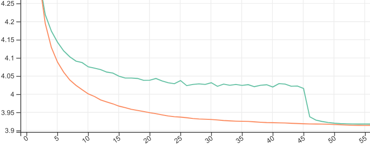
This is how Two-Tailed Averaged (orange) compares to SWA (green) tuned to start averaging at the point that's optimal for final validation loss:

The Algorithm

The core algorithm maintains two weight averages. Both averages are over the most recent weights weight produced by the optimizer, but they differ in length (i.e. how many weights they average). As the optimizer produces new sets of weights, they are added to both averages. We periodically evaluate the performance of our model with each average. If the short average (the one that currently has fewer weights averaged) does at least as well as the long average according to some arbitrary evaluation function, then we empty the long average, which will now be the short one.

# Initialize the short (s, sw) and long averages (l, lw). s and l are
# the number of weights averaged (the "averaging lengths"). sw and lw
# are the averaged weights.
s, sw, l, lw = 0, 0, 0, 0

# Update the averages with the latest weights from the optimizer.
def update_2ta(w):
  global s, sw, l, lw
  assert s <= l
  s, sw = s+1, (s*sw + w)/(s+1)
  l, lw = l+1, (l*lw + w)/(l+1)

# Evaluate the model with the short-, the long-, and the
# non-averaged weights. Based on the results, adapt the length of
# the averages. Return three values: the best evaluation results,
# the corresponding weights and averaging length.
def evaluate_2ta(w, evaluate):
  global s, sw, l, lw
  # Evaluate the non-averaged weights w, the short and the long average.
  f1, fs, fl = evaluate(w), evaluate(sw), evaluate(lw)
  is_first_eval = (s == l)
  # If the short average is better, then *switch*: empty the long
  # average, which is now the shorter one.
  if fs <= fl:
    s, l, lw, fl = 0, s, sw, fs
  if f1 <= fl:
    # The non-averaged weights performed better. This may happen in
    # the very early stages of training.
    if is_first_eval:
      # If there has never been a switch (s == l), then f1 is probably
      # still improving fast so reset both averages.
      s, l = 0, 0
    return f1, w, 1
  else:
    # Return the long average.
    return fl, lw, l

In addition to the core algorithm, the code above has some extra logic to deal with the non-averaged weights being better than the averaged ones.

Let's write a fake a training loop that optimizes \(f(x)=x^2\).

import random

def test_2ta_simple():
  def f(w):
    return w**2
  def df_dw(w):
    # Simulate stochasticity due to e.g. minibatching.
    return 2*w + random.uniform(-1.0, 1.0)
  lr = 0.5
  w = 3.14
  for i in range(1, 2001):
    w = w - lr*df_dw(w)
    update_2ta(w)
    if i % 100 == 0:
      f_2ta, w_2ta, l_2ta = evaluate_2ta(w, f)
      print(f'i={i:4d}: f(w_i)={f(w):7.3f},'
            f' f(w_2ta)={f_2ta:7.3f}, l={l_2ta:4d}')

We added some noise to the gradients in df_dw to make it more like training a neural net with SGD. Anyway, we take 2000 optimization steps, calling update_2ta on most but calling update_and_evaluate_2ta every 100 steps. Running test_2ta_simple, we get something like this:

i= 100: f(w_i)=0.108, f(w_2ta)=0.000, l= 100
i= 200: f(w_i)=0.011, f(w_2ta)=0.000, l= 200
i= 300: f(w_i)=0.098, f(w_2ta)=0.000, l= 200
i= 400: f(w_i)=0.085, f(w_2ta)=0.000, l= 300
i= 500: f(w_i)=0.221, f(w_2ta)=0.000, l= 200
i= 600: f(w_i)=0.185, f(w_2ta)=0.000, l= 300
i= 700: f(w_i)=0.019, f(w_2ta)=0.000, l= 400
i= 800: f(w_i)=0.180, f(w_2ta)=0.000, l= 500
i= 900: f(w_i)=0.161, f(w_2ta)=0.000, l= 600
i=1000: f(w_i)=0.183, f(w_2ta)=0.000, l= 700
i=1100: f(w_i)=0.057, f(w_2ta)=0.000, l= 800
i=1200: f(w_i)=0.045, f(w_2ta)=0.000, l= 900
i=1300: f(w_i)=0.051, f(w_2ta)=0.000, l=1000
i=1400: f(w_i)=0.010, f(w_2ta)=0.000, l= 900
i=1500: f(w_i)=0.012, f(w_2ta)=0.000, l=1000
i=1600: f(w_i)=0.168, f(w_2ta)=0.000, l=1100
i=1700: f(w_i)=0.001, f(w_2ta)=0.000, l=1200
i=1800: f(w_i)=0.020, f(w_2ta)=0.000, l=1300
i=1900: f(w_i)=0.090, f(w_2ta)=0.000, l=1400
i=2000: f(w_i)=0.115, f(w_2ta)=0.000, l=1500

In the above, f(w_i) is the loss with the non-averaged weights, f(w_2ta) is the loss with the weights provided by 2TA, and l is the number of weights averaged. We see that with the high, constant learning rate, SGD keeps jumping around the optimum, and while 2TA does the same, its jitter is way smaller (it's beyond the three significant digits printed here). Also, the length of the average increases almost monotonically but not quite due to the switching logic.

OK, that was easy. Let's now do something a bit more involved, where the function being optimized changes. We will change the loss function to \(f(x) = (x-m)^2\) where \(m\) is set randomly every 400 steps. We will deal with this non-stationarity by resetting the long average if it has not improved for a while.

def reset_2ta_long_average():
  global s, sw, l, lw
  s, sw, l, lw = 0, 0, s, sw

def test_2ta_non_stationary():
  optimum = 0
  def f(w):
    return (w-optimum)**2
  def df_dw(w):
    # Simulate stochasticity due to e.g. minibatching.
    return 2*w - 2*optimum + random.uniform(-1.0, 1.0)
  lr = 0.5
  w = 3.14
  best_f = float("inf")
  best_iteration = 0
  for i in range(1, 2001):
    w = w - lr*df_dw(w)
    update_2ta(w)
    if i % 400 == 0:
      optimum = random.uniform(-10.0, 10.0)
      print(f'setting optimum={optimum:.3f}')
    if i % 100 == 0:
      f_2ta, w_2ta, l_2ta = evaluate_2ta(w, f)
      print(f'i={i:4d}: f(w_i)={f(w):7.3f},'
            f' f(w_2ta)={f_2ta:7.3f}, l={l_2ta:4d}',
            end='')
      if l_2ta > 1 and f_2ta < best_f:
        best_f = f_2ta
        best_iteration = i
        print()
      elif best_iteration + 1 <= i:
        # Reset heuristic: the results of the long average have not
        # improved for a while, let's reset it so that it may adapt
        # quicker.
        print(' Reset!')
        reset_2ta_long_average()
        best_f = float("inf")
        best_iteration = 0

We can see that 2TA adapts to the non-stationarity in a reasonable way although the reset heuristic gets triggered spuriously a couple of times:

i= 100: f(w_i)=  0.008, f(w_2ta)=  0.005, l= 100
i= 200: f(w_i)=  0.060, f(w_2ta)=  0.000, l= 100
i= 300: f(w_i)=  0.004, f(w_2ta)=  0.000, l= 100
setting optimum=9.691
i= 400: f(w_i)= 87.194, f(w_2ta)= 87.194, l=   1 Reset!
i= 500: f(w_i)=  0.002, f(w_2ta)=  0.000, l= 100
i= 600: f(w_i)=  0.033, f(w_2ta)=  0.000, l= 200 Reset!
i= 700: f(w_i)=  0.126, f(w_2ta)=  0.000, l= 200
setting optimum=9.899
i= 800: f(w_i)=  0.022, f(w_2ta)=  0.022, l=   1 Reset!
i= 900: f(w_i)=  0.004, f(w_2ta)=  0.003, l= 100
i=1000: f(w_i)=  0.094, f(w_2ta)=  0.000, l= 100
i=1100: f(w_i)=  0.146, f(w_2ta)=  0.000, l= 100
setting optimum=3.601
i=1200: f(w_i)= 35.623, f(w_2ta)= 35.623, l=   1 Reset!
i=1300: f(w_i)=  0.113, f(w_2ta)=  0.001, l= 100
i=1400: f(w_i)=  0.166, f(w_2ta)=  0.000, l= 200
i=1500: f(w_i)=  0.112, f(w_2ta)=  0.000, l= 200
setting optimum=6.662
i=1600: f(w_i)= 11.692, f(w_2ta)=  9.409, l= 300 Reset!
i=1700: f(w_i)=  0.075, f(w_2ta)=  0.000, l= 100
i=1800: f(w_i)=  0.229, f(w_2ta)=  0.000, l= 200 Reset!
i=1900: f(w_i)=  0.217, f(w_2ta)=  0.000, l= 100
setting optimum=-8.930
i=2000: f(w_i)=242.481, f(w_2ta)=242.481, l=   1 Reset!

Note that in these examples, the evaluation function in 2TA was the training loss, but 2TA is intended for when the evaluation function measures performance on the validation set or on a down-stream task (e.g. summarization).

Scaling to Large Models

In its proposed form, Two-Tailed Averaging incorporates every set of weights produced by the optimizer in both averages it maintains. This is good because Tail Averaging, also known as Suffix Averaging, theory has nice things to say about convergence to a local optimum of the training loss in this setting. However, in a memory constrained situation, these averages will not fit on the GPU/TPU, so we must move the weights off the device to add them to the averages (which may be in RAM or on disk). Moving stuff off the device can be slow, so we might want to do that, say, every 20 optimization steps. Obviously, downsampling the weights too much will affect the convergence rate, so there is a tradeoff.

Learning Rate

Note that in our experiments with Two-Tailed Averaging, we used a constant learning rate motivated by the fact that the closely related method of Tail Averaging guarantees optimal convergence rate learning rate in such a setting. The algorithm should work with decreasing learning rates but would require modification for cyclical schedules.

Related Works

• SWA averages the last \(K\) checkpoints.

• LAWA averages the \(K\) most recent checkpoints, so it produces reasonable averages from early on (unlike SWA), but \(K\) still needs to be set manually.

• nt-asgd starts averaging when the validation loss has not improved for a fixed number of optimization steps, which trades one hyperparameter for another, and it is sensitive to noise in the raw validation loss.

Adaptivity: SWA and LAWA have hyperparameters that directly control the averaging length; NT-ASGD still has one, but its effect is more indirect. Anytimeness: LAWA provides an average at all times, SWA and NT-ASGD don't. Optimality: The final averages of SWA and LAWA are optimal if their hyperparameters are well-tuned; intermediate results of LAWA are unlikely to be optimal; NT-ASGD can miss the right time to start averaging.

Summary Two-Tailed Averaging can be thought of as online SWA with no hyperparameters. It is a great option when training runs take a long (or even an a priori unknown amount of) time, and when we could do without optimizing yet another hyperparameter.

Comment on Twitter or Mastodon.

Do or do not. There is now Try. I forgot to announce Try, my Common Lisp test framework, on this blog.

• Try does equally well in interactive and non-interactive mode by minimizing the function-test impedance mismatch.

• It provides a single, extensible check macro. All other checks are built on top of it.

• It is highly customizable: what to debug interactively, what to print, what to describe in detail, what to rerun, what to count can all be easily changed.

• Customization is based on complex types built from event types, which are signalled when checks or tests are run.

Try's behaviour is trivial: tests are functions, and checks behave like CL:ASSERT. Test suites are test functions that call other test functions. Skipping tests is just a regular WHEN. Everything is as close to normal evaluation rules as possible.

Behind the scenes, events are signalled for successes, failures, etc, and these events provide the basis of its customization. Non-interactive mode is just a particular customization.

Read the HTML documentation or Sabra Crolleton's review. The following PAX transcripts show how Try differs from 5am and Parachute in a couple of common situations.

;;;; Evaluating successful checks without tests

;;; 5am fails to perform the check. May be a bug.
(5am:is (equal 6 (1+ 5)))
.. debugger invoked on UNBOUND-VARIABLE:
..   The variable IT.BESE.FIVEAM::CURRENT-TEST is unbound.

;;; In the Parachute version, (EQUAL 6 (1+ 5)) is not explicit in
;;; the source; one cannot easily evaluate it without PARACHUTE:IS,
;;; for example, with slime-eval-last-expression.
(parachute:is equal 6 (1+ 5))
=> 6

(try:is (equal 6 (1+ 5)))
=> T

;;;; Evaluating failing checks without tests

;;; 5am signals a CHECK-FAILURE and prints an informative message.
(5am:is (equal nil (1+ 5)))
.. debugger invoked on IT.BESE.FIVEAM::CHECK-FAILURE:
..   The following check failed: (EQUAL NIL (1+ 5))
..   
..   (1+ 5)
..   
..    evaluated to 
..   
..   6
..   
..    which is not 
..   
..   EQUAL
..   
..    to 
..   
..   NIL
..   
..   .


;;; Parachute just returns 6. Are all parachute checks noops outside
;;; tests?
(parachute:is equal nil (1+ 5))
=> 6


(try:is (equal nil (1+ 5)))
.. debugger invoked on TRY:UNEXPECTED-RESULT-FAILURE:
..   UNEXPECTED-FAILURE in check:
..     (TRY:IS (EQUAL NIL #1=(1+ 5)))
..   where
..     #1# = 6

;;;; Defining tests

(5am:def-test 5am-test ()
  (5am:is (equal nil (1+ 5))))

(parachute:define-test parachute-test ()
  (parachute:is equal nil (1+ 5)))

(try:deftest try-test ()
  (try:is (equal nil (1+ 5))))

;;;; Running tests interactively

(5am:debug! '5am-test)
..
.. Running test 5AM-TEST 
.. debugger invoked on IT.BESE.FIVEAM::CHECK-FAILURE:
..   The following check failed: (EQUAL NIL (1+ 5))
..   
..   (1+ 5)
..   
..    evaluated to 
..   
..   6
..   
..    which is not 
..   
..   EQUAL
..   
..    to 
..   
..   NIL
..   
..   .


(5am-test)
.. debugger invoked on UNDEFINED-FUNCTION:
..   The function COMMON-LISP-USER::5AM-TEST is undefined.


(parachute:test 'parachute-test :report 'parachute:interactive)
.. debugger invoked on SIMPLE-ERROR:
..   Test (is equal () (1+ 5)) failed:
..   The test form   (1+ 5)
..   evaluated to    6
..   when            ()
..   was expected to be equal under EQUAL.


(parachute-test)
.. debugger invoked on UNDEFINED-FUNCTION:
..   The function COMMON-LISP-USER::PARACHUTE-TEST is undefined.


(try:try 'try-test :debug 'try:failure)
.. debugger invoked on TRY:UNEXPECTED-RESULT-FAILURE:
..   UNEXPECTED-FAILURE in check:
..     (TRY:IS (EQUAL NIL #1=(1+ 5)))
..   where
..     #1# = 6
.. TRY-TEST
..   ⊟ non-local exit
.. ⊟ TRY-TEST ⊟1
..


(try-test)
.. debugger invoked on TRY:UNEXPECTED-RESULT-FAILURE:
..   UNEXPECTED-FAILURE in check:
..     (TRY:IS (EQUAL NIL #1=(1+ 5)))
..   where
..     #1# = 6
.. TRY-TEST
..   ⊟ non-local exit; E.g. the user selected the ABORT restart in the debugger.
.. ⊟ TRY-TEST ⊟1
..

;;;; Running tests non-interactively

(5am:run! '5am-test)
..
.. Running test 5AM-TEST f
..  Did 1 check.
..     Pass: 0 ( 0%)
..     Skip: 0 ( 0%)
..     Fail: 1 (100%)
..
..  Failure Details:
..  --------------------------------
..  5AM-TEST []: 
..       
.. (1+ 5)
..
..  evaluated to 
..
.. 6
..
..  which is not 
..
.. EQUAL
..
..  to 
..
.. NIL
..
..
..  --------------------------------
..
..
=> NIL
==> (#<IT.BESE.FIVEAM::TEST-FAILURE {101AF66573}>)
=> NIL


(parachute:test 'parachute-test)
..         ？ COMMON-LISP-USER::PARACHUTE-TEST
..   0.000 ✘   (is equal () (1+ 5))
..   0.000 ✘ COMMON-LISP-USER::PARACHUTE-TEST
..
.. ;; Summary:
.. Passed:     0
.. Failed:     1
.. Skipped:    0
..
.. ;; Failures:
..    1/   1 tests failed in COMMON-LISP-USER::PARACHUTE-TEST
.. The test form   (1+ 5)
.. evaluated to    6
.. when            ()
.. was expected to be equal under EQUAL.
..
..
==> #<PARACHUTE:PLAIN 2, FAILED results>


;;; This is the default report style.
(try:try 'try-test)
.. TRY-TEST
..   ⊠ (TRY:IS (EQUAL NIL #1=(1+ 5)))
..     where
..       #1# = 6
.. ⊠ TRY-TEST ⊠1
..
==> #<TRY:TRIAL (TRY-TEST) UNEXPECTED-FAILURE 0.000s ⊠1>

;;;; Suites

(5am:def-suite 5am-suite)

(5am:in-suite 5am-suite)

(5am:def-test 5am-child ()
  (5am:is (eq t t)))

(5am:run! '5am-suite)
..
.. Running test suite 5AM-SUITE
..  Running test 5AM-CHILD .
..  Did 1 check.
..     Pass: 1 (100%)
..     Skip: 0 ( 0%)
..     Fail: 0 ( 0%)
..
..
=> T
=> NIL
=> NIL

(parachute:define-test parachute-suite ()
  (parachute:test 'parachute-test))

(parachute:define-test parachute-child
  :parent parachute-suite
  (parachute:is eq t t))

(parachute:test 'parachute-suite)

..         ？ COMMON-LISP-USER::PARACHUTE-SUITE
..         ？   COMMON-LISP-USER::PARACHUTE-TEST
..   0.000 ✘     (is equal () (1+ 5))
..   0.000 ✘   COMMON-LISP-USER::PARACHUTE-TEST
..
.. ;; Summary:
.. Passed:     0
.. Failed:     1
.. Skipped:    0
..
.. ;; Failures:
..    1/   1 tests failed in COMMON-LISP-USER::PARACHUTE-TEST
.. The test form   (1+ 5)
.. evaluated to    6
.. when            ()
.. was expected to be equal under EQUAL.
..
..         ？   COMMON-LISP-USER::PARACHUTE-CHILD
..   0.000 ✔     (is eq t t)
..   0.004 ✔   COMMON-LISP-USER::PARACHUTE-CHILD
..   0.004 ✘ COMMON-LISP-USER::PARACHUTE-SUITE
..
.. ;; Summary:
.. Passed:     1
.. Failed:     1
.. Skipped:    0
..
.. ;; Failures:
..    2/   3 tests failed in COMMON-LISP-USER::PARACHUTE-SUITE
.. Test for PARACHUTE-TEST failed.
..
==> #<PARACHUTE:PLAIN 4, FAILED results>


(try:deftest try-suite ()
  (try-test))

(try:try 'try-suite)
.. TRY-SUITE
..   TRY-TEST
..     ⊠ (TRY:IS (EQUAL NIL #1=(1+ 5)))
..       where
..         #1# = 6
..   ⊠ TRY-TEST ⊠1
.. ⊠ TRY-SUITE ⊠1
..
==> #<TRY:TRIAL (TRY-SUITE) UNEXPECTED-FAILURE 0.004s ⊠1>

PAX v0.1 is released. At this point, I consider it fairly complete. Here is the changelog for the last year or so.

New Features

• To reduce deployment size, made the MGL-PAX system autoload navigation, documentation generation, and transcription code.

• Symbols in the CL package are linked to the hyperspec like this: PRINT, which renders as PRINT.

• Hyperspec sections and issues can be linked to with the CLHS locative like this: [lambda lists][CLHS], which renders as lambda lists.

• Added support for [see this][foo function] and [see this][foo] style of linking.

• Added DECLARATION locative.

• Added READTABLE locative.

• Added SYMBOL-MACRO locative.

• Added METHOD-COMBINATION locative.

• Added EXPORTABLE-REFERENCE-P to allow specializing decisions on whether to export a symbol in DEFPOST based on SECTION-PACKAGE. PAX no longer exports its documentation and drops the MGL-PAX- prefix from names like @MGL-PAX-LINKS to reduce clutter.

• Downcasing now works well and is the default for PAX World.

• Warn on unresolvable reflinks.

Transcribe

• Transcription consistency checking is now customizable.

• Transcription consistency checking and dynamic environment can be controlled for code blocks.

• Errors during transcribing are included in the transcript.

Portability

• Tested on ABCL, AllegroCL, CCL, CLISP, CMUCL, ECL, and SBCL.

• SLIME M-. is now as capable on all Lisps as the Swank implementation allows.

Improvements

• Generalized, cleaned up, and documented handling trimming of punctuation and plurals.

• DOCUMENT works on STRINGs.

• Autolinking for the same name happens at most once per docstring.

• Within the same docstring explicit links (in addition to autolinks) also prevent subsequent autolinking of the same object

• Unexported superclasses are not listed in the generated documentation of classes.

• Improved documentation.

• Introduced double backslash escapes to prevent downcasing in addition to linking.

• Removed DESCRIBE-OBJECT method on SECTIONs. Call DOCUMENT directly.

• Made URLs in the generated documentation more stable across implementations and made them more human readable. Existing URLs still work.

• Exported api for extending DOCUMENT and FIND-SOURCE

• DOCUMENT can produce reasonably readable output with :FORMAT :PLAIN (the default). It is now suitable for use in the REPL as a kind of replacement for CL:DOCUMENTATION.

Bugs

• Made Emacs-side parsing for M-. navigation more robust.

• Fixed documentation generation on TRACEd functions.

• Fixed lots of minor bugs.

Internals

• Tests moved to Try.

• Added lost of tests.

• Made documentation generation faster especially for small jobs.

• Improved error reporting.

• Autoloading no longer produces warnings on SBCL and fresh SLIME.

Ever wished for machine-readable logs and TRACEs, maybe for writing tests or something more fancy? The Journal library takes a simple idea: user-defined execution traces and implements logging, tracing, a testing "framework" with mock support, and an Event Sourcing style database on top.

Perhaps the highlight from the linked tutorials is how easy persistence is. Let's write a simple game:

(defun play-guess-my-number ()
  (let ((my-number (random 10)))
    (format t "~%I thought of a number.~%")
    (loop for i upfrom 0 do
      (write-line "Guess my number:")
      (let ((guess (values (parse-integer (read-line)))))
        (format t "You guessed ~D.~%" guess)
        (when (= guess my-number)
          (format t "You guessed it in ~D tries!" (1+ i))
          (return))))))

That came out pretty ugly, didn't it? Now, suppose we want to turn this into a browser game so:

• the state of the game must be saved,

• and the game shall be resumed from the last saved state,

• even if the web server's worker thread times out, or there is a power failure.

So, these are the requirements apart from adding the webby stuff, which I'm not going to bore you with. To implement them, we wrap REPLAYED around external interactions, RANDOM and READ-LINE:

(defun play-guess-my-number ()
  (let ((my-number (replayed (think-of-a-number) ; <- HERE
                     (random 10))))
    (format t "~%I thought of a number.~%")
    (loop for i upfrom 0 do
      (write-line "Guess my number:")
      (let ((guess (replayed (read-guess)        ; <- HERE
                     (values (parse-integer (read-line))))))
        (format t "You guessed ~D.~%" guess)
        (when (= guess my-number)
          (format t "You guessed it in ~D tries!" (1+ i))
          (return))))))

Now, we need to say where to store the event journal:

(with-bundle ((make-file-bundle "/tmp/guess-my-number/" :sync t))
  (play-guess-my-number))

This is invoked from a web server worker thread, and it replays the game until the point where it was interrupted last time around. Then, it will block waiting for user input in READ-LINE or, if the game is finished, return. Note the :SYNC T, which tells Journal to take durability seriously. You can find the code here.

After more than five years of silence, I may be resurrecting my old blog. I already got as far as rewriting it using MGL-PAX, which is a curious choice because PAX is a documentation generator for Common Lisp. The blog "engine" is rather bare-bones but works admirably, especially considering that the implementation is only 72 lines of code, most of which deals with post categories and overview pages with shortened posts, something PAX hasn't seen the need for.

2020-05-03 – Things have changed the during last 5 years. This is a non-issue in Tensorflow and possibly in other frameworks, as well.

I believe there is one design decision in MGL-MAT that has far reaching consequences: to make a single matrix object capable of storing multiple representations of the same data and let operations decide which representation to use based on what's the most convenient or efficient, without having to even know about all the possible representations.

This allows existing code to keep functioning if support for diagonal matrices (represented as a 1d array) lands, and one can pick and choose the operations performance critical enough to implement with diagonals.

Adding support for matrices that, for instance, live on a remote machine is thus possible with a new facet type (MAT lingo for representation) and existing code would continue to work (albeit possibly slowly). Then, one could optimize the bottleneck operations by sending commands over the network instead of copying data.

Contrast this with what I understand to be the status quo over on the Python side. The specialized Python array libs (cudamat, gpuarray, cudandarray) try to be drop-in replacements for – or at least similar to – numpy.ndarray with various degrees of success. There are lots of explicit conversion going on between ndarray and these CUDA blobs and adding new representations would make this exponentionally worse.

Torch (Lua) also has CUDA and non-CUDA tensors are separate types, and copying between main and GPU memory is explicit, which leads to pretty much the same problems.

All of this is kind of understandable. When one thinks in terms of single dispatch (i.e. object.method()), this kind of design will often emerge. With muliple dispatch, data representation and operations are more loosely coupled. The facet/operation duality of MGL-MAT is reminiscent of how CLOS classes and generic functions relate to each other. The anology is best if objects are allowed to shapeshift to fit the method signatures.

Speaking of multiple dispatch, by making the operations generic functions following some kind of protocol to decide which facets and implementation to use would decouple facets further. Ultimately, this could make the entire CUDA related part of MGL-MAT an add-on.

Bigger because documentation for named-readtables and micmac has been added. Badder because clicking on a name will produce a permalink such as this: *DOCUMENT-MARK-UP-SIGNATURES*. Clicking on locative types such as [variable] on the page that has just been linked to will take you to the file and line on github where *DOCUMENT-MARK-UP-SIGNATURES* is defined.

A promise of PAX has always been that it will be easy to generate documentation for different libraries without requiring extensive markup and relying on stable URLs. For example, without PAX, if a docstring in the MGL library referenced the matrix class MGL-MAT:MAT from the MGL-MAT library, it would need to include ugly HTML links in the markdown:

"Returns a [some-terrible-github-link-to-html][MAT] object."

With PAX however, the uppercase symbol MAT will be automatically linked to the documentation of MAT if its whereabouts are known at documentation generation time, so the above becomes:

"Returns a MAT object."

The easiest way to tell PAX where to link is to let it generate the documentation for all libraries at the same time like this:

(document (list mgl-mat:@mat-manual mgl:@mgl-manual))

This is the gist of what MGL-PAX-WORLD does. It has a list of stuff to document, and it creates a set of HTML files. Check out how its output looks on github pages. Here is a good example of cross-links. It's easy to play with locally: just get the gh-pages branch and call UPDATE-PAX-WORLD.

I've been cleaning up and documenting MGL for quite some time now, and while it's nowhere near done, a good portion of the code has been overhauled in the process. There are new additions such as the Adam optimizer and Recurrent Neural Nets. My efforts were mainly only the backprop stuff and I think the definition of feed-forward:

(build-fnn (:class 'digit-fnn)
  (input (->input :size *n-inputs*))
  (hidden-activation (->activation input :size n-hiddens))
  (hidden (->relu hidden-activation))
  (output-activation (->activation hidden :size *n-outputs*))
  (output (->softmax-xe-loss :x output-activation)))

and recurrent nets:

(build-rnn ()
  (build-fnn (:class 'sum-sign-fnn)
    (input (->input :size 1))
    (h (->lstm input :size n-hiddens))
    (prediction (->softmax-xe-loss
                 (->activation h :name 'prediction :size *n-outputs*)))))

is fairly straight-forward already. There is still much code that needs to accompany such a network definition, mostly having to do with how to give inputs and prediction targets to the network and also with monitoring training. See the full examples for feed-forward and recurrent nets in the documentation.

I'm getting so used to the M-. plus documentation generation hack that's PAX, that I use it for all new code, which highlighted an issue of with code examples.

The problem is that, the ideally runnable, examples had to live in docstrings. Small code examples presented as verifiable Transcripts within docstrings were great, but developing anything beyond a couple of forms of code in docstrings or copy-pasting them from source files to docstrings is insanity or an OOAO violation, respectively.

In response to this, PAX got the INCLUDE locative (see the linked documentation) and became its own first user at the same time. In a nutshell, the INCLUDE locative can refer to non-lisp files and sections of lisp source files, which makes it easy to add code examples and external stuff to the documentation without duplication. As always, M-. works as well.

I've just committed a major feature to MGL-PAX: the ability to include code examples in docstrings. Printed output and return values are marked up with .. and =>, respectively.

(values (princ :hello) (list 1 2))
.. HELLO
=> :HELLO
=> (1 2)

The extras are:

• parsing back and updating a transcript,

• auto-checking of up-to-dateness at documentation generation time,

• readable return values can be commented, hand-indented without breaking consistency checks and updates will not destroy those changes,

• Emacs integration: transcribing the last expression and updating a transcript in a region.

• TRANSCRIBE works without the rest of MGL-PAX so it can be used to format bug reports or as a poor man's expect script.

The documentation provides a tutorialish treatment. I hope you'll find it useful.

Due to the bash security hole that keeps giving, I had to disable gitweb at http://quotenil.com/git/ and move all non-obsolete code over to github. This affects:

• Six the Hex AI,

• the Planet Wars bot,

• MiCMaC,

• FSVD,

• Lassie, and

• cl-libsvm.

Actually, I'll only link to the post-mortem I wrote in the forum. There is a also a model description included in the git repo. A stand-alone distribution with all library dependencies and an x86-64 linux precompiled binary is also available.

This has been the Kaggle competition that attracted the most contestants so it feels really good to come out on top although there was an element of luck involved due to the choice of evaluation metric and the amount of data available. The organizers did a great job explaining the physics, why there is no more data, motivating the choice of evaluation metric, and being prompt in communication in general.

I hope that the HEP guys will find this useful in their search for more evidence of tau-tau decay of the Higgs boson. Note that I didn't go for the 'HEP meets ML Award', so training time is unnecessarily high (one day with a GTX Titan GPU). By switching to single precision floating point and a single neural network, training time could be reduced to about 15 minutes with an expected drop in accuracy from 3.805 to about 3.750. Even with the bagging approach, the code logs out-of-bag estimates of the evaluation metric after training each constituent model and the training process can be C-ced early. Furthermore, the model can be run on a CPU with BLAS about 10 times slower than on a Titan.

The Higgs Boson contest on Kaggle has ended. Sticking to my word at ELS 2014, I released some code that came about during these long four months.

MGL-GPR is no longer a Genetic Programming only library because it got another Evolutionary Algorithm implementation: Differential Evolution. My original plan for this contest was to breed input features that the physicists in their insistence on comprehensibility overlooked, but it didn't work as well as I had hoped for reasons specific to this contest and also because evolutionary algorithms just do not scale to larger problem sizes.

In other news, MGL got cross validation, bagging and stratification support in the brand new MGL-RESAMPLE package documented with PAX, which you all will most definitely want to use. My winning submission used bagged cross-validated dropout neural networks with stratified splits so this is where it's coming from.

MGL itself and MGL-MAT were updated to work with the latest CL-CUDA. The neural network code also saw some additions such as ->MAX-CHANNEL activation (which originated as LWTA) and also gaussian multiplicative noise. The next steps here are further cleanups to MGL, writing documentation and moving it to github. Also, there is some hope that one day CL-CUDA can be included in quicklisp allowing my stuff there to be updated to their latest versions.

The code for this contest is available at https://github.com/melisgl/higgsml, which from now on doubles as my skeleton for lisp projects that need to be delivered as source and as binary. It sucks in all dependencies from quicklisp available at a certain date, clones the necessary repositories not available in quicklisp, builds an executable, and has a simple make dist rule as well.

There is also a fairly generic ensembling algorithm, which I will factor out later.

After almost two years without a single competition, last September I decided to enter the Stackoverflow contest on Kaggle. It was a straightforward text classification problem with extremely unbalanced classes.

Just as Bocsimackó did the last time around, his lazier sidekick (on the right) brought success. I would have loved to be lazy and still win, but the leaderboard was too close for comfort.

Overview

The winning model is an average of 10 neural network ensembles of five constituent models, three of which are Deep Belief Networks, one is logistic regression, and one is Vowpal Wabbit. Features are all binary and include handcrafted, binned indicators (time of post, length of title, etc) and unigrams from the title and body.

Since the data set – especially the class distribution – evolves with time, one crucial step is to compensate for the effect of time. This is partly accomplished by adding date and time information as features and also by training the ensemble on the most recent posts.

Since the constituent models are trained on a subset of the stratified sample provided by the organizer, the ensemble does two of things:

• Blend the constituent models, duh.

• Compensate for the differences between the stratified sample and the most recent months of the full training set.

Features Selection / Extraction

Didn't spend too much time on handcrafting the features, just played around with adding features one-by-one, keeping an eye on how the loss changes. These are all binary features. For example, (:post-hour 8) is 8 o'clock UTC, (:post-hour 11) is 11 o'clock UTC.

Depending on the model the top-N features are used, where the features are sorted by log likelihood ratio. There were a number of other feature selection methods tried, see below.

Modeling Techniques and Training

First let's look one by one at the models that went into the ensemble.

Deep Belief Networks

A DBN is made of Boltzmann machines stacked on top of each other, trained in a layerwise manner. After training (called 'pretraining') the DBN is 'unrolled' into a backpropagation network. The BPN is initialized with the weights of th DBN and is fine-tuned to minimize the cross entropy between the predicted and actual class probabilities.

There are three DBNs in the ensemble. The first one looks like this (omitted the biases for clarity):

LABEL(5) INPUTS(2000)
       /
    F1(400)
      |
    F2(800)

So, we have 5 softmax neurons in the LABEL chunk, representing the class probabilities. There are 2000 sigmoid neurons in the INPUTS chunk standing for the top 2000 binary features extracted from the post. Then, we have two hidden layers of sigmoid neurons: F1 and F2. This is created in the code by MAKE-MALACKA-DBN-SMALL.

The second DBN is the same expect INPUTS, F1 and F2 have 10000, 800, 800 neurons, respectively. See MAKE-MALACKA-DBN-BIG.

The third DBN is the same expect INPUTS, F1 and F2 have 10000, 2000, 2000 neurons respectively. See MAKE-MALACKA-DBN-BIGGER. Note that this last DBN wasn't fine tuned due to time constraints; predictions are extracted directly from the DBN, which doesn't try to minimize cross entropy.

The RBMs in the DBN were trained with contrastive divergence with minibatches of 100 posts. Learning rate was 0.001, momentum 0.9, weight decay 0.0002.

The backprop networks were trained for 38 epochs with the conjugate gradient method with three line searches on batches of 10000 posts. For the first 5 epochs, only the softmax units were trained, and for the last 3 epochs there was only one batch epoch (i.e. normal conjugate gradient).

These guys take several hours to days to train.

Logistic Regression

Not much to say here. I used liblinear with the top 250000 features, with these parameters:

:solver-type :l2r-lr
:c 256
:eps 0.001

Although it had access to a much larger set of features, liblinear could only achieve ~0.83 on the stratified sample used for development vs ~0.79 for the second DBN. Even though they used the same kind of features, their predictions were different enough to produce a slightly better ensemble.

Vowpal Wabbit

I'm not sure adding this helped at all in the end, the results weren't entirely convincing. I just took Foxtrot's code. VW is run with --loss_function logistic --oaa 5.

The Ensemble

The ensemble is a backpropagation neural network with one hidden layer of 800 stochastic sigmoid neurons (at least that was the intention, see below). The network looked like this:

PRED1 PRED2 PRED3 PRED4 PRED5
     _______|___/____/
            OUTPUT(800)
              |
         CROSS-ENTROPY

PRED1 is made of five neurons representing the class probabilities in the prediction of the first DBN. The rest of PRED* are for the other two DBNs, the liblinear model, and VW.

The network was trained with gradient descent with minibatches of 100 posts. The learning rate started out as 0.01 and multiplies by 0.98 each epoch. Momentum started out as 0.5 and was increased to 0.99 in 50 epochs. Learning rate was also multiplied by (1 - momentum) to disentangle it from the momentum. No weight decay was used.

I tried to get Hinton's dropout technique working, but it didn't live up to my expectations. On the other hand, the stochastic binary neurons mentioned in the dropout presentation did help a tiny bit. Unfortunately, I managed to make the final submission with a broken version, where the weights of stochastic binary neurons were not trained at all, effectively resulting in 800 random features (!).

Bagging

As good as stochastic binary neurons were before I broke the code, it still helped a tiny bit (as in a couple of 0.0001s) to average 10 ensembles.

Additional Comments and Observations Time

It was clear from the beginning that time plays an important role, and if scores are close, then predicting the class distribution of the test set could be the deciding factor. I saw the pace of change (with regards to the distribution of classes) picking up near the end of the development training set and probed into the public leaderboard by submitting a number different constant predictions (the same prior for every post). It seemed that the last two weeks or one month is best.

There was no obvious seasonality or trend that could be exploited on the scale of months. I checked whether Stackoverflow were changing the mechanics but didn't find anything. I certainly didn't foresee the drastic class distribution change that was to come.

Features

I tried a couple of feature extraction methods. The Key-Substring-Group extractor looked very promising, but it simply didn't scale to more than a thousand features.

In the end, I found that no important features were left out by playing with liblinear that could handle all features at the same time. Take it with a grain of salt, of course, because there is a signal/noise issue lurking.

Naive Bayes, Random Forests, Gradient Boosting

I experimented with the above in scikit-learn. The results were terrible, but worse, they didn't contribute to the ensemble either. Maybe it was only me.

Libsvm

I couldn't get it to scale to several tens of thousands posts, so I had to go with liblinear.

Dropout

Fine tuning DBNs with dropout or stochastic binary neurons (without the bugs) didn't work. The best I could achive was slightly worse than the conjugate gradient based score.

Retraining Constituent Models Recall that the constituent models were trained only on 4/5 of the available data. After the ensemble was trainined, I intended to retrain them on the whole stratified training set. Initial experiments with liblinear were promising, but with the DBN the public leaderboard score got a lot worse and I ran out of time to experiment.

In addition to the cl-libsvm asdf system, there is now another asdf system in the cl-libsvm library: cl-liblinear that, predictably enough, is a wrapper for liblinear. The API is similar to that of cl-libsvm.

This is a short rant on what I consider to be a good puzzle and why the trick 36Cube pulls is rather dirty.

WARNING, spoilers ahead.

Got this crafty beast for Christmas, and since then I lost many evenings to juggling permutations of towers over the inverted city skyline. The game can be solved two ways:

1. by being cleverer than Euler,

2. by being streetwise.

We are going to concentrate on option 2 for the obvious reason. It can be argued that to solve this puzzle one must be an outside-the-box thinker, examine every opportunity, leave no stone unturned. No tower, rather.

The fact that I wouldn't even have solved it without the help of my wife (who has a few more feet on the ground than I do) must make me an in-the-box thinker. A naive one, too, who believes that the differences on the insides of towers must be manufacturing artifacts. Damn you, thnkbx, you have just crossed the line of having no decency at all.

My ISP replaced a Thomson modem with a Cisco EPC3925 modem-router to fix the speed issue I was having. The good news is that the connection operates near its advertised bandwidth, the bad news is that tcp connections started to hang. It didn't take long to find out that this particular router drops "unused" tcp connections after five minutes.

The fix recommended in the linked topic (namely sysctling net.ipv4.tcp_keepalive_time & co) was mostly effective, but I had to lower the keepalive to one minute to keep my ssh sessions alive. The trouble was that OfflineIMAP connections to the U.S. west coast still hanged intermittently, while it could work with Gmail just fine.

In the end, OfflineIMAP had to be patched to use the keepalive and the keepalive be lowered to 15s:

sysctl -w net.ipv4.tcp_keepalive_time=15 \
          net.ipv4.tcp_keepalive_intvl=15 \
          net.ipv4.tcp_keepalive_probes=20

Oh, and always include socktimeout in the OfflineIMAP config. That's more important than keepalive unless you never have network issues.

I've moved to an OfflineIMAP + Gnus setup that's outlined at various places. Gnus can be configured to use ~/.authinfo as a netrc style of file to read passwords from and can easily use encrypted authinfo files as well. Offlineimap, on the other hand, offers no such support, and passwords to the local and remote imap accounts are normally stored in clear text in .offlineimaprc.

For the local account, this can be overcome by not running a Dovecot server but making offlineimap spawn a dovecot process when needed:

[Repository LocalGmail]
type = IMAP
preauthtunnel = /usr/sbin/dovecot -c ~/.dovecot.conf --exec-mail imap

For the remote connection, ideally it should read the password from .authinfo.gpg, that Gnus may also read if it's configured to access the remote server directly. This can be pulled off rather easily. Add an /include/ to .offlineimaprc like this:

[general]
pythonfile = ~/.offlineimap.py

where ~/.offlineimap.py just defines a single function called get_authinfo_password:

#!/usr/bin/python
import re, os

def get_authinfo_password(machine, login, port):
    s = "machine %s login %s password ([^ ]*) port %s" % (machine, login, port)
    p = re.compile(s)
    authinfo = os.popen("gpg -q --no-tty -d ~/.authinfo.gpg").read()
    return p.search(authinfo).group(1)

Now, all that's left is to change remotepass to something like this:

remotepasseval = get_authinfo_password("imap.gmail.com", "username@gmail.com", 993)

Of course, .authinfo.gpg should also have the corresponding entry:

machine imap.gmail.com login username@gmail.com password <password> port 993

That's it, no more cleartext passwords.

It hasn't even been a year yet since I first promised that alpha–beta snippet, and it is already added to Micmac in all its 35 line glory. The good thing about not rushing it out the door is that it saw a bit more use. For a tutorialish tic-tac-toe example see test/test-game-theory.lisp.

The logging code in the example produces output, which is suitable for cut and pasting into an org-mode buffer and exploring it by TABbing into subtrees to answer the perpetual 'What the hell was it thinking?!' question.

While I seem to be unable to make my mind up on a good interface to alpha–beta with a few bells and whistles, I added a Nash equilibrium finder to Micmac, which is becoming less statistics oriented. This was one of the many things in Planet Wars that never really made it.

Let's consider the Matching pennies game. The row player wins iff the two pennies show the same side. The payoff matrix is:

|       | Heads | Tails |
+-------+-------+-------+
| Heads |     1 |    -1 |
| Tails |    -1 |     1 |

Find the mixed strategy equilibrium:

(find-nash-equilibrium '((-1 1) (1 -1)))
=>
#(49 51)
#(50 50)
-0.01

That is, both players should choose heads 50% of the time and the expected payoff (for the row player) is zero of which -0.01 is an approximation:

(find-nash-equilibrium '((-1 1) (1 -1)) :n-iterations 1000)
=>
#(499 501)
#(500 500)
-0.001

I can't believe I won.
I can't believe I won decisively at all.

The lead in the last month or so was an indicator of having good chances, but there was a huge shuffling of ranks in the last week and some last minute casualties.

Code

Note that the git repository is available at [https://github.com/melisgl/planet-wars(https://github.com/melisgl/planet-wars).

Denial

I had promised myself not to enter this one and resisted for about two weeks when my defenses were worn away and I was drawn into the fray.

The game didn't look very exciting at first. I thought that the bots would soon reach a point of near perfect tactics and the rock-paper-scissors scenarios would dominate (more on this later).

That's enough of tribute, let's steer off the trodden path.

Beginning

Driven by the first virtue of programmers I was going to approach the game in a non-labor-intensive fashion leaving most of the hard work to the machine. The second virtue was kept in check for a week while I was working out how to do that exactly. In the meantime, the third spurred me to take aerique's starter pack and to make myself comfortable with minor modifications to it.

As with tron, UCT was on my mind. However, I was keenly aware of failing to make it work acceptably last time. No matter how cool UCT was, it was hard to miss one important similarity to tron: the fitness function is very jagged, one ship more or less can make all the difference. Clearly, a naive random policy was not going to cut it.

Another problem was the practically unlimited branching factor. Without a similarity function over moves, it was hopeless to explore a meaningful portion of the game tree.

Move Generation

At this point I had to start getting my hands dirty. The first thing was to implement simulating the future (see FUTURE class), which was trivial except I screwed battle resolution up and for the longest time it was holding results back. Think of a future as a vector of owner and ship count over turns.

By watching some games, it became apparent that multi-planet, synchronized attacks are the way to go. The implementation operates on step targets, steps and moves.

A step is a set of orders from the same player targeting the same planet. The constituent orders need not be for the same turn, neither do they need to arrive on the same turn.

A move is a set of orders from the same player without any restriction. That includes future orders too.

Move generation first computes so called step targets. A step target is a ship count vector over turns representing the desired arrivals. The desired arrivals are simply minimal reinforcements for defense and invasion forces for attack.

For each step target a number of steps can be found that produce the desired arrivals. In the current implementation, there is a single step generated for a step target.

For a while my bot could only make moves that consisted of a single step, but it quickly became the limiting factor, and strength testing of modifications was impossible.

Combining steps into moves turned out to be easy. Not all combinations are valid, but the number of combinations can be huge. To limit the number of moves generated, we first evaluate steps one by one, sort them in descending order of evaluation score and try to combine them starting from the first.

Full Attack

Normally, futures are calculated taking into account fleets already in flight in the observable game state that the engine sends. Back when I was still walking up and down instead of typing away furiously, it occurred to me that if for all planets of player 1, player 2 cannot take that planet if both players sent all ships to it, then player 2 cannot take any planet of player 1 even if he's allowed to attack multiple planets in any pattern. Clearly, this breaks down at the edges (simultaneous moves), but it was a useful idea that gave birth to the FULL-ATTACK-FUTURE class. The intention was to base position evaluation on the sum of scores of individual full attack futures (one per planet).

Now the problem with full attack future is that sending all available ships away from a planet can invalidate some orders scheduled from that planet for the future. Enter the concept (and class) of SURPLUS.

The surplus of player P at planet A at time t is the number of ships that can be sent away on that turn from the defending army without:

• making any scheduled order from planet A invalid

• causing the planet to be lost anytime after that (observing only the fleets already in space)

• bringing an imminent loss closer in time

As soon as the full attack based position evaluation function was operational, results started to come. But there was a crucial off-by-one bug.

Constraining Futures

That bug was in the scoring of futures. For player 1, it used the possible arrivals (number of ships) one turn before those of player 2. I made several attempts at fixing it, but each time playing strength dropped like a stone.

Finally, a principled solution emerged: when computing the full attack future from the surpluses, constrain the turn of departures. That is, to roughly duplicate the effect of the off-by-one bug, one could say that surpluses of player 1 may not leave the planet before turn 1 (turn 0 is current game state) (see MIN-TURN-TO-DEPART-1 in the code). This provided a knob to play with. Using 1 for MIN-TURN-TO-DEPART-1 made the bot actually prefer moves to just sitting idly, using 2 made it prefer moves that needed no reinforcement on the next turn.

I believe the following is the most important one character change I made, so this gets its own paragraph. Using 2 as MIN-TURN-TO-DEPART-1 makes the bot tend towards situations in which the rock-paper-scissors nature of the game is suppressed. The same bot with 1 beats the one with 2, but as was often the case, on TCP the results were just the opposite. By a big margin. TCP is dhartmei's unofficial server, where most useful testing took place.

Constraints were added for arrivals too (see MIN-TURN-TO-ARRIVE), which eased scoring planets that started out neutral but were non-neutral at the horizon by making the evaluation function sniping aware.

Sniping is when one player takes a neutral, losing ships in the process, and the opponent comes – typically on the next turn – and takes it away. This game is a nice illustration of the concept.

Redistribution

As pointed out by iouri in his post-mortem, redistribution of ships is a major factor. The machinery described so far lends itself to easy implementation of redistribution.

When scoring a full attack future, the scoring function gives a very slight positional penalty every simulated turn for every enemy ship. This has the effect of preferring positions where the friendly ships are near the enemy, and positions of influence with multiple enemy planets being threatened.

The move generator was modified to generate steps to each friendly planet from each friendly planet on turn 0 sending all the surplus at that turn. This scheme is rather restrictive, the more flexible solutions had mixed results.

There is a knob, of course, to control how aggressively ships are redistributed. It's called POSITIONAL-MIN-TURN-TO-DEPART-1. As its name implies it's like MIN-TURN-TO-DEPART-1 but used only when computing the positional penalty.

Dynamic Horizon

How far ahead the bot looks has a very strong effect on its play: too far and it will be blind to tactics, too close and it will miss capturing higher cost neutrals.

Horizon was constant 30 for quite some time. I wanted to raise it but couldn't without seriously hurting close range fighting ability. After much experimentation with a slightly complicated mechanism the horizon was set so that the three earliest breakeven turns of safe to take neutrals are included. A neutral is deemed safe to take if from the initial investment until the breakeven point no friendly planet can be possibly lost in a full attack future.

Nash Equilibrium

There are – especially at the very beginning of games – situations where there is no best move, it all depends on what the opponent plays on the same turn.

If one has a number of candidate moves for each player and the score for any pair of them, the optimal mixed strategy can be computed, which is just a probability assigned to each move.

I tried and tried to make it work, but it kept making mistakes that looked easy to exploit, and although it did beat 1 ply minimax about 2 to 1 it was too slow to experiment with.

Alpha–Beta

Yes, for the longest time, it was a 1-ply search. Opponent moves were never considered, and position evaluation was good enough to pick up the slack.

However, there was a problem. The evaluation function did not score planets that were neutral at the end of the normal future, because doing so made the bot just sit there doing nothing, getting high scores for all planets that could be conquered, but when it tried to make a move it realized that it can conquer only one. Such is the nature of full attack based evaluation function, it was designed with complete disregard for neutrals.

A late change to the map generator increased the number of planets at an equal distance from the players and emphasized the rock-paper-scissors nature further. Some bots didn't like it, some took this turn of events better. Before this point, my bot had a very comfortable lead on the official leaderboard, which was greatly reduced.

With the failure of the Nash experiment, I resurrected previously unsuccessful alpha–beta code in hopes of that considering opponent moves will show the bot the error of it ways, and force it to not leave valuable central planets uncovered.

It's tricky to make alpha–beta work with moves that consist of orders at arbitrary times in the future. I had all kinds of funky, correct and less correct ways to execute orders at different depths of the search. In the end, what prevailed was the most simple-minded, incorrect variant that simply scheduled all orders that made up the move (yes, even the future ones) and fixed things up when computing the future so that ship counts stayed non-negative and sending enemy ships did not occur.

In local tests against older versions of my bot, a two ply alpha–beta bot showed very promising results, but when it was tested on tcp it fell way short of the expectations and performed worse than the one ply bot. It seemed particularly vulnerable to a number of bots. In retrospect, I think this was because their move generator was sufficiently different that my bot was just blind to a good range of real possibilities.

In the end, I settled for using four ply alpha–beta for the opening phase (until the third planet was captured). This allowed the bot to outwait opponents when needed and win most openings. After the final submission, I realized that maybe I was trying to push things the wrong way and even three planets is too many. With six hours left until the deadline, in a test against binaries of a few fellow competitors the two planet limit seemed to perform markedly better, but it was too late to properly test it against a bigger population.

The End

Like many fellow contestants, I am very happy that the contest is over and I got my life back. I'm sure that many families breathed a collective sigh of relief. But if I were to continue, I'd try rethinking the move generator because that may just be the thing that holds alpha–beta back and maybe Nash too.

Dissapointingly, there was no learning, adapting to opponent behaviour, etc. All that made it to the todo list but had to take second seat to more pressing concerns.

Ah, yes. One more thing. Bocsimackó (pronounced roughly as bo-chee-mats-ko), after whom the bot was named, is the handsome hero of a children's book, pictured on the left:

First, is it possible to get something as simple as RESOLVE-BATTLE wrong? Apparently, yes. That's what one gets for trying to port Python code that's pretty foreign in the sense of being far from the way I'd write it.

More importantly, I found out the hard way that sbcl 1.0.11, that's still on the official servers, has a number of bugs in its timer implementation making WITH-TIMEOUT unreliable. Also, it can trigger timeouts recursively, eventually exceeding the maximum interrupt nesting depth. Well, "found out" is not the right way to put it as we did fix most of these bugs ages ago.

In the new starter package (v0.8 in git, latest tarball), you'll find a timer.lisp that's simply backported almost verbatim from sbcl 1.0.41 to sbcl 1.0.11. Seems to work for me, but I also had to lower the timeout to 0.8 from 0.98 because the main server is extremely slow.

The rate at which games are played on the servers is so low that it takes several days to ascend through the leaderboard. Nevertheless, an old buggy version is sitting on the top right now. Mind you, introducing bugs is a great way exlopore the solution space, and it's quite worrisome just how adept I am at this poor man's evolutionary programming. Most of them have since been fixed while the ideas they brought to light remain, making the current version much stronger.

Released v0.6 (git, latest tarball). The way the server compiles lisp submissions was fixed, and this revealed a problem where MyBot.lisp redirected *STANDARD-OUTPUT* to *ERROR-OUTPUT* causing the server to think compilation failed.

The Google AI Challenge is back with a new game that's supposed to be much harder than Tron was this spring. The branching factor of the game tree is enormous, which only means that straight minimax is out of question this time around. Whether some cleverness can bring the game within reach of conventional algorithms remains to be seen.

Anyway, I'm adding yet another starter package (latest tarball) to the lot. It is based heavily on aerique's.

Highlights compared to his version:

• no excessive use of specials (*INPUT*, *FLEETS*, etc)

• player class to support different types of players

• MyBot.lisp split into several files

• it uses asdf (more convenient development)

• made it easier to run tests with executables (./MyBot) or when starting a fresh sbcl (./bin/run-bot.sh)

Proxy bot server:

• can run compiled (./ProxyBot) or ./bin/run-proxy-bot.sh

• started explicitly (no :PWBOT-LOCAL reader magic)

• can serve any number of proxy bots

• closes sockets properly

There is still a problem causing all lisp submissions to die on the first turn no matter which starter package one uses, which will hopefully be resolved. Until then there is dhartmei's excellent unofficial tcp server.

As promised, my UCT implementation is released, albeit somewhat belatedly. It's in Micmac v0.0.1, see test/test-uct.lisp for an example. Now I only owe you alpha–beta.

For what has been a fun ride, the official results are now available. In the end, 11th out of 700 is not too bad and it's the highest ranking non-C++ entry by some margin.

I entered the contest a bit late with a rather specific approach in mind: UCT, an algorithm from the Monte Carlo tree search family. It has been rather successful in Go (and in Hex too, taking the crown from Six). So with UCT in mind, to serve as a baseline, I implemented a quick minimax with a simple territory based evaluation function ... that everyone else in the competition seems to have invented independently. Trouble was looming because it was doing too well: with looking ahead only one move (not even considering moves of the opponent), it played a very nice positional game. That was the first sign that constructing a good evaluation function may not be as hard for Tron as it is for Go.

But with everyone else doing minimax, the plan was to keep silent and Monte Carlo to victory. As with most plans, it didn't quite work out. First, to my dismay, some contestants were attempting to do the same and kept advertising it on #googleai, second it turned out that UCT is not suited to the game of Tron. A totally random default policy kept cornering itself in a big area faster than another player could hit the wall at the end of a long dead end. That was worrisome but fixable. After days of experimentation I finally gave up on it deciding that Tron is simply too tactical – or not fuzzy enough, if you prefer – for MC to work really well.

Of course, it can be that the kind of default policies I tried were biased (a sure thing), misguided and suboptimal. But then again, I was not alone and watched the UCT based players struggle badly. In the final standings the highest ranking one is jmcarthur in position 105. One of them even implemented a number of different default policies and switched between them randomly with little apparent success. Which makes me think that including a virtual strategy selection move at some points in the UCT search tree should be interesting, but I digress.

So I went back to minimax, implemented alpha–beta pruning with principal variation, and iterative deepening. It seemed to do really well on the then current maps whose size was severely reduced to 15x15 to control the load on the servers. Then, I had an idea to explore how the parities of squares in an area affect the longest path possible, which was quickly pointed out to me over lunch by a friend. And those pesky competitors have also found and advertised it in the contest forum. Bah.

There were only two days left at this point, and I had to pull an all nighter to finally implement a graph partitioning idea of mine that unsurprisingly someone has described pretty closely in the forum. At that point, I finally had the tool to improve the evaluation function but neither much time or energy remained and I settled for using it only in the end game when the players are separated.

The code itself is as ugly as exploratory code can be, but in the coming days, I'll factor the UCT and the alpha–beta code out.

Tron is a fun little game of boxing out the opponent and avoiding crashing into a wall first. The rules are simple, so the barrier to entry into this contest is low. Thanks to aeruiqe, who made the Common Lisp starter pack, it took as little as a few hours to get a very bare-bones algorithm going. It's doing surprisingly well: it is number 23 on the leaderboard at the moment with 43 wins, 2 losses and 9 draws.

Debian Squeeze finally got Xorg 7.5 instead of the old and dusty 7.4. The upgrade was as smooth as ever: DPI is off, keyboard repeat for the Caps Lock key does not survive suspend/resume and the trackpoint stopped working. Synaptics click by tapping went away before the upgrade so that doesn't count.

From a failed experiment today, I salvaged Micmac, a statistical library wannabe, which for now only has Metropolis-Hastings MCMC and Metropolis Coupled MCMC implemented. The code doesn't weigh much, but I think it gets the API right. In other news MGL v0.0.6 was released.

Let me interrupt the flow of the MGL introduction series with a short report on what I learnt playing with Deep Boltzmann Machines. First, lots of thanks to Ruslan Salakhutdinov, then at University of Toronto now at MIT, for making the Matlab source code for the MNIST digit classification problem available.

The linked paper claims a record of 99.05% in classification accuracy on the permutation invariant task (no prior knowledge of geometry). A previous approach trained a DBN in an unsupervised manner and fine tuned it with backpropagation. Now, there is one more step: turning the DBN into a DBM (Deep Boltzmann Machine) and tune it further before handing the baton over to backprop. While in a DBN the constituent RBMs are trained one by one, the DBM is trained as a whole which, in theory, allows it to reconcile bottom-up and top-down signals, i.e. what it sees and what it thinks.

In the diagram above, as before, dark grey boxes are constants (to provide the connected chunks with biases), inputs are colored mid grey while hidden features are light grey. INPUTS is where the 28x28 pixel image is clamped and LABEL is a softmax chunk for the 10 digit classes.

In the Matlab code, there are a number of prominent features that may or may not be important to this result:

• The second RBM gets the the correct label as input which conveniently allows tracking classification accuracy during its training but also – more importantly – forces the top-level features to be somewhat geared towards reconstruction of labels and thus classification.

• A sparsity term is added to the gradient. Sparse representations are often better for classification.

Focusing only on what makes DBM learning tick, I tried a few variants of the basic approach. All of them start with the same DBN whose RBMs are trained for 100 epochs each:

DBN training finishes with around 97.77%, averaging 97.9% in the last 10 epochs.

On to the DBM. As the baseline, the DBM was not trained at all and the BPN did not get the marginals of the approximate posterior as inputs as prescribed in the paper, only the normal input. It's as if the DBN were unrolled into a BPN directly. Surprisingly, this baseline is already at 99.00% at the end of BPN training (all reported accuracies are averages from the last 10 epochs of training).

The second variant performs DBM training but without any sparsity term and gets 99.07%. The third is using a sparsity penalty (\"normal sparsity\" in the diagram) for units in opposing layers on at the same time and nets 99.08%. The fourth is just a translation of the sparsity penalty from the Matlab code. This one is named "cheating sparsity" because it – perhaps in an effort to reduce variance of the gradient – changes weights according to the average activation levels of units connected by them. Anyway, this last one reaches 99.09%.

To reduce publication bias a bit, let me mention some experiments that were found to have no effect:

• In an effort to see whether DBM training is held back by high variance of the gradient estimates a batch size of 1000 (instead of 100) was tested for a hundred epochs after the usual 500. There was no improvement.

• In the BPN, label weights and biases were initialized from the DBM. This initial advantage diminishes gradually and by the end of training there is nothing (+0.01%) between the initialized and uninitialized variants. Nevertheless, all results and diagrams are from runs with label weights initialized.

• The matlab code goes out of its way to compute negative phase statistics from the expectations of the units in F1 and F2 supposedly to help with variance of estimates and this turned out to be very important: with the same calculation based on the sampled values DBM classification deteriorated. Using the expectations for chunks INPUTS and LABEL did not help, though.

What I take home from these experiments is that from the considerable edge of DBM over DBN training only a small fraction remains by the end of BPN training and that the additional sparsity constraint accounts for very little in this setup.

UPDATE – This post is out of date with regards to current MGL. Please refer to the documentation instead.

In Introduction to MGL (part 2), we went through a trivial example of a backprop network. I said before that the main focus is on Boltzmann Machines so let's kill the suspense here and now by cutting straight to the heart of the matter.

Cottrell's Science article provides a clear and easy to follow description of the spiral problem that we are going to implement. The executive summary is that we want to train an auto-encoder: a network that reproduces its input as output with a small encoding layer somewhere in between. By forcing the information through the bottleneck of the encoding layer the network should pick up a low dimensional code that represents the input, thus performing dimensionality reduction.

The function under consideration is f(x)[x, sin(x), cos(x)]. It is suprisingly difficult to learn the mapping fromxtof(x)`. A network architecture that is able to represent this transformation has 3 inputs, 10 neurons in the next layer, 1 neuron in the encoding layer, 10 neurons again in the reconstruction part and 3 in the output layer. However, randomly initialized backpropagation fails at learning this; a better solution is to first learn a Deep Belief Network, \"unroll\" it to a backprop network and use backprop to fine tune the weights.

A Deep Belief Network is just a stack of Restricted Boltzmann Machines. An RBM is a BM restricted to be a two layer network with no intralayer connections. The lower layer is called the visible, and the higher layer is called hidden layer because from the point of view of a single RBM, it is the visible layer that's connected to – maybe indirectly – to external stimuli. In the upward pass of a DBN, where the low level representations are subsequently transformed into higher level ones by the constituent RBMs, the values of the hidden units are clamped onto the visible units of the next RBM. In other words, an RBM shares its visible and hidden layers with the hidden and visible layers of the RBM below and above, respectively, respectively.

Let's start with a few utility functions:

(defun sample-spiral ()
  (random (flt (* 4 pi))))

(defun make-sampler (n)
  (make-instance 'counting-function-sampler
                 :max-n-samples n
                 :sampler #'sample-spiral))

(defun clamp-array (x array start)
  (setf (aref array (+ start 0)) x
        (aref array (+ start 1)) (sin x)
        (aref array (+ start 2)) (cos x)))

(defun clamp-striped-nodes (samples striped)
  (let ((nodes (storage (nodes striped))))
    (loop for sample in samples
          for stripe upfrom 0
          do (with-stripes ((stripe striped start))
               (clamp-array sample nodes start)))))

Subclass RBM and define SET-INPUT using the above utilites:

(defclass spiral-rbm (rbm) ())

(defmethod mgl-train:set-input (samples (rbm spiral-rbm))
  (let ((chunk (find 'inputs (visible-chunks rbm) :key #'name)))
    (when chunk
      (clamp-striped-nodes samples chunk))))

Define the DBN as a stack of two RBMs: one between the 3 inputs and 10 hidden features, the other between the 10 hidden features and the encoding layer that's unsurprisingly has a single neuron:

(defclass spiral-dbn (dbn)
  ()
  (:default-initargs
   :layers (list (list (make-instance 'constant-chunk :name 'c0)
                       (make-instance 'gaussian-chunk :name 'inputs :size 3))
                 (list (make-instance 'constant-chunk :name 'c1)
                       (make-instance 'sigmoid-chunk :name 'f1 :size 10))
                 (list (make-instance 'constant-chunk :name 'c2)
                       (make-instance 'gaussian-chunk :name 'f2 :size 1)))
    :rbm-class 'spiral-rbm))

Note that by default, each pair of visible and hidden chunks is connected by a FULL-CLOUD, the simplest kind of connection. INPUTS via the cloud between INPUTS and F1 contributes to the activation of F1: in the upward pass the values found in INPUTS are simply multiplied by a matrix of weights and the result is added to the activation of F1. Downward pass is similar.

Once the activations are calculated according to what the clouds prescribe, chunks take over control. Each chunk consists of a number of nodes and defines a probability distribution over them based on the activations. For instance, SIGMOID-CHUNK is a binary chunk: each node can take the value of 0 or 1 and the probability of 1 is 1 / (1 + e^(-x)) where X is the activation of the node.

Nodes in a GAUSSIAN-CHUNK are normally distributed with means equal to their activations and unit variance. In SPIRAL-DBN above the INPUTS and the final code, F2, are gaussian.

Let's check out how it looks:

(let* ((dbn (make-instance 'spiral-dbn))
       (dgraph (cl-dot:generate-graph-from-roots dbn (chunks dbn))))
  (cl-dot:dot-graph dgraph "spiral-dbn.png" :format :png))

In a box the first line shows the class of the chunk and the number of nodes in parens (omitted if 1), while the second line is the name of the chunk itself. The constant chunks – in case you wonder – provide the connected chunks with a bias. So far so good. Let's train it RBM by RBM:

(defclass spiral-rbm-trainer (rbm-cd-trainer) ())

(defun train-spiral-dbn (&key (max-n-stripes 1))
  (let ((dbn (make-instance 'spiral-dbn :max-n-stripes max-n-stripes)))
    (dolist (rbm (rbms dbn))
      (train (make-sampler 50000)
             (make-instance 'spiral-rbm-trainer
                            :segmenter
                            (repeatedly (make-instance 'batch-gd-trainer
                                                       :momentum (flt 0.9)
                                                       :batch-size 100)))
             rbm))
    dbn))

Now we can unroll the DBN to a backprop network and add the sum of the squared differences between the inputs and the reconstructions as the error:

(defclass spiral-bpn (bpn) ())

(defmethod mgl-train:set-input (samples (bpn spiral-bpn))
  (clamp-striped-nodes samples (find-lump (chunk-lump-name 'inputs nil) bpn)))

(defun unroll-spiral-dbn (dbn &key (max-n-stripes 1))
  (multiple-value-bind (defs inits) (unroll-dbn dbn)
    (let ((bpn-def `(build-bpn (:class 'spiral-bpn
                                       :max-n-stripes ,max-n-stripes)
                      ,@defs
                      (sum-error (->sum-squared-error
                                  :x (lump ',(chunk-lump-name 'inputs nil))
                                  :y (lump ',(chunk-lump-name
                                              'inputs
                                              :reconstruction))))
                      (my-error (error-node :x sum-error)))))
      (let ((bpn (eval bpn-def)))
        (initialize-bpn-from-bm bpn dbn inits)
        bpn))))

The BPN looks a whole lot more complicated, but it does nothing more than performing a full upward pass in the DBN and a full downward pass:

(let* ((dbn (make-instance 'spiral-dbn))
       (bpn (unroll-spiral-dbn dbn))
       (dgraph (cl-dot:generate-graph-from-roots bpn (lumps bpn))))
  (cl-dot:dot-graph dgraph "spiral-bpn.png" :format :png))

Training it is as easy as:

(defclass spiral-bp-trainer (bp-trainer) ())
 
(defun train-spiral-bpn (bpn)
  (train (make-sampler 50000)
         (make-instance 'spiral-bp-trainer
                        :segmenter
                        (repeatedly
                          (make-instance 'batch-gd-trainer
                                         :learning-rate (flt 0.01)
                                         :momentum (flt 0.9)
                                         :batch-size 100)))
         bpn)
  bpn)

I'm tempted to dwell on pesky little details such as tracking errors, but this entry is long enough already. Instead, load the mgl-example system and see what example/spiral.lisp has in addition to what was described. Evaluate the block commented forms at the end of the file to see how training goes.

UPDATE – This post is out of date with regards to current MGL. Please refer to the documentation instead.

After Introduction to MGL (part 1), today we are going to walk through a small example and touch on the main concepts related to learning within this library.

At the top of the food chain is the generic function TRAIN:

(defgeneric train (sampler trainer learner)
  (:documentation "Train LEARNER with TRAINER on the examples from
SAMPLER. Before that TRAINER is initialized for LEARNER with
INITIALIZE-TRAINER. Training continues until SAMPLER is finished."))

A learner is anything that can be taught, which currently means it's either a backpropagation network (BPN) or some kind of boltzmann machine (BM). The method with which a learner is trained is decoupled from the learner itself and lives in the trainer object. This makes it cleaner to support multiple learning methods for the same learner: for instance, either gradient descent (BP-TRAINER) or conjugate gradients (CG-BP-TRAINER) can be used to train a BPN, and either contrastive divergence (RBM-CD-TRAINER) or persistent contrastive divergence (BM-PCD-TRAINER) can be used to train a restricted boltzmann machine (RBM).

The function TRAIN takes training examples from SAMPLER (observing the batch size of the trainer, if applicable) and calls TRAIN-BATCH with the list of examples, the trainer and the learner. This may be as simple as:

(defmethod train (sampler (trainer bp-trainer) (bpn bpn))
  (while (not (finishedp sampler))
    (train-batch (sample-batch sampler (n-inputs-until-update trainer))
                 trainer bpn)))

Ultimately, TRAIN-BATCH arranges for the training examples to be given as input to the learner ("clamped" on the input nodes of some network) by SET-INPUT; exactly how this should be done must be customized. Then, in the case of BP-TRAINER, the gradients are calculated and added to the gradient accumulators that live in the trainer. When the whole batch is processed the weights of the network are updated according to the gradients.

Let's put together a toy example:

(use-package :mgl-util)
(use-package :mgl-train)
(use-package :mgl-gd)
(use-package :mgl-bp)

(defclass linear-bpn (bpn) ())

(defparameter *matrix*
  (matlisp:make-real-matrix '((1d0 2d0) (3d0 4d0) (5d0 6d0))))

(defparameter *bpn*
  (let ((n-inputs 3)
        (n-outputs 2))
    (build-bpn (:class 'linear-bpn)
      (input (input-lump :size n-inputs))
      (weights (weight-lump :size (* n-inputs n-outputs)))
      (product (activation-lump :weights weights :x input))
      (target (input-lump :size n-outputs))
      (sse (->sum-squared-error :x target :y product))
      (my-error (error-node :x sse)))))

(defmethod set-input (samples (bpn linear-bpn))
  (let* ((input-nodes (nodes (find-lump 'input bpn)))
         (target-nodes (nodes (find-lump 'target bpn)))
         (i-v (storage input-nodes)))
    (assert (= 1 (length samples)))
    (loop for i below (length i-v) do
          (setf (aref i-v i) (elt (first samples) i)))
    ;; TARGET-NODES = INPUT-NODES * *MATRIX*
    (matlisp:gemm! 1d0 (reshape2 input-nodes 1 3) *matrix*
                   0d0 (reshape2 target-nodes 1 2))))

(defun sample-input ()
  (loop repeat 3 collect (random 1d0)))

(train (make-instance 'counting-function-sampler
                      :sampler #'sample-input
                      :max-n-samples 10000)
       (make-instance 'bp-trainer
                      :segmenter
                      (repeatedly
                        (make-instance 'batch-gd-trainer
                                       :learning-rate (flt 0.01)
                                       :momentum (flt 0.9)
                                       :batch-size 10)))
       *bpn*)

We subclassed BPN as LINEAR-BPN and hanged a SET-INPUT method on it. The SAMPLES argument will be a sequence of samples returned by the sampler passed to TRAIN, that is, what SAMPLE-INPUT returns.

The network multiplies INPUT taken as a 1x3 matrix by WEIGHTS (initialized randomly), and the training aims to minimize the squared error as calculated by the lump named SSE. Note that SET-INPUT clamps both the real input and the target.

We instantiate BP-TRAINER that inherits from SEGMENTED-GD-TRAINER. Now, SEGMENTED-GD-TRAINER itself does precious little: it only delegates training to child trainers where each child is supposed to be a GD-TRAINER (with all the usual knobs such as learning rate, momentum, weight decay, batch size, etc). The mapping from segments (bpn lumps here) of the learner to gd trainers is provided by the function in the :SEGMENTER argument. By using REPEATEDLY, for now, we simply create a distinct child trainer for each weight lump as it makes a function that on each call evaluates the form in its body (as opposed to CONSTANTLY).

That's it without any bells and whistles. If all goes well, WEIGHTS should be trained to be equal to *MATRIX*. Inspect (NODES (FIND-LUMP 'WEIGHTS *BPN*)) to verify.

Impatience satisfied, examine the BUILD-BPN form in detail. The :CLASS argument is obvious, and the rest of the forms are a sequence of bindings like in a LET*. The extra touches are that the name of the variable to which a lump is bound is going to be supplied as the :NAME of the lump and an extra MAKE-INSTANCE is added so

(input (input-lump :size n-inputs))

is something like

(make-instance 'input-lump :name 'input :size n-inputs)

One can replicate this with MAKE-INSTANCE and ADD-LUMP, but it's more work. For ease of comprehension, the network can be visualized by loading the MGL-VISUALS system and:

(let ((dgraph (cl-dot:generate-graph-from-roots *bpn* (lumps *bpn*))))
  (cl-dot:dot-graph dgraph "linear-bpn.png" :format :png))

That's it for today, thank you for your kind attention.

This is going to be the start of an introduction series on the MGL Common Lisp machine learning library. MGL focuses mainly on Boltzmann Machines (BMs). In fact, the few seemingly unrelated things it currently offers (gradient descent, conjugate gradient, backprop) are directly needed to implement the learning and fine tuning methods for different kinds of BMs. But before venturing too far into specifics, here is a quick glimpse at the bigger picture and the motivations.

Most of the current learning algorithms are based on shallow architectures: they are fundamentally incapable of basing higher level concepts on other, learned concepts. The most prominent example of succesful shallow learners is Support Vector Machines, for which there is a simple CL wrapper around libsvm, but that's a story for another day.

On the other hand, deep learners are theorethically capable of building abstraction on top of abstraction, the main hurdle in front of their acceptance being that they don't exist or – more precisely – we don't know how to train them.

A good example of a deep learner is the multi-layer perceptron: with only three layers it is a universal approximator which is not a particularly difficult achievement, and the practical implications of this result are not earth shattering: the number of required training examples and hidden units can be very high and generalization can be bad.

Deep architectures mimic the layered organization of the brain and, in theory, have better abstraction, generalization capability, higher encoding effeciency. Of course, these qualities are strongly related. While this has been known/suspected for a long time, it was only recently that training of deep architectures started to become feasible.

Of deep learners, Boltzmann machines deserve special attention as they have demonstrated very good performance on a number of problems and have a biologically plausible, local, Hebbian learning rule.

Now that you are sufficiently motivated, stick around and in Introduction to MGL (part 2), we are going to see real examples.

I'm cleaning up the accumulated junk and found this guide that was written eons ago.

This build is focused on survival. No save/loading, killap's final patch, hard combat and game difficulty. As it is not only ironman but a munchkin too, it must be a Sniper since HtH is a bit underpowered.

See this for good insights into ironman survival. The two most important pieces of advice it has is: Sneak and Outdoorsman. Sneak does not work as well for me as advertised, that is, I cannot end combat in all cases if the critter I shot did not die. Still, Sneak is still incredibly useful so it's tagged and raised to 150% in a hurry. Small Guns and Speech get tagged as well.

A true munchkin takes Gifted and Small frame. We rely on Sneak to keep us from being shot at, so Fast Shot would not help too much. The main emphasis is on survival so Endurance and Agility must be 10. NPCs cannot be kept alive and are not needed for most of the game, plus conversation is ruled by Speech thus Charisma is 2. Good minmaxing so far. Luck is 8 and will be 10 after the Zeta scan. This is important for Sniper.

This leaves us with 18 points for Strength, Perception and Intelligence. Each point in Perception adds 8% to shooting accuracy. However putting the same point into Intelligence gives 66 skill points to spend by level 34. Small Guns shall go beyond 200% where the cost of 1% is 3 skill points (it's tagged). 66 points is worth 22% to shooting accuracy. Clearly, Intelligence seems the better place.

However, Perception also determines sequence. Contrary to what the link above says, I find it important that enemies don't get a double turn. If combat could be ended dependably, it would be less of an issue, alas, it cannot. This makes Perception pretty important. With the +1 obtainable by surgery, 9 is a good number.

Strength allows you to carry more, which is a small convenience at the beginning. Even with Small Frame, one can get away with a strength as low as 2, especially with Sulik in the beginning and later the car. The other, main use of Strength is to avoid the 20% shooting accuracy penalty per point under the weapon's minimum strength. At high levels, you'll have 6-7 in Strength with armor and surgery. At lower levels, the penalty can be (over)compensated for by pouring skill points into Small Guns (after reading the books of course).

What about Strength vs Perception? Strength is useful in the early game before Small Guns is high enough. Perception remains useful at the end due to its accuracy bonus. Intelligence below 6 is out of question unless you aim for maximum efficiency at level 50.

So what is it that we optimize for? Munchkin combat power, of course. When? Mostly at the end, say at level 34. That's 33 levels gained and 11 perks. So without further ado, pure munchkin starting stats:

S: 2, P: 9, E: 10, C: 2, I: 7, A: 10, L: 8

Developed stats with armor, surgeries, shades, zeta scan, combat implants:

S: 7, P: 10, E: 10, C: 2, I: 8, A: 10, L: 10

Skill point needs:

93=28+26+39 Sneak (tagged): 45% -> 151%

265=23+26+39+52+65+60 Small Guns (tagged): 55% -> 221%

21 Speech (tagged): 19% -> 76% (+5% expert excrement expeditor, +10% enhancer)

32 Doctor: ~1% -> 55% (+5% VC training, +20% doctor's bag, +10% enhancer)

0 Outdoorsman: ~23% -> 110% (books, +20% motion sensor)

That's 411 skill points. Required points in Intelligence: 499/33levels/2 = 6.22. A few more points can be saved by reading Guns and Bullets magazines (max 18). Still, there is a point in improving Small Guns over 220%, take the Gauss Rifle or Pistol for example, which has a 20% bonus on accuracy and try to shoot someone in the eye in Advanced Power Armor II from 30 hexes:

(SmallGuns = 220) + (8 * (Perception = 10)) + (Weapon bonus = 20)
+ (Ammo AC modifier = 30)
- 30 - (AC = 45) - (4 * (N-Hex = 30)) - (Eyes = 60) = 95%

Perks:

Toughness(3)
Lifegiver(2)
Bonus rate of fire
Better Criticals
Sniper
Bonus Move(2)
Action Boy(2)
Living Anatomy

This character is hard to play in the early game. Small Guns takes some time to develop, and the -40% penalty for most guns due to the low strength is a killer until Power Armor and/or the Red Ryder.

To make the early game less of a struggle, Small Guns shall be raised pretty early, after Sneak reaches 100% and you have read a few Guns and Bullets from Klamath, the Den, Redding and Modoc. Grab as many Scout Handbooks as you can.

Useful links:

http://faqs.ign.com/articles/777/777224p1.html

http://user.tninet.se/~jyg699a/fallout2.html#combat

http://www.fanmadefallout.com/fo2-items/

http://www.fanmadefallout.com/procrit/

http://www.playithardcore.com/pihwiki/index.php?title=Fallout_2

Debian Lenny was released back in February. My conservativeness only lasts about half a year, so I decided to upgrade to Squeeze aka Debian testing. The upgrade itself went rather smoothly with a few notable exceptions. With KDE 4.3, I should have waited more.

Notes:

• Who thought it a grand idea that in the default theme (Oxygen) the color of the panel and window title bar cannot be customized? Installing the desktop theme called Aya solved the panel issue while going back to Keramik helped with the title bar.

• The kmail message list is a train wreck by default with its multi-line entries. It took me ages to find how to turn it to back to classic theme (hint: it's not under `Configure KMail'), at the cost of not threading messages.

• I had customized kwin to use the Super key for all shortcuts. KDE3 decided to call it the Win key, but hey, I understand that's where it's often mapped. After the upgrade my settings were wiped out.

• In org-mode C-u C-c C-t had asked for a new tag. After the upgrade and (setq org-use-fast-todo-selection 'prefix) it does so again.

• The X.org upgrade broke my fragile xmodmap config so I wrote an xkb based config instead. It's activated with:

  xkbcomp -I$HOME/.xkb ~/.xkb/keymap/us_lisp $DISPLAY
  

• Upgrading to Emacs23 was painless, except for blorg, which needed a couple of hacks to get this entry out the door.

Consider a class with a trivial initialization dependency between slots A and B:

(defclass super ()
 ((a :initarg :a :reader a)
  (b :initform 0 :initarg :b :reader b)))

(defmethod initialize-instance :after ((super super) &key &allow-other-keys)
 (setf (slot-value super 'a) (1+ (slot-value super 'b))))

(a (make-instance 'super)) => 1
(a (make-instance 'super :b 1)) => 2

You may even subclass it, add an initform, and it still works:

(defclass sub (super)
 ((b :initform 1)))

(a (make-instance 'sub)) => 2

The complication begins when a subclass adds another slot, C, from which B is to be computed:

(defclass sub2 (super)
 ((c :initarg :c)))

Say, B is to be initialized to C + 1. That's easy, let's just add an after method, but the after method of the subclass runs after the after method of the superclass, hence the value of A is wrong:

(defmethod initialize-instance :after ((sub2 sub2) &key c &allow-other-keys)
 (setf (slot-value sub2 'b) (1+ c)))

(a (make-instance 'sub2 :c 1)) => 1

Sure, it should be a before method. And the previous example is now fixed:

(defmethod initialize-instance :before ((sub2 sub2) &key c &allow-other-keys)
 (setf (slot-value sub2 'b) (1+ c)))

(a (make-instance 'sub2 :c 1)) => 3

However, it doesn't work if SUB2 or a subclass of it has an initform on C:

(defclass sub3 (sub2)
 ((c :initform 2 :initarg :c)))

(a (make-instance 'sub3)) => error

because C is not passed as an initarg for which the before method is unprepared. At this point, one can say screw initforms and use DEFAULT-INITARGS, but that's fragile in the face of unsuspecting subclasses breaking this convention. Alternatively, one can initialize C early, which handles both initforms and initargs fine:

(defclass sub4 (super)
 ((c :initform 2 :initarg :c)))

(defmethod initialize-instance :around ((sub4 sub4) &rest initargs
                                       &key &allow-other-keys)
 (apply #'shared-initialize sub4 '(c) initargs)
 (apply #'call-next-method sub4 :b (1+ (slot-value sub4 'c)) initargs))

(a (make-instance 'sub4)) => 4
(a (make-instance 'sub4 :c 10)) => 12

That's the best I could come up with; educate me if you have a better idea.

UPDATE – Lazy initialiation has been suggested as an alternative. However, a naive implementation based on SLOT-BOUND-P is bound to run into problems when the lazily computed slot has an initform in a superclass. With SLOT-VALUE-USING-CLASS, one can probably mimick most of the semantics here in a very clean manner, but to avoid recomputing the value on every access, additional bookkeeping is needed, again, due to initforms.

A quick note to library implementors: the effects of DECLAIM are permitted to persist after the containing file is compiled, and it is unkind to mutate your user's settings. Personally, I find DECLAIM too blunt and prefer to add declarations within functions, even going as far as introducing LOCALLY subforms just to have a place on which to hang declarations. But if you are really set on using DECLAIM, please wrap it like this:

(eval-when (:compile-toplevel)
  (declaim (optimize speed)))

to ensure that the body is evaluated in the dynamic execution context of the compiler, which makes a practical difference on Allegro. It goes without saying that you don't want (PROCLAIM '(OPTIMIZE ...)) in a library, either.

UPDATE – The above works but is not mandated by the spec because the dynamic execution context of the compiler does not include the global declarations. Alas, by the spec the portable solution is to wrap the whole file in:

(locally (declare (optimize speed)) ...)

Along the lines of active learning with python & libsvm, I added support for calculating distance of a point from the separating hyperplane to cl-libsvm. In binary classification, there is only one SVM involved and one hyperplane. However, with N-class problems, there is a binary SVM for each of the \(N(N-1)/2\) pairs of classes, and there are as many separating hyperplanes, something the linked python code fails to take into account. As per the libsvm FAQ, the absolute value of the decision value (see PREDICT-VALUES, wrapper of svm_predict_values) divided by the norm of the normal vector of the separating hyperplane is the distance. PREDICT-VALUES and MODEL-W2S are sufficient to calculate it. Note that among the distributed binaries only the linux-x86 version has been recompiled with the necessary changes, but patched sources are also included for your recompiling pleasure.

SBCL's calling convention is rather peculiar. Frames are allocated and mostly set up by the caller. The new frame starts with a pointer to the old frame, then comes the return address, an empty slot and the stack arguments (the first three are passed in registers on x86).

Software archeology aside, the only reason I can see for this scheme is that stack arguments are easier to manipulate when they are after the return address, old frame pointer part. In particular, tail calls with any number of arguments can be made without re[al]locating the frame.

The first step towards callee allocated frames is swapping the return address and old fp slots. Asking an innocent question on #lisp accomplished most of the work as Alastair Bridgewater had a patch for x86 against a 0.9ish version that does exactly this.

Forward porting it to current SBCL was a breeze. Relatively speaking, of course, because debugging cold init failures is never pleasant. He also had another patch that biases the frame pointer to point to the old fp slot instead of just before the return address. This has the benefit of making Lisp and foreign frame layouts the same which makes backtraces more reliable and allows external debugging tools recognize all frames.

Callee allocated frames are still quite some way off, but while in the area, I sought a bit of optimization fun. With the return address before old fp, it is now possible to return with the idiomatic POP EBP, RET sequence. Well, most of the time: when more multiple values are returned than there are argument passing registers, they are placed on the stack exactly where the arguments normally reside. Obviously, in this case the frame cannot be dismantled.

Strangely, turning these JMPs into RETs in multiple value return has no measureable effect on performance even though it results in more paired CALLs. What about the other way: addressing unpaired RETs by turning JMPs to local call'ed functions into CALLs? I tried a quick hack that CALLs a small trampoline that sets up the return pc slot and JMPs to the target. With this small change a number of benchmarks in the cl-bench suit benefit greatly: TAK, FIB, FIB-RATIO, DERIV, DIV2-TEST-2, TRAVERSE, TRIANGLE gain about 25-50%. See results for P4 and 64 bit Opteron.

This should take off another chunk off the proposed and already partly done Summer of Code project for improving the x86 and x86-64 calling convention although a nicer solution may be possible. As to the future, it is unclear to me how callee allocated frames would pan out. Code for the current batch of changes is here.

The relatively recent chit - chat about allocation and interrupts have had me looking at ways to speed up pseudo-atomic in SBCL.

 (defmacro pseudo-atomic (&rest forms)
  (with-unique-names (label)
    `(let ((,label (gen-label)))
       (inst or (make-ea :byte :disp (* 4 thread-pseudo-atomic-bits-slot))
             (fixnumize 1) :fs)
       ,@forms
       (inst xor (make-ea :byte :disp (* 4 thread-pseudo-atomic-bits-slot))
             (fixnumize 1) :fs)
       (inst jmp :z ,label)
       ;; if PAI was set, interrupts were disabled at the same
       ;; time using the process signal mask.
       (inst break pending-interrupt-trap)
       (emit-label ,label))))

EBP

My first idea was that OR(0 1)ing is unnecessary since, with the slew of interrupt fixes going into 1.0.26, every interrupt deferred by pseudo-atomic is handled as soon as we leave the pa section. Hence, a simple MOV would suffice. Or, if we wanted to be fancy, we could rely on the fact that within SBCL EBP is always even (that leaves the first bit of PSEUDO-ATOMIC-BITS for the interrupted flag) and non-zero:

(defmacro pseudo-atomic (&rest forms)
 (with-unique-names (label)
   `(let ((,label (gen-label)))
      (inst mov (make-ea :dword :disp (* 4 thread-pseudo-atomic-bits-slot))
            ebp-tn :fs)
      ,@forms
      (inst xor (make-ea :dword :disp (* 4 thread-pseudo-atomic-bits-slot))
            ebp-tn :fs)
      (inst jmp :z ,label)
      ;; if PAI was set, interrupts were disabled at the same time
      ;; using the process signal mask.
      (inst break pending-interrupt-trap)
      (emit-label ,label))))

This shaves a few bytes off the code and is an overall 0.5% win in cl-bench (see "pseudo-atomic.ebp" in the results).

mprotect

But if the page of PSEDUO-ATOMIC-BITS is made write protected when an interrupt is deferred, then the pending interrupt can be run from the SIGSEGV handler, where we land coming out of pseudo-atomic:

(defmacro pseudo-atomic (&rest forms)
 `(progn
    (inst mov (make-ea :dword :disp (* 4 thread-pseudo-atomic-bits-slot))
          ebp-tn :fs)
    ,@forms
    (inst xor (make-ea :dword :disp (* 4 thread-pseudo-atomic-bits-slot))
          ebp-tn :fs)))

And four more bytes are saved, making the total overhead of pseudo-atomic 12 bytes (+2 bytes with threads). This version is labelled "pseudo-atomic.mprotect.ebp" and is not faster than the previous one. Somewhat suprisingly, this variant ("pseudo-atomic.mprotect.mov") is just as fast:

(defmacro pseudo-atomic (&rest forms)
 `(progn
    (inst mov (make-ea :byte :disp (* 4 thread-pseudo-atomic-bits-slot))
          2 :fs)
    ,@forms
    (inst mov (make-ea :byte :disp (* 4 thread-pseudo-atomic-bits-slot))
          0 :fs)))

Direction Flag

Another idea is to hijack the direction flag:

(defmacro pseudo-atomic (&rest forms)
 `(progn
    (inst std)
    ,@forms
    (inst cld)
    (inst mov (make-ea :byte :disp (* 4 thread-pseudo-atomic-bits-slot))
          0 :fs)))

where the MOV instruction sigsegvs if pseudo-atomic was interrupted. This is little more than a quick hack to gauge expected performance because SBCL itself uses the direction flag in a number of places, to say nothing about alien land. However, there seems to be no reason to pursue this further as its performance disappoints.

All in all, I have expected more gains. In particular, I'm disappointed by the performance of the mprotect trick. Still 0.5% is okay for such a small change. Code is available here (from the pseudo-atomic branch of my git tree).

There has always been a lot of wiggling of SBCL boinkmarks results. It's easy to chalk this up to system load, but the same can be observed running the cl-bench benchmarks under more ideal circumstances. Part of the reason is the insufficient number of iterations of some tests: measurement accuracy is really bad when the run time is below 0.2s, and it is abysmal when there is other activity on the system, which is easy to tell even in retrospect by comparing the real and user time columns.

But that's not the end of the story, take for instance FPRINT/PRETTY: it takes more than two seconds but often experiences changes up to 7% caused by seemingly unrelated changes. People have fingered alignment as a likely cause.

Recently, this issue has become more pressing as I've been trying to reduce the overhead of x86's pseudo atomic. Unfortunately, the effect is smallish, which makes measurement difficult, so I tried aligning loops on 16 byte boundaries. This being on x86, that meant aligning code similarly first (it's 8 byte aligned currently).

The change itself (from the allocate-code-object branch of my git tree) is rather trivial, the effects are not. It turns out that depending on the microarchitecture some x86 CPUs like alignment, while the rest should really not care much. In practice, other factors come into play at which we can only guess. It certainly seems that the Core Duo (and likely the Pentium M) is so deeply unnerved by a jump instruction near the end of a 16 byte block that it cannot execute the loop at its normal speed.

This led to an experiment where the compiler was modified to pad innermost loops with a few preceding NOPs so that their ends either stay at least 3 bytes from the end of the block or spill over it by at least one byte. However, on a quick and dirty implementation of the above there is no discernible improvement. It may be that in practice even the tightest loops are already longer than 16 bytes ...

For now, here are the cl-bench results from a 32 bit binary on an Opteron, a PIII, a P4, a Core Duo system.

There may be a slight improvement, but its magnitude is pretty small compared to the noise. I'm declaring the evidence inconclusive and let the commit stay out of the official SBCL tree.

Emacs users often report problems caused by strain on the pinky finger, which is used to press the Control key. The standard answer to that is to map Caps Lock to Control. I believe that there is a better way:

Note the placement of modifiers: Control, Meta, Super, Hyper on both sides of Space in this order, with Control being the closest to it. Touch typers especially find having two of each key absolutely essential, and the symmetric placement appeals to me.

Also note the Rubout key next to A where Caps Lock resides on modern keyboards. Rubout is like Backspace and is better to have on the home row than the most useless and annoying key in history.

Under X11, the above are the modifications I make to the default layout. I keep the original Backspace key too as Backspace, but it could be Caps Lock as well: I don't use it either way. If you have a narrow Space key, you can place your thumbs on the two Control keys while the fingers rest on ASDF and JKL;. Always press modifiers with the alternate hand. C-a is right thumb + left pinky, C-M-p is left-thumb + left-ring + right-pinky. For C-M-P, add the left pinky for Shift.

Another thing I find tremendously useful is getting used to C-n, C-p, C-b, C-f instead of reaching for the arrow keys as often as a vi user for Escape.

Well, that's the narration. To implement the above, I guess, one can create an xkb description, but last time I tried, documentation was extremely unhelpful, so I ended up hacking together an xmodmap file. I'm told this file is not really portable, so it's provided here only for illustration, and it's easy enough to do the same yourself for your keyboard. To switch to the new layout do:

xmodmap lisp-machine-pc105-us.xmodmap
xset r 66

where the second command enables auto repeat on the fresh, new Backspace key. It works on a PC105 (with one Win key) notebook keyboard.

Oh, that xmodmap file above also has [] and () swapped.

2020-05-03 – Later on, I broke down and wrote an xkb version.

It seems that the competition has not been standing still (as opposed to Six), and this year marks the end of the golden era. Congratulations to both Wolve and MoHex, who beat Six! Thanks to Ryan Hayward, who again, kindly registered Six for the Olympiad.

About the future, I don't really plan on resuming work on Hex in general (and Six in particular) although losing does irk me a bit.

My carefully updated list of files to back up had grown so long that it made me worry about losing something important.

The backup didn't fit on a single DVD, so I invested in a WD Passport and created an encrypted file system on it:

modprobe cryptoloop
modprobe aes
losetup -e aes /dev/loop0 /dev/sdb
mke2fs /dev/loop0
tune2fs -i 0 -c 0 -j /dev/loop0

Then, taking a backup is an rsync and some setup-up/tear-down code away:

 #!/bin/sh
 set -e -x

 NAME=`hostname`

 modprobe cryptoloop
 modprobe aes

 cleanup () {
     umount /mnt/root-snapshot
     lvremove -f /dev/vg/snap
     umount /mnt/backup
     losetup -d /dev/loop0
 }

 cleanup || true

 losetup -e aes /dev/loop0 /dev/sdb
 mkdir -p /mnt/backup
 mount /dev/loop0 /mnt/backup

 lvcreate --size 2g --snapshot --name snap /dev/vg/root
 mkdir -p /mnt/root-snapshot
 mount /dev/vg/snap /mnt/root-snapshot -oro

 mkdir -p /mnt/backup/${name}
 # note the lack of trailing slash after /boot
 rsync -v -a --delete --one-file-system --sparse /mnt/root-snapshot/ \
   /boot /mnt/backup/${NAME}/

 cleanup

Note, that it's this easy since I basically have only one file system (only /boot is separate), and that resides on LVM, which makes it trivial to snapshot.

An example may speak a hundred words, but sometimes not even that is enough and you want to be very explicit about the dangers of hand grenades on board.

Finally, some trash talk carefully designed to intimidate:

Never die without having made the necessary arrangements.

All pictures were taken at Málaga airport.

2020-05-05 – This blog was moved to PAX.

After a long time of waiting to write my own blog software like true hackers with infinite time do (and those irritated by Wordpress), I bit the bullet and installed blorg, a very low-overhead Emacs blog engine on top of org-mode, that I happen to use as an organizer. Blorg basically converts an org mode buffer to HTML files, so it is completely static: send me email if you have comments, I have no desire to maintain a more complex solution with comment filtering.

Small fixes had to be made for blorg to be able to deal with org-mode 5.17a, and I only had time to bring it to some basic level of functionality. That said, here is the blorg-init.el file I'm using right now.