Evaluating polynomials is not a thing I do very often. When I do, it’s for interpolation and splines; and traditionally those are done with relatively low degree polynomials—cubic at most. There are a few rather simple tricks you can use to evaluate them efficiently, and we’ll have a look at them.
A polynomial is an expression of the form
 .
.
A naïve approach to evaluating a polynomial would be to compute, independently, each monomial  , everyone at a cost of
  products (
 for
for  , plus one for
  ). When you sum over all , you get
  products (and
  additions) for a polynomial of degree
  . That’s way too much.
Someone, in the early 19th century, Horner, remarked that you could rewrite any polynomial as
 ,
,
giving us products and additions. That’s much better. Also turns out that if there’s nothing special about the polynomial (no zero coefficients) it’s optimal.
But Horner’s method (or Horner’s formula, depending on where you read about it) is inherently sequential, because all the products are nested. It’s not amenable to parallel processing, even in its simpler SIMD form.
However, preparing lectures notes, I found that Estrin proposed a parallel algorithm to evaluate polynomial that both minimize wait time and the total number of products [1]. The scheme is shown here:

The original paper presents a method for polynomials with a degree of  , but you can easily adapt the splitting for an arbitrary degree. The first step is to split the polynomial into binomials, each of which are evaluated in parallel. You then combine those into new binomials, also evaluated in parallel, and again, until you have only one term left, that is, the answer.
What immediately comes to mind is a SIMD implementation where we use wide registers to do all products in parallel, but maybe just relying on instruction-level parallelism and the compiler is quite efficient for low degree polynomials. Let’s try with degree seven. Let’s say, with:
 ,
,
because why not. Let’s test an implementation:
////////////////////////////////////////
int pow_naif(int x, int n)
 {
  int p=1;
  for (int i=0;i<n;i++,p*=x);

  return p;
 }

////////////////////////////////////////
int eval_naif(int x)
 {
  return
    9*pow_naif(x,7)
   +5*pow_naif(x,6)
   +7*pow_naif(x,5)
   +4*pow_naif(x,4)
   +5*pow_naif(x,3)
   +3*pow_naif(x,2)
   +3*x
   +2;
 }

/////////////////////////////////////////
int eval_horner(int x)
 {
  return ((((((9*x+5)*x+7)*x+4)*x+5)*x+3)*x+3)*x+2;
 }

////////////////////////////////////////
int eval_estrin(int x)
{
  int t0=3*x+2;
  int t1=5*x+3;
  int t2=7*x+4;
  int t3=9*x+5;
  x*=x;
  int t4=t1*x+t0;
  int t5=t3*x+t2;
  x*=x;
  return t5*x+t4;
}
We compile with all optimizations enabled, and evaluate the polynomial for  from 0 to 1000000000. Times are:
Method
Time (s)
Naïve
1.93
Horner
1.66
Estrin
1.41
So despite not being explicitly parallel, Estrin’s version performs significantly better because of instruction-level parallelism. Let’s look at the generated code:
0000000000000e00 <_Z11eval_estrini>:
e00:  8d 04 fd 00 00 00 00    lea    eax,[rdi*8+0x0]
e07:  89 f9                   mov    ecx,edi
e09:  0f af cf                imul   ecx,edi
e0c:  8d 54 07 05             lea    edx,[rdi+rax*1+0x5]
e10:  29 f8                   sub    eax,edi
e12:  0f af d1                imul   edx,ecx
e15:  8d 44 02 04             lea    eax,[rdx+rax*1+0x4]
e19:  89 ca                   mov    edx,ecx
e1b:  0f af d1                imul   edx,ecx
e1e:  0f af c2                imul   eax,edx
e21:  8d 54 bf 03             lea    edx,[rdi+rdi*4+0x3]
e25:  0f af d1                imul   edx,ecx
e28:  8d 4c 7f 02             lea    ecx,[rdi+rdi*2+0x2]
e2c:  01 ca                   add    edx,ecx
e2e:  01 d0                   add    eax,edx
e30:  c3                      ret
We see that the clever use of lea allows different pipelines to compute address independently and that it is also used to multiply by the coefficients. Such magic wouldn’t occur if the coefficients were much less cooperative (say 27, or something).
*
* *
What about actual SIMD implementation? Well, I gave it a try and my implementation has the same number of instructions as the sequential version generated by the compiler. Turns out that even if you can you a couple of multiply in parallel, the butterfly-like structure asks you to shuffle the values around (using pshufd) and that negates any gain you get from parallelism (on some of my machines, it’s even slower!). Maybe there’s a better way of doing this. Questions for later.
[
1] Gerald Estrin —
Organization of computer systems – The fixed plus variable structure computer — Procs. Western Joint IRE-AIEE-ACM Computer Conference (1960), p. 33–40.


 , if
, if  is the arity (or branching) of the tree. Intuitively, we know that if we increase
 keys, and for each, we must do comparisons for lower-than and equal (the right-most child will be searched without comparison, it will be the “else” of all the comparisons). We must first understand how these comparisons affect average search time.
 is smaller than a key
  ; one to test if they’re equal. If neither tests is true, we move on to the next key. If none of the tests are true, it is an “else” case and we go down the rightmost branch. That scheme does way more work than necessary and would ask for
  comparison per node (because there are
  ,
, (as we can treat
  as a constant, since we’re not optimizing for
 is the optimal solution.
 ,
, the comparison cost, and
  , the cost of accessing the node. We can set
  . Now, luckily for us, this function is convex in
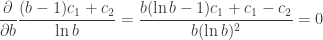
 ,
, .
. and
and  , one axes being


 .
. ths. To express the result correctly in


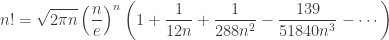
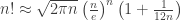
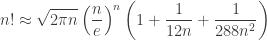
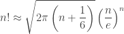
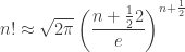
 (and its logarithm) keep showing up in the analysis of algorithm. Unfortunately, it’s very often unwieldy, and we use approximations of
  ) to simplify things. Let’s examine a few!
 ,
,
 ,
, .
. .
. .
. .
. .
.


 into the square root; so it’s a good numerical trade off. However, “Stirling More” and Mohanty & Rummens’ compare with a slight advantage to the later.


 .
.
 to
to  ) (in appropriate luminosity units), others, like Fein and Szuts[
 to
to  ). Depending on the range, that’d yield
 bits,
bits, bits.
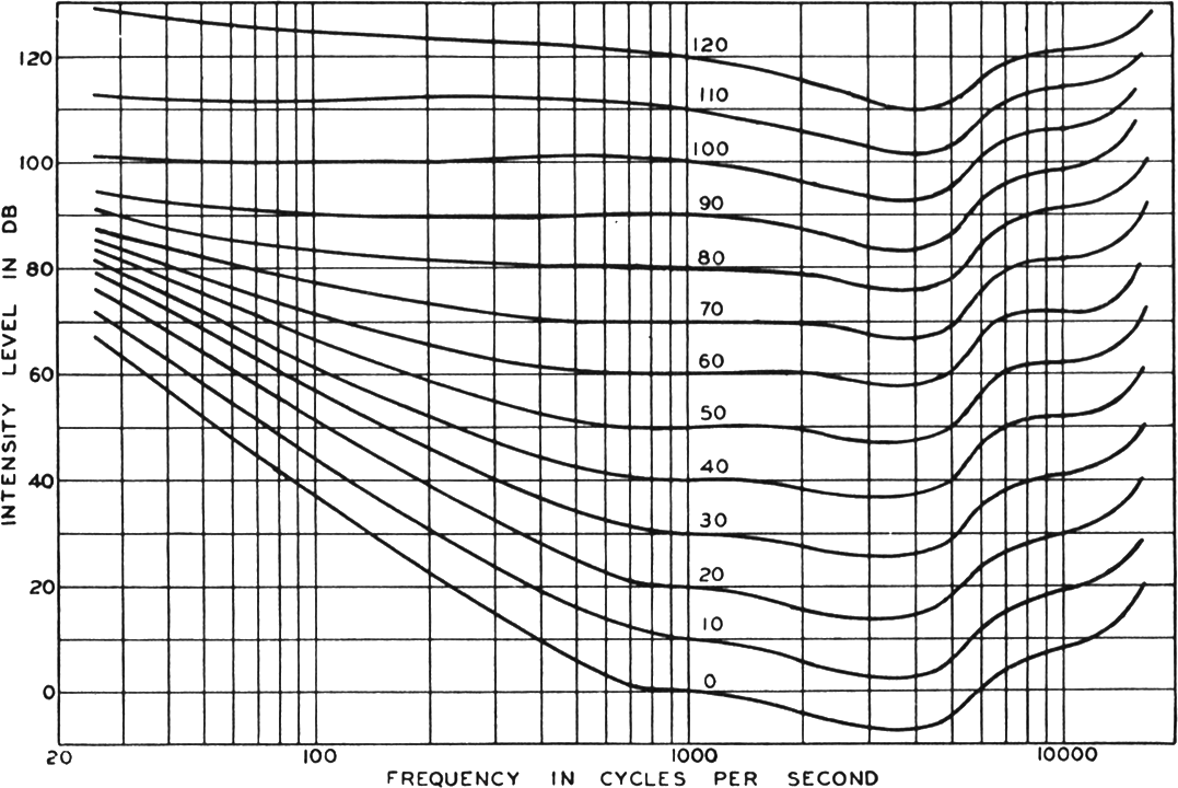
bits. in the figure, only a certain range can be perceived (with lower range marked as
  ). That range seems to be only 4, or 5 order of magnitude, so only
 bits.
bits.


