Annoying Precision — GeistHaus

Qiaochu Yuan Nov 3, 2020

In Part I we discussed some conceptual proofs of the Sylow theorems. Two of those proofs involve reducing the existence of Sylow subgroups to the existence of Sylow subgroups of and respectively. The goal of this post is to understand the Sylow -subgroups of in more detail and see what we can learn from them […]

Show full content

In Part I we discussed some conceptual proofs of the Sylow theorems. Two of those proofs involve reducing the existence of Sylow subgroups to the existence of Sylow subgroups of $S_n$ and $GL_n(\mathbb{F}_p)$ respectively. The goal of this post is to understand the Sylow $p$ -subgroups of $GL_n(\mathbb{F}_p)$ in more detail and see what we can learn from them about Sylow subgroups in general.

Explicit Sylow theory for $GL_n(\mathbb{F}_p)$

Our starting point is the following.

Baby Lie-Kolchin: Let $P$ be a finite $p$ -group acting linearly on a finite-dimensional vector space $V$ over $\mathbb{F}_p$ . Then $P$ fixes a nonzero vector; equivalently, $V$ has a trivial subrepresentation.

Proof. If $\dim V = n$ then there are $p^n - 1$ nonzero vectors in $V \setminus \{ 0 \}$ , so by the PGFPT $P$ fixes at least one of them (in fact at least $p-1$ but these are just given by scalar multiplication). $\Box$

Now we can argue as follows. If $P$ is a finite $p$ -group acting on an $n$ -dimensional vector space $V$ over $\mathbb{F}_p$ (equivalently, up to isomorphism, a finite $p$ -subgroup of $GL_n(\mathbb{F}_p)$ ), it fixes some nonzero vector $v_1 \in V$ . Writing $V_1 = \text{span}(v_1)$ , we get a quotient representation on $V/V_1$ , on which $P$ fixes some nonzero vector, which we lift to a vector $v_2 \in V$ , necessarily linearly independent from $v_1$ , such that $P$ acts upper triangularly on $V_2 = \text{span}(v_1, v_2)$ .

Continuing in this way we get a sequence $v_1, \dots v_n$ of linearly independent vectors (hence a basis of $V$ ) and an increasing sequence $V_k = \text{span}(v_1, \dots v_k)$ of subspaces of $V$ that $P$ leaves invariant, satisfying the additional condition that $P$ fixes $v_k \bmod V_{k-1}$ . The subspaces $V_k$ form a complete flag in $V$ , and writing the elements of $P$ as matrices with respect to the basis $v_1, \dots v_n$ , we see that the conditions that $P$ leaves $V_k$ invariant and fixes $v_k \bmod V_{k-1}$ says exactly that $P$ acts by upper triangular matrices with $1$ s on the diagonal in this basis.

Conjugating back to the standard basis, we’ve proven:

Proposition: Every $p$ -subgroup of $GL_n(\mathbb{F}_p)$ is conjugate to a subgroup of the unipotent subgroup $U_n(\mathbb{F}_p)$ .

This is almost a proof of Sylow I and II for $GL_n(\mathbb{F}_p)$ (albeit at the prime $p$ only), but because we defined Sylow $p$ -subgroups to be $p$ -subgroups having index coprime to $p$ , we’ve only established that $U_n(\mathbb{F}_p)$ is maximal, not that it’s Sylow.

We can show that it’s Sylow by explicitly dividing its order into the order of $GL_n(\mathbb{F}_p)$ but there’s a more conceptual approach that will teach us more. Previously we proved the normalizer criterion: a $p$ -subgroup $P$ of a group $G$ is Sylow iff the quotient $N_G(P)/P$ has no elements of order $p$ .

Claim: The normalizer of $U = U_n(\mathbb{F}_p)$ is the Borel subgroup $B = B_n(\mathbb{F}_p)$ of upper triangular matrices (with no restrictions on the diagonal). The quotient $B/U$ is the torus $(\mathbb{F}_p^{\times})^n$ and in particular has no elements of order $p$ .

Corollary (Explicit Sylow I and II for $GL_n(\mathbb{F}_p)$ : $U_n(\mathbb{F}_p)$ is a Sylow $p$ -subgroup of $GL_n(\mathbb{F}_p)$ .

Proof. The normalizer $N_G(U)$ is the stabilizer of $G = GL_n(\mathbb{F}_p)$ acting on the set of conjugates of $U$ . We want to show that $N_G(U) = B$ , which would mean that the action of $G$ on the conjugates of $U$ can be identified with the quotient $G/B$ .

This quotient is the complete flag variety: it can be identified with the action of $G$ on the set of complete flags in $\mathbb{F}_p^n$ , since the action on flags is transitive and the stabilizer of the standard flag

$\displaystyle 0 \subset \text{span}(e_1) \subset \text{span}(e_1, e_2) \subset \dots \subset \mathbb{F}_p^n$

is exactly $B$ . So it suffices to exhibit a $G$ -equivariant bijection between conjugates of $U$ and complete flags which sends $U$ to the standard flag, since then their stabilizers must agree.

But this is clear: given a complete flag

$\displaystyle 0 = V_0 \subset V_1 \subset \dots \subset V_n = \mathbb{F}_p^n$

we can consider the subgroup of $g \in G$ which preserves the flag (so $g V_i = V_i$ ) and which has the additional property that the induced action on $V_{i+1}/V_i$ is trivial for every $i$ . This produces $U$ when applied to the standard flag, so produces conjugates of $U$ when applied to all flags. In the other direction, given a conjugate $gUg^{-1}$ of $U$ , it has a $1$ -dimensional invariant subspace $V_1$ acting on $\mathbb{F}_p^n$ , quotienting by this subspace produces a unique $1$ -dimensional invariant subspace $V_2/V_1$ acting on $\mathbb{F}_p^n/V_1$ , etc.; this produces the standard flag when applied to $U$ , so produces $g$ applied to the standard flag when applied to conjugates of $U$ . So we get our desired $G$ -equivariant bijection between conjugates of $U$ and complete flags, establishing $N_G(U) = B$ as desired. $\Box$

(This argument works over any field.)

From here it’s not hard to also prove

Explicit Sylow III for $GL_n(\mathbb{F}_p)$ : The number $n_p$ of conjugates of $U_n(\mathbb{F}_p)$ in $GL_n(\mathbb{F}_p)$ divides the order of $GL_n(\mathbb{F}_p)$ and is congruent to $1 \bmod p$ .

Proof. Actually we can compute $n_p$ exactly: we established above that it’s the number of complete flags in $\mathbb{F}_p^n$ (on which $GL_n(\mathbb{F}_p)$ acts transitively, hence the divisibility relation), and a classic counting argument (count the number of possibilities for $V_1$ , then for $V_2$ , etc.) gives the $p$ -factorial

$\displaystyle n_p = [n]_p! = \prod_{i=1}^n [i]_p = \prod_{i=1}^n \left( p^{i-1} + p^{i-2} + \dots + 1 \right)$

which is clearly congruent to $1 \bmod p$ . $\Box$

We could also have done this by dividing the order of $GL_n(\mathbb{F}_p)$ by the order of the Borel subgroup $B$ , but again, doing it this way we learn more, and in fact we get an independent proof of the formula

$\displaystyle |GL_n(\mathbb{F}_p)| = p^{ {n \choose 2} } (p - 1)^n [n]_p!$

for the order of $GL_n(\mathbb{F}_p)$ , where all three factors acquire clear interpretations: the first factor is the order of the unipotent subgroup $U$ , the second factor is the order of the torus $B/U \cong (\mathbb{F}_p^{\times})^n$ , and the third factor is the size of the flag variety $G/B$ .

What is going on in these proofs?

Let’s take a step back and compare these explicit proofs of the Sylow theorems for $GL_n(\mathbb{F}_p)$ to the general proofs of the Sylow theorems. The first three proofs we gave of Sylow I (reduction to $S_n$ , reduction to $GL_n(\mathbb{F}_p)$ , action on subsets) all proceed by finding some clever way to get a finite group $G$ to act on a finite set $X$ with the following two properties:

$|X| \not \equiv 0 \bmod p$ . By the PGFPT this means any $p$ -subgroups of $G$ act on $X$ with fixed points, so we can look for $p$ -subgroups in the stabilizers $\text{Stab}_G(x), x \in X$ .
The stabilizers of the action of $G$ on $X$ are $p$ -groups. Combined with the first property, this means that at least one stabilizer must be a Sylow $p$ -subgroup, since at least one stabilizer must have index coprime to $p$ .

In fact finding a transitive such action is exactly equivalent to finding a Sylow $p$ -subgroup $P$ , since it must then be isomorphic to the action of $G$ on $G/P$ . The nice thing, which we make good use of in the proofs, is that we don’t need to restrict our attention to transitive actions, because the condition that $|X| \not \equiv 0 \bmod p$ has the pleasant property that if it holds for $X$ then it must hold for at least one of the orbits of the action of $G$ on $X$ . (This is a kind of “ $\bmod p$ pigeonhole principle.”)

In the explicit proof for $G = GL_n(\mathbb{F}_p)$ we find $X$ by starting with the action of $G$ on the set of nonzero vectors $\mathbb{F}_p^n \setminus \{ 0 \}$ , which satisfies the first condition but not the second, and repeatedly “extending” the action (to pairs of a nonzero vector $v_1$ and a nonzero vector in the quotient $\mathbb{F}_p^n/v_1$ , etc.) until we arrived at an action satisfying both conditions, namely the action of $G$ on the set of tuples of a nonzero vector $v_1$ , a nonzero vector $v_2 \in \mathbb{F}_p^n/v_1$ , a nonzero vector $v_3 \in \mathbb{F}_p^n / \text{span}(v_1, v_2)$ , etc. (a slightly decorated version of a complete flag).

The next question we’ll address in Part III is: can we do something similar for $G = S_n$ ?

http://qchu.wordpress.com/?p=29026

Extensions

Meditation on the Sylow theorems I

Qiaochu Yuan Nov 1, 2020

As an undergraduate the proofs I saw of the Sylow theorems seemed very complicated and I was totally unable to remember them. The goal of this post is to explain proofs of the Sylow theorems which I am actually able to remember, several of which use our old friend The -group fixed point theorem (PGFPT): If […]

Show full content

The $p$ -group fixed point theorem (PGFPT): If $P$ is a finite $p$ -group and $X$ is a finite set on which $P$ acts, then the subset $X^P$ of fixed points satisfies $|X^P| \equiv |X| \bmod p$ . In particular, if $|X| \not \equiv 0 \bmod p$ then this action has at least one fixed point.

There will be some occasional historical notes taken from Waterhouse’s The Early Proofs of Sylow’s Theorem.

A quick note on the definition of a Sylow subgroup

A Sylow $p$ -subgroup of a finite group $G$ can be equivalently defined as either a $p$ -subgroup of index coprime to $|G|$ (that is, if $|G| = p^n k$ where $\gcd(p, k) = 1$ , then $|P| = p^n$ ) or a $p$ -subgroup which is maximal with respect to inclusion. The equivalence of these two definitions requires the Sylow theorems, but we’ll want to discuss such subgroups before proving them, and for the purposes of this post it will be most convenient to adopt the first definition.

So for the rest of this post, a Sylow $p$ -subgroup is a $p$ -subgroup of index coprime to $p$ , and we’ll refer to $p$ -subgroups maximal with respect to inclusion as maximal $p$ -subgroups before we prove that the two are equivalent.

Warmup: Cauchy’s theorem

We’ll start off by giving some proofs of Cauchy’s theorem. One of the proofs of Sylow I later needs it as a lemma, and some of the proofs we give here will generalize to proofs of Sylow I. First we quote the proof using the PGFPT in full from the above blog post, as Proof 1.

Cauchy’s theorem: Let $G$ be a finite group. Suppose $p$ is a prime dividing $|G|$ . Then $G$ has an element of order $p$ .

Proof 1 (PGFPT). $\mathbb{Z}/p\mathbb{Z}$ acts by cyclic shifts on the set

$\{ (g_1, g_2, ... g_p) \in G^p : g_1 g_2 ... g_p = 1 \} \setminus \{ (1, 1, ... 1) \in G^p \}$

since if $g_1 g_2 ... g_p = 1$ then $g_p (g_1 g_2 ... g_p) g_p^{-1} = 1$ . This set has cardinality $|G|^{p-1} - 1$ , which is not divisible by $p$ , hence $\mathbb{Z}/p\mathbb{Z}$ has a fixed point, which is precisely a nontrivial element $g \in G$ such that $g^p = 1$ . $\Box$

This proof is almost disgustingly short. By contrast, according to Waterhouse, Cauchy’s original proof runs nine pages (!) and works as follows.

First Cauchy explicitly constructs Sylow $p$ -subgroups of the symmetric group $S_n$ . This can be done by recursively partitioning $\{ 1, 2, \dots n \}$ into $\lfloor \frac{n}{p} \rfloor$ blocks of size $p$ , considering the subgroup generated by $p$ -cycles cyclically permuting each block, then partitioning the set of blocks itself into $\lfloor \frac{n}{p^2} \rfloor$ blocks-of-blocks of size $p$ , cyclically permuting these, and so forth. This subgroup has size

$\displaystyle p^{ \sum_{k \ge 1} \left\lfloor \frac{n}{p^k} \right\rfloor }$

and the exponent is Legendre’s formula for the largest power $\nu_p(n!)$ of $p$ dividing $|S_n|$ . It follows that this is a Sylow $p$ -subgroup.

Second, Cauchy proves a special case of the following lemma, namely the special case that $H = S_n$ . This lemma doesn’t appear to have a standard name, so we’ll name it

Cauchy’s $p$ -group lemma: Let $G$ be a subgroup of a finite group $H$ such that $H$ has a Sylow $p$ -subgroup $P$ . If $p \mid |G|$ , then $G$ has an element of order $p$ .

Proof. We’ll prove the contrapositive: if $G$ doesn’t contain an element of order $p$ , then $p$ does not divide $|G|$ .

Consider the left action of $G$ on the set of cosets $H/P$ . By grouping the cosets into $G$ -orbits and using the orbit-stabilizer theorem we have

$\displaystyle |H/P| = \sum_{[h] \in G \backslash H/P} \frac{|G|}{|\text{Stab}_G(hP)|}$

where $G \backslash H/P$ is the collection of double cosets and the stabilizer of a coset is

$\displaystyle \text{Stab}_G(hP) = \{ g \in G : ghP = hP \} = \{ g \in G : h^{-1} gh \in P \} = h^{-1} G h \cap P$

and in particular it has order dividing $|P|$ , hence a power of $p$ .

If $G$ has no element of order $p$ , then since any nontrivial subgroup of $P$ contains an element of order $p$ , these stabilizers are all trivial, so we get that

$\displaystyle |H/P| = |G| |G \backslash H/P|$

and in particular that $|G|$ divides $|H/P|$ . Since $P$ is a Sylow $p$ -subgroup, $|H/P|$ isn’t divisible by $p$ , and hence neither is $|G|$ . $\Box$

Call a collection of finite groups cofinal if every finite group embeds into at least one of them.

Corollary: To prove Cauchy’s theorem for all finite groups, it suffices to find a cofinal collection of finite groups which have Sylow $p$ -subgroups.

We can now complete Cauchy’s proof of Cauchy’s theorem.

Proof 2 (symmetric groups). The symmetric groups $\{ S_n \}$ are cofinal (this is exactly Cayley’s theorem) and have Sylow $p$ -subgroups. $\Box$

But we don’t have to use the symmetric groups!

Proof 3 (general linear groups). Since the symmetric groups $S_n$ embed into the general linear groups $GL_n(\mathbb{F}_p)$ , the latter are also cofinal, and we can also exhibit Sylow $p$ -subgroups for them: the unipotent subgroup $U_n(\mathbb{F}_p)$ of upper triangular matrices with $1$ s on the diagonal is Sylow. This follows from the standard calculation of the order

$\displaystyle |GL_n(\mathbb{F}_p)| = p^{ {n \choose 2} } (p-1)^n [n]_p!$

where $[n]_p!$ is the $p$ -factorial. $\Box$

Here’s a fourth proof that doesn’t use Cauchy’s lemma and doesn’t require the clever construction of the first proof; Waterhouse says it’s used by Rotman.

Proof 4 (class equation). We induct on the order of $G$ . First we observe that Cauchy’s theorem is straightforwardly true for finite abelian groups by using the Chinese remainder theorem to write a finite abelian group as a direct sum of finite abelian $p$ -groups. (And then, to spell it out very explicitly, Lagrange’s theorem implies that any nontrivial element of a finite $p$ -group has $p$ -power order, so some power of that element has order $p$ .)

Next, given a finite group $G$ such that $p \mid |G|$ we consider the class equation

$\displaystyle |G| = |Z(G)| + \sum_i \frac{|G|}{|C_G(g_i)|}$

where the sum runs over non-central conjugacy classes. If $p \mid |Z(G)|$ then we’re done by reduction to the abelian case. Otherwise, $p$ doesn’t divide $|Z(G)|$ but does divide $|G|$ , so by taking both sides $\bmod p$ we conclude that there is some $g_i$ such that the centralizer $C_G(g_i)$ has index in $G$ coprime to $p$ , and hence $p \mid |C_G(g_i)|$ . Since $g_i$ is a non-central conjugacy class $C_G(g_i)$ has order strictly less than $|G|$ so has an element of order $p$ by the inductive hypothesis. $\Box$

Sylow I

With very little additional effort the above proof of Cauchy’s $p$ -group lemma actually proves the following stronger result; Waterhouse attributes this argument, again in the special case that $H = S_n$ , to Frobenius. It also doesn’t appear to have a standard name, so we’ll call it

Frobenius’ $p$ -group lemma: Let $G$ be a subgroup of a finite group $H$ such that $H$ has a Sylow $p$ -subgroup $P$ . Then $G$ also has a Sylow $p$ -subgroup, given by its intersection with some conjugate of $P$ .

Proof. Consider as before the sum

$\displaystyle |H/P| = \sum_{[h] \in G \backslash H/P} \frac{|G|}{|h^{-1} G h \cap P|}$

obtained by considering the orbits of the action of $G$ on $H/P$ . Since $p$ doesn’t divide $|H/P|$ , at least one term on the RHS is also not divisible by $p$ , so there exists some $h$ such that $h^{-1} G h \cap P$ has index coprime to $p$ and hence is a Sylow $p$ -subgroup of $h^{-1} G h$ ; conjugating, we get that the intersection of $h P h^{-1}$ with $G$ is a Sylow $p$ -subgroup of $G$ as desired. $\Box$

Corollary: To prove that Sylow subgroups exist for all finite groups, it suffices to prove that they exist for a cofinal collection of finite groups.

Now we can give two different proofs of Sylow I, as follows.

Sylow I: Every finite group $G$ has a Sylow $p$ -subgroup.

(Note that with our definitions if $\gcd(p, |G|) = 1$ then this subgroup is just the trivial group.)

Proof 1 (symmetric groups). It suffices to prove the existence of Sylow subgroups for the symmetric groups $S_n$ , which was done above. $\Box$

Proof 2 (general linear groups). It suffices to prove the existence of Sylow $p$ -subgroups for $GL_n(\mathbb{F}_p)$ , which was done above. Running the argument gives that every finite $p$ -group is a subgroup of $U_n(\mathbb{F}_p)$ for some $n$ , which gives an independent proof that finite $p$ -groups are nilpotent. $\Box$

Proof 2 is the first proof of Sylow I given by Serre in his Finite Groups: An Introduction.

I heard a rumor years ago that these proofs existed but didn’t see them; glad that’s finally settled.

The next proof of Sylow I we’ll present is the one that I saw as an undergraduate, in Artin’s Algebra if memory serves. According to Wikipedia it’s due to Wielandt. Serre attributes it to “Miller-Wielandt” and it’s the second proof he gives.

Proof 3 (action on subsets). Write $|G| = p^k m$ where $\gcd(p, m) = 1$ and consider the action of $G$ by left multiplication on the set ${G \choose p^k}$ of $p^k$ -element subsets of $G$ . We’ll show that there exists a stabilizer subgroup of size $p^k$ .

(I found this construction very bizarre and unmotivated as an undergraduate. I like it better now, I guess, but I’m still a little mystified.)

Key observation: An element $g \in G$ stabilizes a subset $S \subseteq G$ iff $S$ consists of cosets of the cyclic subgroup $\langle g \rangle$ generated by $g$ ; in particular a necessary condition is that its order must divide the size of $S$ .

This means that the action of $G$ on ${G \choose p^k}$ has the property that all stabilizers must be $p$ -groups (just like the action of $G$ on $H/P$ we used above). As before, decomposing this action into orbits gives

$\displaystyle {|G| \choose p^k} = \sum_{[S]} \frac{|G|}{|\text{Stab}(S)|}$

where the sum runs over a set of orbit representatives.

Lemma: $\displaystyle {p^k m \choose p^k} \ \equiv m \bmod p$ .

Proof. This is a special case of Lucas’ theorem , which we proved using the PGFPT previously. $\Box$

It follows that ${|G| \choose p^k} \equiv m \bmod p$ is not divisible by $p$ , so there exists some subset $S$ such that $\frac{|G|}{|\text{Stab}(S)|}$ is also not divisible by $p$ . But since $|\text{Stab}(S)|$ is a power of $p$ this is only possible if $|\text{Stab}(S)| = p^k$ . This stabilizer is a Sylow $p$ -subgroup as desired. $\Box$

This proof is tantalizingly similar to the proof of Frobenius’ lemma above; in both cases the key is to write down an action of $G$ on a set of size relatively prime to $p$ but such that all stabilizers must be $p$ -groups. But I’m not yet sure how to relate them.

We’re not done with proofs of Sylow I! The next proof is due to Frobenius; Waterhouse stresses that its early use of quotients crucially highlighted the importance of working with abstract groups rather than just groups of substitutions as was standard in early group theory. It generalizes the class equation proof of Cauchy’s theorem above.

Proof 4 (class equation). We again induct on the order of $|G|$ and start by observing that Sylow subgroups clearly exist for finite abelian groups, for example by the structure theorem. We can also use the Chinese remainder theorem.

Now, suppose that $p \mid |G|$ . If $p$ also divides the order $|Z(G)|$ of the center, then $Z(G)$ contains a (central, abelian, nontrivial) Sylow $p$ -subgroup $A$ , which we can quotient by. Then $G/A$ , by the inductive hypothesis, also contains a Sylow $p$ -subgroup, and the preimage of this subgroup is a Sylow $p$ -subgroup of $G$ .

If $p \nmid |Z(G)|$ , then again we inspect the class equation

$\displaystyle |G| = |Z(G)| + \sum_i \frac{|G|}{|C_G(g_i)|}$

where again the sum runs over non-central conjugacy classes. Since $p \mid |G|$ we conclude that there is some conjugacy class $[g_i]$ such that $p \nmid \frac{|G|}{|C_G(g_i)|}$ , hence such that $|G|$ and $|C_G(g_i)|$ have the same $p$ -adic valuation. By the inductive hypothesis, $C_G(g_i)$ contains a Sylow $p$ -subgroup, which is then (by virtue of having the appropriate order) also a Sylow $p$ -subgroup of $G$ . $\Box$

This proof is the first one we’ve seen that provides a halfway reasonable algorithm for finding Sylow subgroups, which is lovely (the first three are more or less just raw existence proofs): pass to the quotient by central $p$ -groups until you can’t anymore, then search for conjugacy classes whose centralizers have index relatively prime to $p$ and pass to the centralizers until you can’t anymore, then repeat.

We give one final proof. According to Waterhouse, this one is essentially Sylow’s original proof, and it naturally proves an apparently-slightly-stronger result, interpolating between Cauchy’s theorem and Sylow I. It also provides a (different) algorithm for finding Sylow subgroups.

Sylow I+: Every finite group $G$ contains a subgroup of prime power order $p^k$ whenever $p^k \mid |G|$ . These subgroups can be constructed inductively by starting from an element of order $p$ and then finding an element of $p$ -power order normalizing the previous subgroup.

(Note that this result is equivalent to Sylow I as usually stated once we know that finite $p$ -groups admit composition series in which each quotient is $C_p$ , which is not hard to prove by induction once we know that finite $p$ -groups have nontrivial center, which in turn we proved previously using the PGFPT. The below proof actually gives an independent proof of the existence of such a composition series, and hence an independent proof that finite $p$ -groups are nilpotent.)

Proof 5 (normalizers + PGFPT). We induct on $k$ . The base case $k = 1$ is Cauchy’s theorem, which we proved above (four times!).

Now suppose we’ve found a subgroup $P$ of order $p^k$ , and we’d like to see if we can find a subgroup of order $p^{k+1}$ . Consider the action of $P$ by left multiplication on the cosets $G/P$ . By the PGFPT the number of fixed points of this action satisfies

$\displaystyle |(G/P)^P| \equiv |G/P| \bmod p$ .

On the other hand, the fixed points of this action are precisely the cosets $gP$ such that $PgP = gP$ , or equivalently such that $g^{-1} P g = P$ . So they are naturally in bijection with the quotient $N_G(P)/P$ of the normalizer

$\displaystyle N_G(P) = \{ g \in G : gPg^{-1} = P \}$

of $P$ . So the PGFPT tells us:

Lemma: If $P$ is a $p$ -subgroup of a finite group $G$ , then $|G/P| \equiv |N_G(P)/P| \bmod p$ .

If $p^{k+1} \mid |G|$ , or equivalently if $P$ is not a Sylow $p$ -subgroup, then $|G/P| \equiv 0 \bmod p$ and hence $|N_G(P)/P| \equiv 0 \bmod p$ , so by Cauchy’s theorem it follows that $N_G(P)/P$ has an element $g$ of order $p$ . The preimage of the cyclic subgroup $\langle g \rangle$ in $N_G(P)$ is then a $p$ -subgroup of order $p^{k+1}$ as desired; more specifically it’s a subgroup $P'$ given by some extension

$\displaystyle 1 \to P \to P' \to C_p \to 1$

where $g$ generates the copy of $C_p$ . So we’ve found our bigger $p$ -subgroup. $\Box$

This proof gives us an algorithm for finding Sylow subgroups by starting with elements of order $p$ and repeatedly finding elements of order $p^k$ in the normalizer, and note that it also gives us a way to prove that a $p$ -subgroup is Sylow without explicitly checking that its index is coprime to $p$ :

Corollary (normalizer criterion): A $p$ -subgroup $P$ of a finite group $G$ is a Sylow $p$ -subgroup iff the quotient $N_G(P)/P$ contains no elements of order $p$ .

It has another corollary we haven’t quite gotten around to proving yet:

Corollary (Sylow = maximal): Sylow $p$ -subgroups are precisely the maximal $p$ -subgroups.

(Before it could have been the case that there were $p$ -subgroups maximal with respect to inclusion but without index coprime to $p$ .)

These are all the proofs of Sylow I that I know or could track down. After having gone through all of them I think I like proof 4 (class equation) and proof 5 (normalizers) the best. Proof 3 (action on subsets) is really too opaque and too specialized; you only learn from it that Sylow subgroups exist and practically nothing else, whereas proof 4 and proof 5 both teach you more about them, including how to find them. I’m sort of amazed it took me over 10 years after I first ran into the Sylow theorems to finally see a version of Sylow’s original proof, and that when I did, I liked it so much better than the first proof I had seen.

Sylow II and III

These will be short.

Sylow II: Let $G$ be a finite group and $P$ be any Sylow $p$ -subgroup. Every $p$ -subgroup $K$ of $G$ is contained in a conjugate of $P$ . In particular, taking $K$ to be another Sylow $p$ -subgroup, every pair of Sylow $p$ -subgroups is conjugate.

Proof 1. Immediate corollary of Frobenius’ lemma. $\Box$

Proof 2. Consider the action of $K$ on $G/P$ . By hypothesis, $|G/P| \not \equiv 0 \bmod p$ , so by the PGFPT,

$\displaystyle |(G/P)^K| \equiv |G/P| \not \equiv 0 \bmod p$ .

A fixed point of the action of $K$ on $G/P$ is precisely a coset $gP$ such that $KgP = gP$ , or equivalently such that $g^{-1} K g \subseteq P$ , so there must be at least one such $g$ conjugating $K$ into $P$ as desired. $\Box$

Corollary (Sylow = maximal, again): Sylow $p$ -subgroups are precisely the maximal $p$ -subgroups.

(We’ve now proved this result in three different ways!)

Sylow III: Let $G$ be a finite group and $P$ be any Sylow $p$ -subgroup. The number $n_p$ of Sylow $p$ -subgroups of $G$ satisfies $n_p = |G/N_G(P)|$ and $n_p \equiv 1 \bmod p$ ; in particular, $n_p \mid |G|$ .

Proof. Since the Sylow $p$ -subgroups are conjugate, the set of Sylow $p$ -subgroups is just the set of conjugates of $P$ . $G$ acts transitively on this set by conjugation with stabilizer $N_G(P)$ , so by orbit-stabilizer it has size $n_p = |G/N_G(P)|$ and in particular has size dividing $|G|$ . We now give two proofs of the all-important congruence $n_p \equiv 1 \bmod p$ .

Subproof 1 (action of $P$ on $G/P$ ). In Proof 5 (normalizers + PGFPT) of Sylow I above we showed that

$\displaystyle |G/P| \equiv |N_G(P)/P| \not \equiv 0 \bmod p$

and dividing both sides by $|N_G(P)/P| \bmod p$ gives the desired result.

Subproof 2 (action of $P$ on $G/N_G(P)$ ). This proof has the benefit of explaining what this congruence “means.” $N_G(P)/P$ can’t be divisible by $p$ , so the only elements of $p$ -power order that normalize $P$ are the elements of $P$ , and the same must be true for any other Sylow. This implies that if we restrict the conjugation action of $G$ on the Sylows to $P$ , then $P$ fixes only itself, so by the PGFPT

$\displaystyle |(G/N_G(P))^P| = 1 \equiv |G/N_G(P)| = n_p \bmod p$

and the conclusion follows. $\Box$

http://qchu.wordpress.com/?p=28470

Extensions

Compression and Kolmogorov complexity

Qiaochu Yuan Sep 27, 2020

This is a post I wanted to write some time ago; I’ve forgotten why, but it was short and cute enough to finish. Our starting point is the following observation: Theorem 1: Universal lossless compression is impossible. That is, there is no function which takes as input finite strings (over some fixed alphabet) and always […]

Show full content

This is a post I wanted to write some time ago; I’ve forgotten why, but it was short and cute enough to finish. Our starting point is the following observation:

Theorem 1: Universal lossless compression is impossible. That is, there is no function which takes as input finite strings (over some fixed alphabet) and always produces as output shorter finite strings (over the same alphabet) in such a way that the latter is recoverable from the former.

Supposedly people sometimes claim to be able to do this. It is as impossible as constructing a perpetual motion machine, if not more so, and for much more easily understandable reasons.

Proof. The problem is simply that there are not enough short strings. To be specific, let’s work with just binary strings. There are $2^n$ strings of length $n$ , and

$\displaystyle 1 + 2 + 2^2 + \dots + 2^{n-1} = 2^n - 1$

strings of length at most $n-1$ , which is smaller. Hence there’s no injective function from the set of binary strings of length $n$ to the set of binary strings of length at most $n-1$ , for any $n$ . The problem only gets worse if $2$ is replaced by a larger number, or if we try to compress strings of length at most $n$ instead of strings of length exactly $n$ . $\Box$

Informally, another way to summarize the argument is that it takes $n$ bits to represent an arbitrary binary string of length $n$ , and less than $n$ bits to represent an arbitrary binary string of length at most $n-1$ .

This argument straightforwardly implies that any lossless compression algorithm which makes at least one of its inputs smaller necessarily makes at least one of its inputs larger, and more broadly draws attention to the set of inputs one might actually want to compress in practice. If you want to compress 1000×1000 images – strings of a million pixels – but you only want to compress, say, photos that humans might actually take, this is potentially much smaller than the set of all 1000×1000 images (for example, because most real images have the property that most of the time, a pixel is close in color to its neighbors), and so the theoretical lower bound on how well such images can be compressed might be much better.

More generally, the situation is improved if you have a probability distribution over inputs you want to compress with low entropy and you only want to compress well on average, which allows you to do something like Huffman coding. (This is a generalization because the uniform distribution over a set of size $N$ has entropy $\log_2 N$ .) Probably all probability distributions describing real-life data have this property. And this is before taking into account the possibility of lossy compression.

What I like about Theorem 1 is that it is both incredibly easy to prove and a surprisingly deep and important fact. Here is, for example, another very important result that is arguably just a corollary of Theorem 1.

Consider what is in some sense the “ultimate” lossless compression scheme, namely, given a binary string of length $n$ , compress it to the shortest program, in some fixed programming language, which prints that string. The length of this program – let’s also write it as a binary string, using ASCII or equivalent – is called the Kolmogorov complexity of the string. Let’s call this Kolmogorov compression.

The sense in which Kolmogorov compression is the “ultimate” lossless compression scheme is that whatever decompression is, it surely ought to be computable or else we wouldn’t be able to do it (ignoring for the moment that Kolmogorov compression is uncomputable!), and any compression scheme whatsoever (computable or not) which compresses some complicated input string $X$ into a string of length $\ell$ , together with the decompression program, constitutes a program which prints $X$ , of size at most $\ell$ plus the size of the decompression program, which is a constant.

So the Kolmogorov complexity of a string is a lower bound, up to an additive constant, on the length of a string that compresses it, according to any compression scheme with a computable decompression function. (Of course you can come up with a silly compression scheme which “memorizes” any fixed string and compresses it arbitrarily small, but the price you pay is that the Kolmogorov complexity of this string is more or less a lower bound on the size of your decompression program, and also there’s no reason this would help you compress anything you actually care about.)

Now, Theorem 1, applied to Kolmogorov compression, implies the following.

Theorem 2: For every $n$ , there exist strings of length $n$ whose Kolmogorov complexity is at least $n$ .

In other words, there exist incompressible strings, whose shortest descriptions are just those strings themselves. In fact, most strings are basically incompressible in this sense; a slight generalization of Theorem 1 shows that at most $\frac{1}{2^k}$ of all binary strings of length $n$ can be compressed to have length at most $n-k-1$ . For example, taking $k = 7$ , less than 1% of strings of length $n \ge 8$ can have their length reduced by $8$ or more by any fixed compression scheme.

This observation suggests an important connection between incompressibility and randomness. On the one hand, a randomly chosen string is incompressible with high probability. On the other hand, incompressible strings “look random” – they don’t have any patterns in them, because patterns can be described by short programs.

http://qchu.wordpress.com/?p=28086

Extensions

Gradient descent

Qiaochu Yuan Feb 7, 2018

Note: this is a repost of a Facebook status I wrote off the cuff about a year ago, lightly edited. As such it has a different style from my other posts, but I still wanted to put it somewhere where it’d be easier to find and share than Facebook. Gradient descent, in its simplest where […]

Show full content

Gradient descent, in its simplest where you just subtract the gradient of your loss function $J$ , is not dimensionally consistent: if the parameters you’re optimizing over have units of length, and the loss function is dimensionless, then the derivatives you’re subtracting have units of inverse length.

This observation can be used to reinvent the learning rate, which, for dimensional consistency, must have units of length squared. It also suggests that the learning rate ought to be set to something like $L^2$ for some kind of characteristic length scale $L$ , which loosely speaking is the length at which the curvature of $J$ starts to matter.

It might also make sense to give different parameters different units, which suggests furthermore that one might want a different learning rate for each parameter, or at least that one might want to partition the parameters into different subsets and choose different learning rates for each.

Going much further, from an abstract coordinate-free point of view the extra information you need to compute the gradient of a smooth function is a choice of (pseudo-)Riemannian metric on parameter space, which if you like is a gigantic hyperparameter you can try to optimize. Concretely this amounts to a version of preconditioned gradient descent where you allow yourself to multiply the gradient (in the coordinate-dependent sense) by a symmetric (invertible, ideally positive definite) matrix which is allowed to depend on the parameters. In the first paragraph this matrix was a constant scalar multiple of identity and in the third paragraph this matrix was constant diagonal.

This is an extremely general form of gradient descent, general enough to be equivariant under arbitrary smooth change of coordinates: that is, if you do this form of gradient descent and then apply a diffeomorphism to parameter space, you are still doing this form of gradient descent, with a different metric. For example, if you pick the preconditioning matrix to be the inverse Hessian (in the usual sense, assuming it’s invertible), you recover Newton’s method. This corresponds to choosing the metric at each point to be given by the Hessian (in the usual sense), which is the choice that makes the Hessian (in the coordinate-free sense) equal to the identity. This is a precise version of “the length at which the curvature of $J$ starts to matter” and in principle ameliorates the problem where gradient descent performs poorly in narrow valleys (regions where the Hessian (in the usual sense) is poorly conditioned), at least up to cubic and higher order effects.

In general it’s expensive to compute the inverse Hessian, so a more practical thing to do is to use a matrix which approximates it in some sense. And now we’re well on the way towards quasi-Newton methods.

http://qchu.wordpress.com/?p=28434

Extensions

The representation theory of the additive group scheme

Qiaochu Yuan Nov 27, 2017

In this post we’ll describe the representation theory of the additive group scheme over a field . The answer turns out to depend dramatically on whether or not has characteristic zero. Preliminaries over an arbitrary ring (All rings and algebras are commutative unless otherwise stated.) The additive group scheme over a base ring has functor of […]

Show full content

In this post we’ll describe the representation theory of the additive group scheme $\mathbb{G}_a$ over a field $k$ . The answer turns out to depend dramatically on whether or not $k$ has characteristic zero.

Preliminaries over an arbitrary ring

(All rings and algebras are commutative unless otherwise stated.)

The additive group scheme $\mathbb{G}_a$ over a base ring $k$ has functor of points given by the underlying abelian group functor

$\displaystyle \mathbb{G}_a(-) : \text{CAlg}(k) \ni R \mapsto (R, +) \in \text{Ab}.$

This functor is represented by the free $k$ -algebra $k[x]$ together with the Hopf algebra structure given by the comultiplication

$\displaystyle \Delta(x) = x \otimes 1 + 1 \otimes x$

and antipode $S(x) = -x$ , and so it is an affine group scheme whose underlying scheme is the affine line $\mathbb{A}^1$ over $k$ . From a Hopf algebra perspective, this Hopf algebra is special because it is the free Hopf algebra on a primitive element.

A representation of $\mathbb{G}_a$ can be described in a few equivalent ways. From the functor of points perspective, we first need to describe the functor of points perspective on a $k$ -module: a $k$ -module $V$ has functor of points

$\displaystyle V(-) : \text{CAlg}(k) \ni R \mapsto R \otimes_k V \in \text{Ab}$

making it an affine group scheme if $V$ is finitely generated projective (in which case its ring of functions is the symmetric algebra $S(V^{\ast})$ on the dual of $V$ ) but not in general, for example if $k$ is a field and $V$ is an infinite-dimensional vector space. Note that if $V = k$ we recover $\mathbb{G}_a$ , and more generally if $V = k^n$ we recover $\mathbb{G}_a^n$ .

A representation of $\mathbb{G}_a$ over $k$ is, loosely speaking, a polynomial one-parameter group of automorphisms of a $k$ -module. The simplest nontrivial example is

$\mathbb{G}_a \ni x \mapsto \left[ \begin{array}{cc} 1 & x \\ 0 & 1 \end{array} \right]$

which defines a nontrivial action of $\mathbb{G}_a$ on $k^2$ .

Formally, we can define an action of $\mathbb{G}_a$ on a $k$ -module $V$ as an action of the functor of points of the former on the functor of points of the latter which is linear in the appropriate sense. Explicitly, it is a natural transformation with components

$\displaystyle \eta_R : \mathbb{G}_a(R) \times V(R) \to V(R)$

such that each $\eta_R$ defines an $R$ -linear action of the group $\mathbb{G}_a(R) \cong (R, +)$ on the $R$ -module $V(R) \cong R \otimes_k V$ in a way which is natural in $R$ . So we can think of the parameter $x$ in the one-parameter group above as running over all elements of all $k$ -algebras $R$ .

$\eta$ can equivalently, by currying, be thought of as a natural transformation of group-valued functors from $\mathbb{G}_a$ to the functor

$\displaystyle \text{Aut}(V)(-) : \text{CAlg}(k) \ni R \mapsto \text{Aut}_R(V \otimes_k R)$

even though the latter is generally not representable by a scheme, again unless $V$ is finitely generated projective; note that if $V = k^n$ then $\text{Aut}(V)$ is an affine group scheme, namely the general linear group $GL_n$ .

The advantage of doing this is that we can appeal to the Yoneda lemma: because $\mathbb{G}_a$ is representable, such natural transformations correspond to elements of the group

$\text{Aut}_{k[x]}(V \otimes_k k[x]) \subseteq \text{End}_{k[x]}(V \otimes_k k[x]) \cong \text{Hom}_k(V, V \otimes_k k[x])$

at which point we’ve finally been freed of the burden of having to consider arbitrary $R$ . Writing down the conditions required for a map $V \to V \otimes_k k[x]$ to correspond to an element of $\text{Aut}_{k[x]}(V(k[x]))$ giving a homomorphism of group-valued functors $\mathbb{G}_a \to \text{Aut}(V)$ , we are led to the following.

Definition-Theorem: A representation of $\mathbb{G}_a$ over $k$ is a comodule over the Hopf algebra of functions $\mathcal{O}_{\mathbb{G}_a} \cong k[x]$ .

This is true more generally for representations of any affine group scheme.

Let’s get somewhat more explicit. A comodule over $k[x]$ is in particular an action map $\alpha : V \to V \otimes_k k[x]$ . Isolating the coefficient of $x^n$ on the RHS, this map breaks up into homogeneous components

$\displaystyle \alpha_n : V \to V \otimes_k x^n$

which each correspond to an element of $\text{End}_k(V)$ , which we’ll call $M_n$ . The entire action map can therefore be thought of as a power series

$\displaystyle M(x) = M_0 + M_1 x + M_2 x^2 + \dots$

and the condition that $\alpha$ is part of a comodule structure turns out to be precisely the condition that 1) $M(0) = M_0$ is the identity, 2) that we have

$\displaystyle M(x + y) = M(x) M(y)$

as an identity of formal power series, and 3) that for any $v \in V$ , $M_i v = 0$ for all but finitely many $i$ . Which of these is nonzero can be read off from the value of $\alpha(v)$ , which takes the form

$\displaystyle \alpha(v) = M(x)(v) = \sum_{i \ge 0} M_i v \otimes x^i$ .

Equating the coefficients of $x^i y^j$ and of $x^j y^i$ on both sides of the identity $M(x + y) = M(x) M(y)$ (the two coefficients are equal on the LHS, hence must be equal on the RHS) gives

$\displaystyle {i + j \choose i} M_{i+j} = M_i M_j = M_j M_i$

from which it follows in particular that the $M_i$ commute. This is necessary and sufficient for us to have $M(x + y) = M(x) M(y)$ , so we can say the following over an arbitrary $k$ :

Theorem: Over a ring $k$ , representations of $\mathbb{G}_a$ can be identified with modules $V$ over the divided power algebra

$\displaystyle k[M_1, M_2, \dots] / \left( {i + j \choose i} M_{i + j} = M_i M_j \right)$

which are locally finite in the sense that for any $v \in V$ we have $M_i v = 0$ for all but finitely many $i$ . Given the action of each $M_i$ , the corresponding action of $\mathbb{G}_a$ is

$\displaystyle \sum_i M_i x^i : V \mapsto V \otimes_k k[x]$ .

If $k$ is torsion-free as an abelian group, for example if $k = \mathbb{Z}$ , then the divided power algebra can be thought of as the subalgebra of $(k \otimes \mathbb{Q})[x]$ spanned by $\frac{x^i}{i!}$ , where the isomorphism sends $M_i$ to $\frac{x^i}{i!}$ . This is because the key defining relation above can be rewritten $(i + j)! M_{i + j} = (i! M_i) (j! M_j)$ if there is no torsion.

These representations should really be thought of as continuous representations of the profinite Hopf algebra given as the cofiltered limit over the algebras spanned by $M_1, M_2, \dots M_n$ for each $n$ , with the quotient maps given by setting all $M_i$ past a certain point to zero. This profinite Hopf algebra is dual to the Hopf algebra $k[x]$ of functions on $\mathbb{G}_a$ , and we can more generally relate comodules over a coalgebra $C$ to modules over a profinite algebra dual to it in this way under suitable hypotheses, for example if $k$ is a field.

In characteristic zero

If $k$ is a field of characteristic zero, or more generally a $\mathbb{Q}$ -algebra, then the divided power algebra simplifies drastically, because we can now divide by all the factorials running around. Induction on the relation ${i + j \choose i} M_{i + j} = M_i M_j$ readily gives

$\displaystyle M_i = \frac{M_1^i}{i!}$

and we conclude the following.

Theorem: Over a $\mathbb{Q}$ -algebra $k$ , representations of $\mathbb{G}_a$ can be identified with endomorphisms $M_1 : V \to V$ of a $k$ -module which are locally nilpotent in the sense that, for any $v \in V$ , we have $M_1^i v = 0$ for all but finitely many $i$ . Given such an endomorphism, the corresponding action of $\mathbb{G}_a$ is

$\displaystyle \exp (M_1 x) : V \to V \otimes_k k[x]$ .

The corresponding profinite Hopf algebra is the formal power series algebra $k[[\partial]]$ in one variable, with comultiplication $\Delta(\partial) = \partial \otimes 1 + 1 \otimes \partial$ . If $k$ is a field of characteristic zero, this means we can at least classify finite-dimensional representations of $\mathbb{G}_a$ using nilpotent Jordan blocks.

Example. The representation $\left[ \begin{array}{cc} 1 & x \\ 0 & 1 \end{array} \right]$ we wrote down earlier corresponds to exponentiating the Jordan block $\left[ \begin{array}{cc} 0 & 1 \\ 0 & 0 \end{array} \right]$ .

Example. Any coalgebra has a “regular representation,” namely the comodule given by its own comultiplication. The regular representation of $\mathbb{G}_a$ is the translation map

$\displaystyle \mathbb{G}_a \ni x \mapsto (f(y) \mapsto f(y+x)) \in \text{Hom}_k(k[y], k[y] \otimes_k k[x])$ .

and the corresponding locally nilpotent endomorphism is the derivative $f \mapsto \partial f$ (hence the use of $\partial$ above). More generally, locally nilpotent derivations on a $k$ -algebra $R$ correspond to actions of $\mathbb{G}_a$ on the affine $k$ -scheme $\text{Spec } R$ .

The regular representation has subrepresentations given by restricting attention to the polynomials of degree at most $n$ for each $n$ . These subrepresentations are finite-dimensional, and are classified by the $(n+1) \times (n+1)$ nilpotent Jordan block, which follows from the fact that they have a one-dimensional invariant subspace given by the constant polynomials.

In positive characteristic

In positive characteristic the binomial coefficient ${i + j \choose i}$ in the relation ${i + j \choose i} M_{i + j} = M_i M_j$ is sometimes zero, so things get more complicated. For starters, the same induction as before shows that if $k$ is a field of characteristic $p$ , or more generally an $\mathbb{F}_p$ -algebra, we have

$\displaystyle M_i = \frac{M_1^i}{i!}, i < p$ .

However, when we try to analyze $M_p$ , we find that we can put no constraint on it in terms of smaller $M_i$ but instead that $M_1^p = 0$ . In fact we have $M_i^p = 0$ for all $i$ , because the identity

$\displaystyle M(x + y) = M(x) M(y)$

gives by induction

$\displaystyle M(px) = M(x)^p = \sum_{i \ge 0} M_i^p x^{ip} = 1$

(here we use the fact that we know the $M_i$ commute). So things are not determined just by $M_1$ ; we at least also need to know $M_p$ . Note that $M_1^p = 0$ guarantees that the exponential $\exp (M_1 x)$ still makes sense in characteristic $p$ , because it’s no longer necessary to divide by factorials divisible by $p$ .

Continuing from here we find that

$\displaystyle M_{i_0 + i_1 p} = \frac{M_1^{i_0}}{i_0!} \frac{M_p^{i_1}}{i_1!}, i_0, i_1 < p$

using the fact that ${ip \choose p} M_{ip} = M_p^i$ and ${ip \choose p}$ is not divisible by $p$ for $i < p$ by Kummer’s theorem, as well as Lucas’s theorem which gives more precisely ${ip \choose p} \cong i \bmod p$ . This gets us up to $p^2 - 1$ and then when we try to analyze $M_{p^2}$ we find that we cannot relate it to any of the smaller $M_i$ , because ${p^2 \choose i}$ is always divisible by $p$ (using either Kummer’s or Lucas’s theorems), and that $M_p^p = 0$ , which we already knew.

The general situation is as follows. We can write $M_n$ as a product of $M_i, i < n$ precisely when we can find $1 \le i \le n-1$ such that ${n \choose i}$ is nonzero $\bmod p$ . Kummer’s theorem implies that this is possible precisely when $n$ is not a power of $p$ , from which it follows that each $M_n$ is a product of $M_{p^i}$ . We can be more precise as follows. Write $n$ in base $p$ as

$\displaystyle n = i_0 + i_1 p + \dots + i_k p^k.$

Then induction gives

$\displaystyle {i_0 + i_1 p + \dots \choose i_0, i_1 p, \dots } M_n = M_{i_0} M_{i_1 p} \dots M_{i_k p^k}$

where the LHS is congruent to $1 \bmod p$ by a mild generalization of Lucas’s theorem and the RHS can be rewritten as above, giving

$\displaystyle M_n = \frac{M_1^{i_0}}{i_0!} \frac{M_p^{i_1}}{i_1!} \dots \frac{M_{p^k}^{i_k}}{i_k!}$ .

This is enough for the $M_n$ to satisfy every relation defining the divided power algebra, and so we conclude the following.

Lemma: Over an $\mathbb{F}_p$ -algebra $k$ , the divided power algebra can be rewritten

$\displaystyle k[M_1, M_p, \dots]/(M_1^p, M_p^p, \dots)$ .

Corollary: Over an $\mathbb{F}_p$ -algebra $k$ , representations of the additive group scheme $\mathbb{G}_a$ correspond to modules $V$ over the algebra $k[M_1, M_p, \dots]/(M_1^p, M_p^p, \dots)$ which are locally finite in the sense that for all $v \in V$ , we have $M_{p^i} v = 0$ for all but finitely many $i$ . Given the action of each $M_{p^i}$ , the corresponding action of $\mathbb{G}_a$ is

$\displaystyle \exp (M_1 x + M_p x^p + \dots) : V \mapsto V \otimes_k k[x]$ .

As before, we can equivalently talk about continuous modules over a suitable profinite Hopf algebra.

Example. We can classify all nontrivial $2$ -dimensional representations over a field $k$ of characteristic $p$ as follows. There is some smallest $i$ such that the action of $M_{p^i}$ is nonzero. In a suitable basis, $M_{p^i}$ acts by a nilpotent Jordan block $J = \left[ \begin{array}{cc} 0 & 1 \\ 0 & 0 \end{array} \right]$ , and all the other $M_{p^j}$ commute with it. A calculation shows that this implies that each $M_{p^j}$ must also have the form $\left[ \begin{array}{cc} 0 & c_j \\ 0 & 0 \end{array} \right]$ for some scalars $c_j$ , and hence our representation has action map

$\displaystyle \exp \left( J (x^{p^i} + c_{i+1} x^{p^{i+1}} + \dots) \right) = \left[ \begin{array}{cc} 1 & x^{p^i} + c_{i+1} x^{p^{i+1}} + \dots \\ 0 & 1 \end{array} \right]$ .

Contrast to the case of characteristic zero, where there is only one isomorphism class of nontrivial $2$ -dimensional representation (given by $M_1 = J$ ).

Example. Consider again the regular representation given by the translation action of $\mathbb{G}_a$ on itself:

$\displaystyle \mathbb{G}_a \ni x \mapsto (f(y) \mapsto f(y+x)) \in \text{Hom}_k(k[y], k[y] \otimes_k k[x])$ .

We find as before that $M_1 = \partial$ is the derivative. Now, in characteristic $p$ the derivative of a polynomial is well-known to have the curious property that $\partial^p = 0$ ; among other things this means that translation is no longer given by just exponentiating the derivative. However, since over $\mathbb{Z}$ we have

$\displaystyle \partial^p y^n = n(n-1) \dots (n-(p-1)) y^{n-p}$

we have, over $\mathbb{Z}$ and hence over any $k$ , a well-defined differential operator

$\displaystyle \frac{\partial^p}{p!} y^n = {n \choose p} y^{n-p}$

(for $n \ge p$ ; otherwise zero) and this differential operator must be $M_p$ ; similarly for higher powers of $p$ we have

$\displaystyle M_{p^k} y^n = \frac{\partial^{p^k}}{(p^k)!} y^n = {n \choose p^k} y^{n-p^k}$

(for $n \ge p^k$ ; otherwise zero, as above).

Endomorphisms

Actually we should have expected an answer like this all along, or at least we should have known that we would also need to write down representations involving powers of Frobenius in addition to the obvious representations of the form $\exp (M_1 x)$ . This is because in characteristic $p$ , the Frobenius map gives a nontrivial endomorphism $\mathbb{G}_a \to \mathbb{G}_a$ , and the pullback of any representation along an endomorphism is another representation. Pulling back along the Frobenius map sends $\exp (Mx)$ to $\exp (Mx^p)$ . More generally, any sum of powers of the Frobenius map gives a nontrivial endomorphism of $\mathbb{G}_a$ as well.

The fact that this sort of thing doesn’t happen in characteristic zero means that $\mathbb{G}_a$ can’t have any non-obvious endomorphisms like the Frobenius map there. In fact we can say the following.

Proposition: Over a ring $k$ , endomorphisms $\mathbb{G}_a \to \mathbb{G}_a$ are in natural bijection with additive polynomials, namely polynomials $f(x) \in k[x]$ such that $f(0) = 0$ and $f(x + y) = f(x) + f(y)$ .

Proof. This is mostly a matter of unwinding definitions. By the Yoneda lemma, maps $\mathbb{G}_a \to \mathbb{G}_a$ (on underlying affine schemes, maps $\mathbb{A}^1 \to \mathbb{A}^1$ ) correspond to elements of $\mathbb{G}_a(k[x]) \cong k[x]$ , hence to polynomials $f(x)$ , and the condition that such a map corresponds to a group homomorphism is precisely the condition that $f(0) = 0$ and $f(x + y) = f(x) + f(y)$ . $\Box$

Now let’s try to classify all such polynomials. Writing $f(x) = \sum f_i x^i$ , equating the coefficient of $x^i y^j$ on both sides as before gives

$\displaystyle {i + j \choose i} f_{i + j} = \begin{cases} 0 & \mbox{if } i, j \ge 1 \\ f_i & \mbox{if } j = 0 \\ f_j & \mbox{if } i = 0 \end{cases}$

If $k$ is torsion-free, and in particular if $k$ is a $\mathbb{Q}$ -algebra, then this implies that $f_n = 0$ for $n \ge 2$ (by setting $n = i + j$ where $i, j \ge 1$ ), and since $f(0) = f_0 = 0$ the only possible nonzero coefficient is $f_1$ . So $f$ is scalar multiplication by the scalar $f_1$ .

On the other hand, if $k$ is an $\mathbb{F}_p$ -algebra, then it can again happen as above that $f_n$ doesn’t vanish if ${n \choose i}$ is always divisible by $p$ , which as before happens iff $n$ is a power of $p$ . In this case $f$ is a linear combination

$\displaystyle f(x) = \sum_i f_{p^i} x^{p^i}$

of powers of the Frobenius map, which is clearly an endomorphism. In summary, we conclude the following.

Proposition: If $k$ is torsion-free, the endomorphism ring of $\mathbb{G}_a$ is $k$ acting by scalar multiplication. If $k$ is an $\mathbb{F}_p$ -algebra, the endomorphism ring of $\mathbb{G}_a$ is $k[F]$ , with $F$ acting by Frobenius.

The endomorphisms generated by Frobenius can be used to write down examples of affine group schemes which only exist in positive characteristic. For example, the kernel of Frobenius is the affine group scheme $\alpha_p \cong \text{Spec } k[x]/x^p$ with functor of points

$\displaystyle \alpha_p : \text{CAlg}(k) \ni R \mapsto \{ r \in R : r^p = 0 \} \in \text{Ab}$ .

http://qchu.wordpress.com/?p=28419

Extensions

Singular value decomposition

Qiaochu Yuan Mar 13, 2017

As a warm-up to the subject of this blog post, consider the problem of how to classify matrices up to change of basis in both the source () and the target (). In other words, the problem is to describe the equivalence classes of the equivalence relation on matrices given by . It turns out that […]

Show full content

As a warm-up to the subject of this blog post, consider the problem of how to classify $n \times m$ matrices $M \in \mathbb{R}^{n \times m}$ up to change of basis in both the source ( $\mathbb{R}^m$ ) and the target ( $\mathbb{R}^n$ ). In other words, the problem is to describe the equivalence classes of the equivalence relation on $n \times m$ matrices given by

$\displaystyle M \sim N \Leftrightarrow M = PNQ^{-1}, P \in GL_n(\mathbb{R}), Q \in GL_m(\mathbb{R})$ .

It turns out that the equivalence class of $M$ is completely determined by its rank $r = \text{rank}(M)$ . To prove this we construct some bases by induction. For starters, let $x_1 \in \mathbb{R}^m$ be a vector such that $y_1 = M x_1 \neq 0$ ; this is always possible unless $M = 0$ . Next, let $x_2 \in \mathbb{R}^m$ be a vector such that $y_2 = M x_2$ is linearly independent of $y_1$ ; this is always possible unless $\text{rank}(M) = 1$ .

Continuing in this way, we construct vectors $x_1, \dots x_r \in \mathbb{R}^m$ such that the vectors $y_1 = M x_1, \dots y_r = M x_r \in \mathbb{R}^n$ are linearly independent, hence a basis of the column space of $M$ . Next, we complete the $x_i$ and $y_i$ to bases of $M$ in whatever manner we like. With respect to these bases, $M$ takes a very simple form: we have $M x_i = y_i$ if $1 \le i \le r$ and otherwise $M x_i = 0$ . Hence, in these bases, $M$ is a block matrix where the top left block is an $r \times r$ identity matrix and the other blocks are zero.

Explicitly, this means we can write $M$ as a product

$\displaystyle M = PDQ^{-1}, P \in GL_n(\mathbb{R}), Q \in GL_m(\mathbb{R})$

where $D$ has the block form above, the columns of $P$ are the basis of $\mathbb{R}^n$ we found by completing $M x_1, \cdots M x_r$ , and the columns of $Q$ are the basis of $\mathbb{R}^m$ we found by completing $x_1, \cdots x_r$ . This decomposition can be computed by row and column reduction on $M$ , where the row operations we perform give $P$ and the column operations we perform give $Q$ .

Conceptually, the question we’ve asked is: what does a linear transformation $T : X \to Y$ between vector spaces “look like,” when we don’t restrict ourselves to picking a particular basis of $X$ or $Y$ ? The answer, stated in a basis-independent form, is the following. First, we can factor $T$ as a composite

$\displaystyle X \xrightarrow{p} \text{im}(T) \xrightarrow{i} Y$

where $\text{im}(T)$ is the image of $T$ . Next, we can find direct sum decompositions $X \cong \text{im}(T) \oplus X'$ and $Y \cong \text{im}(T) \oplus Y'$ such that $p$ is the projection of $X$ onto its first factor and $i$ is the inclusion of the first factor into $Y$ . Hence every linear transformation “looks like” a composite

$\displaystyle \text{im}(T) \oplus X' \xrightarrow{p_{\text{im}(T)}} \text{im}(T) \xrightarrow{i_{\text{im}(T)}} \text{im}(T) \oplus Y$

of a projection onto a direct summand and an inclusion of a direct summand. So the only basis-independent information contained in $T$ is the dimension of the image $\text{im}(T)$ , or equivalently the rank of $T$ . (It’s worth considering the analogous question for functions between sets, whose answer is a bit more complicated.)

The actual problem this blog post is about is more interesting: it is to classify $n \times m$ matrices $M \in \mathbb{R}^{n \times m}$ up to orthogonal change of basis in both the source and the target. In other words, we now want to understand the equivalence classes of the equivalence relation given by

$\displaystyle M \sim N \Leftrightarrow M = UNV^{-1}, U \in O(n), V \in O(m)$ .

Conceptually, we’re now asking: what does a linear transformation $T : X \to Y$ between finite-dimensional Hilbert spaces “look like”?

Inventing singular value decomposition

As before, we’ll answer this question by picking bases with respect to which $M$ is as easy to understand as possible, only this time we need to deal with the additional restriction of choosing orthonormal bases. We will follow roughly the same inductive strategy as before. For starters, we would like to pick a unit vector $v_1 \in \mathbb{R}^m, \| v_1 \| = 1$ such that $Mv_1 \neq 0$ ; this is possible unless $M$ is identically zero, in which case there’s not much to say. Now, there’s no guarantee that $M v_1$ will be a unit vector, but we can always use

$\displaystyle u_1 = \frac{M v_1}{\| M v_1 \|} \in \mathbb{R}^n$

as the beginning of an orthonormal basis of $\mathbb{R}^n$ . The question remains which of the many possible values of $v_1$ to use. In the previous argument it didn’t matter because they were all related by change of coordinates, but now it very much does because the length $\| M v_1 \|$ may differ for different choices of $v_1$ . A natural choice is to pick $v_1$ so that $\| M v_1 \|$ is as large as possible (hence equal to the operator norm $\| M \|$ of $M$ ); writing $\sigma_1 = \| M v_1 \|$ , we then have

$\displaystyle M v_1 = \sigma_1 u_1, \| v_1 \| = \| u_1 \| = 1$ .

$\sigma_1$ is called the first singular value of $M$ , $v_1$ is called its first right singular vector, and $u_1$ is called its first left singular vector. (The singular vectors aren’t unique in general, but we’ll ignore this for now.) To continue building orthonormal bases we need to find a unit vector

$\displaystyle v_2 \in \mathbb{R}^m, \| v_2 \| = 1, \langle v_1, v_2 \rangle = 0$

orthogonal to $v_1$ such that $M v_2$ is linearly independent of $M v_1$ ; this is possible unless $\text{rank}(M) = 1$ , in which case we’re already done and $M$ is completely describable as $M_1 = \sigma_1 u_1 \otimes v_1^{\ast}$ ; equivalently, in this case we have

$\displaystyle M x = M_1 x = \sigma_1 u_1 \langle v_1, x \rangle$ .

We’ll pick $v_2$ using the same strategy as before: we want the value of $v_2$ such that $\| M v_2 \|$ is as large as possible. Note that since $M_1 v_2 = 0$ , this is equivalent to finding the value of $v_2$ such that $\| (M - M_1) v_2 \|$ is as large as possible. Call this largest possible value $\sigma_2$ and write

$\displaystyle M v_2 = \sigma_2 u_2, \| v_2 \| = \| u_2 \| = 1$ .

At this point we are in trouble unless $\langle u_1, u_2 \rangle = 0$ ; if this weren’t the case then our strategy would fail to actually build an orthonormal basis of $\mathbb{R}^n$ . Very importantly, this turns out to be the case.

Key lemma #1: Suppose $v_1$ is a unit vector maximizing $\| M v_1 \|$ . Let $v$ be a unit vector orthogonal to $v_1$ . Then $M v$ is also orthogonal to $M v_1$ .

Proof. Consider the function

$\displaystyle f(t) = \| M(v_1 \cos t + v \sin t) \|^2$ .

The vectors $v_1 \cos t + v \sin t$ are all unit vectors since $v_1, v$ are orthonormal, so by construction (of $v_1$ ) this function is maximized when $t = 0$ . In particular, its derivative at $t = 0$ is zero. On the other hand, we can expand $f(t)$ out using dot products as

$\displaystyle f(t) = \| M v_1 \| \cos^2 t + 2 \langle M v_1, M v \rangle \cos t \sin t + \| M v \| \sin^2 t$ .

Now we can compute the first-order Taylor series expansion of this function around $t = 0$ , giving

$\displaystyle f(t) = \| M v_1 \| + 2t \langle M v_1, M v \rangle + \| M v \|+ O(t^2)$

so setting the first derivative equal to $0$ gives $2 \langle M v_1, M v \rangle = 0$ as desired. $\Box$

This is the technical heart of singular value decomposition, so it’s worth understanding in some detail. Michael Nielsen has a very nice interactive demo / explanation of this. Geometrically, the points $M v_1 \cos t + M v \sin t$ trace out an ellipse centered at the origin, and by hypothesis $M v_1$ describes the semimajor axis of the ellipse: the point furthest away from the origin. As we move away from $t = 0$ , to first order we are moving slightly in the direction of $M v$ , and so if $M v$ were not orthogonal to $M v_1$ it would be possible to move slightly further away from the origin than $M v_1$ by moving either in the positive or negative $t$ direction, depending on whether the angle between $M v_1$ and $M v$ is greater than or less than $90^{\circ}$ . The only way to ensure that moving in the direction of $Mv$ does not, to first order, get us further away from the origin is if $Mv$ is orthogonal to $M v_1$ .

Note that this gives a proof that the semiminor axis of an ellipse – the point closest to the origin – is always orthogonal to its semimajor axis. We can think of key lemma #1 above as more or less being equivalent to this fact, also known as the principal axis theorem in the plane, and which is also closely related to but slightly weaker than the spectral theorem for real $2 \times 2$ matrices.

Thanks to key lemma #1, we can continue our construction. With $r = \text{rank}(M)$ as before, we inductively produce orthonormal vectors $v_1, \dots v_r \in \mathbb{R}^m$ such that $\| M v_i \|$ is maximized subject to the condition that $\langle v_i, v_j \rangle = 0$ for all $j \le i-1$ , and write

$\displaystyle M v_i = \sigma_i u_i, \| u_i \| = 1$

where $\sigma_i$ is the maximum value of $\| M v \|$ on all vectors $v$ orthogonal to $v_1, \dots v_{i-1}$ ; note that this implies that

$\displaystyle \sigma_1 \ge \sigma_2 \ge \dots \ge \sigma_r > 0$ .

The $\sigma_i$ are the singular values of $M$ , the $v_i$ are its right singular vectors, and the $u_i$ are its left singular vectors. Repeated application of key lemma #1 shows that the $u_i$ are an orthonormal basis of the column space of $M$ , so the construction stops here: $M$ is identically zero on the orthogonal complement of $\text{span}(v_1, \dots v_r)$ , because if it weren’t then it would take a value orthogonal to $\text{span}(u_1, \dots u_r)$ . This means we can write $M$ as a sum

$\displaystyle M = \sum_{i=1}^r \sigma_i u_i \otimes v_i^{\ast}$ .

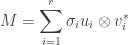This is one version of the singular value decomposition (SVD for short) of $M$ , and it has the benefit of being as close to unique as possible. A more familiar version of SVD is obtained by completing the $v_i$ and $u_i$ to orthonormal bases of $\mathbb{R}^m$ and $\mathbb{R}^n$ (necessarily highly non-unique in general). With respect to these bases, $M$ takes, similar to the warm-up, a block form where the top left block is the diagonal matrix with entries $\sigma_1, \dots \sigma_r$ and the remaining blocks are zero. Hence we can write $M$ as a product

$\displaystyle M = U \Sigma V^T, U \in O(n), V \in O(m)$

where $\Sigma$ has the above block form, $U$ has columns given by $u_1, \dots u_n$ , and $V$ has columns given by $v_1, \dots v_m$ .

So, stepping back a bit: what have we learned about what a linear transformation $T : X \to Y$ between Hilbert spaces looks like? Up to orthogonal change of basis, we’ve learned that they all look like “weighted projections”: we are almost projecting onto the image as in the warmup, except with weights given by the singular values $\sigma_i$ to account for changes in length. The only orthogonal-basis-independent information contained in a linear transformation turns out to be its singular values.

Looking for more analogies between singular value decomposition and the warmup, we might think of the singular values as a quantitative refinement of the rank, since there are $r$ of them where $r$ is the rank, and if some of them are small then $T$ is close (in the operator norm) to a linear transformation having lower rank.

Geometrically, one way to describe the answer provided by singular value decomposition to the question “what does a linear transformation look like” is that the key to understanding $T$ is to understand what it does to the unit sphere of $X$ . The image of the unit sphere is an $r$ -dimensional ellipsoid, and its principal axes have direction given by the left singular vectors $u_i$ and lengths given by the singular values $\sigma_i$ . The right singular vectors $v_i$ map to these.

Properties

Singular value decomposition has lots of useful properties, some of which we’ll prove here. First, note that taking the transpose of a singular value decomposition $M = U \Sigma V^T$ gives another singular value decomposition

$\displaystyle M^T = V \Sigma^T U^T$

showing that $M^T$ has the same singular values as $M$ , but with the left and right singular vectors swapped. This can be proven more conceptually as follows.

Key lemma #2: Write $B(u, v) = \langle u, Mv \rangle = \langle M^T u, v \rangle$ . Then for every $1 \le i \le r$ , the left and right singular vectors $u_i, v_i$ maximize the value of $B(u, v)$ subject to the constraint that $\| u_i \| = \| v_i \| = 1$ for all $i$ , that $u_i$ is orthogonal to $u_j, j \le i-1$ , and that $v_i$ is orthogonal to $v_j, j \le i-1$ . This maximum value is $\sigma_i$ .

Proof. At the maximum value of $B(u, v)$ subject to the constraint that $u$ is orthogonal to $u_j, j \le i-1$ and $v$ is orthogonal to $v_j, j \le i-1$ , it must also be the case that if we fix $v$ then $B(-, v)$ takes its maximum value at $u$ . But for fixed $v$ , $B(u, v) = \langle u, M v \rangle$ uniquely takes its maximum value when $u$ is proportional to $Mv$ (if possible), hence must in fact be equal to $\frac{Mv}{\| M v \|}$ ; moreover, this is always possible thanks to key lemma #1. So we are in fact maximizing

$\displaystyle \left\langle \frac{Mv}{\| M v \|}, M v \right\rangle = \| M v \|$

subject to the above constraints and we already know the solution is given by $v = v_i$ . $\Box$

Left-right symmetry: Let $\sigma_i, u_i, v_i$ be the singular values, left singular vectors, and right singular vectors of $M$ as above. Then $\sigma_i, v_i, u_i$ are the singular values, left singular vectors, and right singular vectors of $M^T$ . In particular, $M^T u_i = \sigma_i v_i$ .

Proof. Apply key lemma #2 to $M^T$ , and note that $B(u, v)$ is the same either way, just with the roles of $u$ and $v$ switched. $\Box$

Singular = eigen: The left singular vectors $u_i$ are the eigenvectors of $M M^T$ corresponding to its nonzero eigenvalues, which are $\sigma_i^2, 1 \le i \le r$ . The right singular vectors $v_i$ are the eigenvectors of $M^T M$ corresponding to its nonzero eigenvalues, which are also $\sigma_i^2, 1 \le i \le r$ .

Proof. We now know that $M v_i = \sigma_i u_i$ and that $M^T u_i = \sigma_i v_i$ , hence

$\displaystyle M^T M v_i = M^T (\sigma_i u_i) = \sigma_i^2 v_i$

and

$\displaystyle M M^T u_i = M (\sigma_i v_i) = \sigma_i^2 u_i$ .

Hence $v_i, u_i$ are orthonormal eigenvectors of $M^T M, M M^T$ respectively. Moreover, these matrices have rank at most (in fact exactly) $r$ , so this exhausts all eigenvectors corresponding to nonzero eigenvalues. $\Box$

This gives an alternative route to understanding singular value decomposition which comes from writing $\| M v \|^2$ as

$\displaystyle \| M v \|^2 = \langle M v, M v \rangle = \langle v, M^T M v \rangle$

and then applying the spectral theorem to $M^T M$ to diagonalize, but I think it’s worth knowing that there’s a route to singular value decomposition which is independent of the spectral theorem.

In addition to the above algebraic characterization of singular values, the singular values also admit the following variational characterization.

Variational characterizations of singular values (Courant, Fischer): We have

$\displaystyle \sigma_k = \max_{V \subseteq \mathbb{R}^m, \dim V = k} \min_{v \in V, \| v \| = 1} \| M v \|$

and

$\displaystyle \sigma_{k+1} = \min_{V \subseteq \mathbb{R}^m, \dim V = m-k} \max_{v \in V, \| v \| = 1} \| M v \|$ .

Proof. For the first characterization, any $k$ -dimensional subspace $V$ intersects $\text{span}(v_k, \dots v_m)$ nontrivially, hence contains a unit vector of the form

$\displaystyle v = \sum_{i=k}^m c_i v_i, \| v \| = \sum_{i=k}^m c_i^2 = 1$ .

We compute that

$\displaystyle M v = \sum_{i=k}^m c_i \sigma_i u_i$

and hence that

$\displaystyle \| M v \|^2 = \sum_{i=k}^m c_i^2 \sigma_i^2 \le \sigma_k^2$ .

We conclude that every $V$ contains $v$ such that $\| M v \| \le \sigma_k$ , hence $\min_{v \in V, \| v \| = 1} \| M v \| \le \sigma_k$ . Equality is obtained when $V = \text{span}(v_1, \dots v_k)$ .

The second characterization is very similar. Any $m-k$ -dimensional subspace $V$ intersects $\text{span}(v_1, \dots v_{k+1})$ nontrivially, hence contains a unit vector of the form

$\displaystyle v = \sum_{i=1}^{k+1} c_i v_i, \| v \| = \sum_{i=1}^{k+1} c_i^2 = 1$ .

We compute that

$\displaystyle M v = \sum_{i=1}^{k+1} c_i \sigma_i u_i$

and hence that

$\displaystyle \| M v \|^2 = \sum_{i=1}^{k+1} c_i^2 \sigma_i^2 \ge \sigma_{k+1}^2$ .

We conclude that every $V$ contains a vector $v$ such that $\| M v \| \ge \sigma_{k+1}$ , hence $\max_{v \in V, \| v \| = 1} \| M v \| \ge \sigma_{k+1}$ . Equality is obtained when $V = \text{span}(v_{k+1}, \dots v_m)$ . $\Box$

The second variational characterization above can be used to prove the following important theorem.

Low rank approximation (Eckart, Young): If $M = U \Sigma V^T$ is the SVD of $M$ , let $M_k = U \Sigma_k V^T$ where $\Sigma_k$ has diagonal entries $\sigma_1, \dots \sigma_k$ and all other entries zero. Then $M_k$ is the closest matrix to $M$ in operator norm with rank at most $k$ ; that is, $M_k$ minimizes $\| M - X \|$ subject to the constraint that $\text{rank}(X) \le k$ . This minimum value is $\sigma_{k+1}$ .

Proof. Suppose $X$ is a matrix of rank at most $k$ . Let $W = \text{ker}(X)$ be the nullspace of $X$ , which by hypothesis has dimension at least $m-k$ . By the second variational characterization above, this means that it contains a vector $w$ such that $\| Mw \| \ge \sigma_{k+1}$ , and since $Xw = 0$ this gives

$\| (M - X) w \| = \| M w \| \ge \sigma_{k+1}$

and hence that $\| M - X \| \ge \sigma_{k+1}$ . Equality is obtained when $X = M_k$ as defined above. $\Box$

The variational characterizations can also be used to prove the following inequality relating the singular values of two matrices and of their sum, which can be thought of as a quantitative refinement of the observation that the rank of a sum $M + N$ of two matrices is at most the sum of their ranks.

Additive perturbation (Weyl): Let $M, N$ be $n \times m$ matrices with singular values $\sigma_i(M), \sigma_i(N)$ . Then

$\displaystyle \sigma_{k+\ell+1}(M+N) \le \sigma_{k+1}(M) + \sigma_{\ell+1}(N)$ .

Proof. We want to bound $\sigma_{k+\ell+1}(M + N)$ in terms of the singular values of $M$ and $N$ . By the second variational characterization, we have

$\displaystyle \sigma_{k+\ell+1}(M + N) = \min_{V \subseteq \mathbb{R}^m, \dim V = m-k-\ell} \max_{v \in V, \| v \| = 1} \| (M + N) v \|$ .

To give an upper bound on a minimum value of a function we just need to give an upper bound on some value that it takes. Let $V_M$ and $V_N$ be the subspaces of $\mathbb{R}^m$ of dimensions $m - k, m - \ell$ respectively which achieve the minimum values of $\max_{v \in V_M, \| v \| = 1} \| M v \|$ and $\max_{v \in V_N, \| v \| = 1} \| N v \|$ respectively, and let $W = V_M \cap V_N$ be their intersection. This intersection has dimension at least $m - k - \ell$ , and by construction

$\displaystyle \max_{v \in W, \| v \| = 1} \| Mv + Nv \| \le \max_{v \in W, \| v \| = 1} \| M v \| + \| N v \| \le \sigma_{k+1}(M) + \sigma_{\ell+1}(N)$ .

Since $W$ has dimension at least $m - k - \ell$ , the above is an upper bound on the value of $\max_{v \in V, \| v \| = 1} \| (M + N) v \|$ for any $(m-k-\ell)$ -dimensional subspace $V \subseteq W$ , from which the conclusion follows. $\Box$

The slightly curious off-by-one indexing in the above inequality can be understood as follows: if $\sigma_{k+1}(M)$ and $\sigma_{\ell+1}(N)$ are both very small, this means that $M$ and $N$ are close to matrices of rank at most $k$ and $\ell$ respectively, and hence $M+N$ is close to a matrix of rank at most $k+\ell$ , hence $\sigma_{k+\ell+1}(M+N)$ also ought to be small.

Setting $\ell = 0$ in the additive perturbation inequality we deduce the following corollary.

Singular values are Lipschitz: The singular values, as functions on matrices, are uniformly Lipschitz with respect to the operator norm with Lipschitz constant $1$ : that is,

$\displaystyle \left| \sigma_k(M) - \sigma_k(N) \right| \le \| M - N \|$ .

Proof. Apply additive perturbation twice with $\ell = 0$ , first to get

$\displaystyle \sigma_k(M) \le \sigma_k(N) + \sigma_1(M-N)$

(remembering that $\sigma_1$ is the operator norm), and second to get

$\displaystyle \sigma_k(N) \le \sigma_k(M) + \sigma_1(N-M)$

(remembering that $\sigma_1(N-M) = \sigma_1(M-N)$ ). $\Box$

This is very much not the case with eigenvalues: a small perturbation of a square matrix can have a large effect on its eigenvalues. This is explained e.g. in in this blog post by Terence Tao, and is related to pseudospectra.

Setting $\sigma_{\ell+1}(N) = 0$ , or equivalently $\text{rank}(N) \le \ell$ , in the additive perturbation inequality, we deduce the following corollary.

Interlacing: Suppose $M, N$ are matrices such that $\text{rank}(M-N) \le \ell$ . Then

$\displaystyle \sigma_{k+\ell}(M) \le \sigma_k(N) \le \sigma_{k-\ell}(M)$ .

Proof. Apply additive perturbation twice, first to get

$\displaystyle \sigma_{k+\ell}(M) \le \sigma_k(N) + \sigma_{\ell+1}(M-N) = \sigma_k(N)$

and second to get

$\displaystyle \sigma_k(N) \le \sigma_{k-\ell}(M) + \sigma_{\ell+1}(N-M) = \sigma_{k-\ell}(M)$ . $\Box$

Interlacing gives us some control over what happens to the singular values under a low-rank perturbation (as opposed to a low-norm perturbation; a low-rank perturbation may have arbitrarily high norm, and vice versa). For example, we learn that if all of the singular values are clumped together, then a rank- $\ell$ perturbation will keep most of the singular values clumped together, except possibly for either the $\ell$ largest or $\ell$ smallest singular values. We can’t expect any control over these, since in the worst case a rank- $\ell$ perturbation can make the $\ell$ largest singular values arbitrarily large, or make the $\ell$ smallest singular values arbitrarily small.

A particular special case of a low-rank perturbation is deleting a small number of rows or columns (note that a row or column which is entirely zero does not affect the singular values, so deleting a row or column is equivalent to setting all of its entries to zero), in which case the upper bound above can be tightened.

Cauchy interlacing: Suppose $M$ is a matrix and $N$ is obtained from $M$ by deleting at most $\ell$ rows. Then

$\displaystyle \sigma_k(M) \ge \sigma_k(N) \ge \sigma_{k+\ell}(M)$ .

Proof. The lower bound follows from interlacing. The upper bound follows from the observation that we have $\| N v \| \le \| M v \|$ for all $v$ , then applying either variational characterization of the singular values. $\Box$

Cauchy interlacing also applies to deleting columns, or combinations of rows and columns, because the singular values are unchanged by transposition. In particular, we learn that if $N$ is obtained from $M$ by deleting either a single row or a single column, then the singular values of $N$ interlace with the singular values of $M$ , hence the name.

In particular, if all of the singular values of $M$ are clumped together then so are those of $N$ , with no exceptions. Taking the contrapositive, if the singular values of $N$ are spread out, then the singular values of $M$ must be as well.

Three special cases

Three special cases of the general singular value decomposition $M = U \Sigma V^T$ are worth pointing out.

First, if $M$ has orthogonal columns, or equivalently if $M^T M$ is diagonal, then the singular values $\sigma_i$ are the lengths of its columns, we can take the right singular vectors to be the standard basis vectors $v_i = e_i$ , and we can take the left singular vectors to be the unit rescalings of its columns. This means that we can take $V = I$ to be the identity matrix, and in general suggests that $\| I - V \|$ is a measure of the extent to which the columns of $M$ fail to be orthogonal (with the caveat that $V$ is not unique and so in general we would want to look at the $V$ closest to $I$ ).

Second, if $M$ has orthogonal rows, or equivalently if $M M^T$ is diagonal, then the singular values $\sigma_i$ are the lengths of its rows, we can take the left singular vectors to be the standard basis vectors $u_i = e_i$ , and we can take the right singular vectors to be the unit rescalings of its rows. This means that we can take $U = I$ to be the identity matrix, and in general suggests that $\| I - U \|$ is a measure of the extent to which the rows of $M$ fail to be orthogonal (with the same caveat as above).

Finally, if $M$ is square and an orthogonal matrix, so that $M^T M = M M^T = I$ , then the singular values $\sigma_i$ are all equal to $1$ , and an arbitrary choice of either the left or the right singular vectors uniquely determines the other. This means that we can take $\Sigma = I$ to be the identity matrix, and in general suggests that $\| I - \Sigma \|$ is a measure of the extent to which $M$ fails to be orthogonal. In fact it is possible to show that the closest orthogonal matrix to $M = U \Sigma V^T$ is given by $U V^T$ , or in other words by replacing all of the singular values of $M$ with $1$ , so

$\displaystyle \| I - \Sigma \| = \max_i |1 - \sigma_i|$

is precisely the distance from $M$ to the nearest orthogonal matrix. This fact can be used to solve the orthogonal Procrustes problem.

In general, we should expect that the SVD of a matrix $M$ is relevant to answering any question about $M$ whose answer is invariant under left and right multiplication by orthogonal matrices. This includes, for example, the question of low-rank approximations to $M$ with respect to operator norm we answered above, since both rank and operator norm are invariant.

http://qchu.wordpress.com/?p=27043

Extensions

Higher linear algebra

Qiaochu Yuan May 31, 2016

Let be a commutative ring. A popular thing to do on this blog is to think about the Morita 2-category of algebras, bimodules, and bimodule homomorphisms over , but it might be unclear exactly what we’re doing when we do this. What are we studying when we study the Morita 2-category? The answer is that […]

Show full content

Let $k$ be a commutative ring. A popular thing to do on this blog is to think about the Morita 2-category $\text{Mor}(k)$ of algebras, bimodules, and bimodule homomorphisms over $k$ , but it might be unclear exactly what we’re doing when we do this. What are we studying when we study the Morita 2-category?

The answer is that we can think of the Morita 2-category as a 2-category of module categories over the symmetric monoidal category $\text{Mod}(k)$ of $k$ -modules, equipped with the usual tensor product $\otimes_k$ over $k$ . By the Eilenberg-Watts theorem, the Morita 2-category is equivalently the 2-category whose

objects are the categories $\text{Mod}(A)$ , where $A$ is a $k$ -algebra,
morphisms are cocontinuous $k$ -linear functors $\text{Mod}(A) \to \text{Mod}(B)$ , and
2-morphisms are natural transformations.

An equivalent way to describe the morphisms is that they are “ $\text{Mod}(k)$ -linear” in that they respect the natural action of $\text{Mod}(k)$ on $\text{Mod}(A)$ given by

$\displaystyle \text{Mod}(k) \times \text{Mod}(A) \ni (V, M) \mapsto V \otimes_k M \in \text{Mod}(A)$ .

This action comes from taking the adjoint of the enrichment of $\text{Mod}(A)$ over $\text{Mod}(k)$ , which gives a tensoring of $\text{Mod}(A)$ over $\text{Mod}(k)$ . Since the two are related by an adjunction in this way, a functor respects one iff it respects the other.

So Morita theory can be thought of as a categorified version of module theory, where we study modules over $\text{Mod}(k)$ instead of over $k$ . In the simplest cases, we can think of Morita theory as a categorified version of linear algebra, and in this post we’ll flesh out this analogy further.

Technical preliminaries

Let $(V, \otimes)$ be a symmetric monoidal category (which in this post will be $\text{Mod}(k)$ , for $k$ a commutative ring), and consider categories enriched over $V$ , or $V$ -categories for short. If $C$ and $D$ are two $V$ -categories, their naive tensor product $C \otimes D$ is the $V$ -category whose objects are pairs $(c, d)$ of objects in $C$ and objects in $D$ , and whose homs are given by the tensor products

$\text{Hom}_{C \otimes D}((c_1, d_1), (c_2, d_2)) \cong \text{Hom}_C(c_1, c_2) \otimes \text{Hom}_D(d_1, d_2)$

of the homs in $C$ and $D$ , with the obvious composition (which requires the ability to switch tensor factors to define). When $C$ and $D$ have one object and $V = \text{Mod}(k)$ , this reduces to the usual tensor product of $k$ -algebras.

Thinking of $V$ -categories as many-object generalizations of $V$ -algebras (one might call them “ $V$ -algebroids,” but I won’t), it’s natural to define notions of modules over them. We’ll say that a left module over $C$ is a $V$ -functor ( $V$ -enriched functor) $C \to V$ , while a right module over $C$ is a $V$ -functor $C^{op} \to V$ . If $C, D$ are two $V$ -categories, a $(C, D)$ -bimodule is a $V$ -functor $D^{op} \otimes C \to V$ .

All of this terminology has its usual meaning when $C$ and $D$ have one object (so correspond to algebras) and $V = \text{Mod}(k)$ .

The basic analogy

The basic analogy, one piece of structure at a time, goes like this.

Sets are analogous to categories.
Abelian groups are analogous to cocomplete categories. (There are several other things we could have said here, but this is the one that’s relevant to thinking about Morita theory. The idea is that taking colimits categorifies addition.)
Rings are analogous to monoidal cocomplete categories (this includes the condition that the monoidal structure distributes over colimits).
Commutative rings are analogous to symmetric monoidal cocomplete categories.
Modules over commutative rings are analogous to cocomplete module categories over symmetric monoidal cocomplete categories.

We won’t get into the generalities of thinking about symmetric monoidal categories or modules over them because, in this post, the only symmetric monoidal categories we care about are those of the form $\text{Mod}(k)$ for a commutative ring $k$ , and the only module categories over them we care about are the ones that are “free on a category of generators” in the sense that they are categories of $k$ -linear presheaves / right modules

$\displaystyle \text{Mod}(C) \cong [C^{op}, \text{Mod}(k)]$

on essentially small $k$ -linear categories $C$ (thinking of taking presheaves as the free cocompletion). By the universal property of the free cocompletion, cocontinuous $k$ -linear functors $\text{Mod}(C) \to \text{Mod}(D)$ correspond to $k$ -linear functors $C \to \text{Mod}(D)$ , or equivalently (by an adjunction) to $(C, D)$ -bimodules; this generalizes, and in particular proves, the Eilenberg-Watts theorem. Composition is given by tensor product of bimodules, which is computed using coends.

In the special case that the categories $C, D$ involved have one object, they correspond to $k$ -algebras, and the words “module,” “bimodule,” and “tensor product” all have their usual meaning. More generally, if $C$ has finitely many isomorphism classes of objects, then we can replace it with the endomorphism ring of the direct sum of one object from each isomorphism class (because $C$ is Morita equivalent to the one-object $k$ -linear category with this endomorphism ring), so we get a genuinely bigger Morita 2-category if we allow $C$ to have infinitely many objects.

From now on we’ll work in this bigger Morita 2-category, which is now the 2-category deserving the name $\text{Mor}(k)$ . It has

objects essentially small $k$ -linear categories $C$ ,
morphisms $(C, D)$ -bimodules over $k$ , and
2-morphisms homomorphisms of bimodules.

Equivalently, it has

objects the cocomplete $k$ -linear categories $\text{Mod}(C)$ (where $C$ is as above),
morphisms cocontinuous $k$ -linear functors $\text{Mod}(C) \to \text{Mod}(D)$ , and
2-morphisms natural transformations.

From now on, when we say that a $k$ -linear category $C$ “is” a $k$ -algebra, possibly with some further properties, what we mean is that it’s equivalent to a category with one object and endomorphism ring a $k$ -algebra, possibly with some further properties.

In what ways do the objects of the Morita 2-category behave like modules?

Proposition: The Morita 2-category has biproducts.

In other words, the product $\text{Mod}(A) \times \text{Mod}(B)$ is also the coproduct. This is because on the one hand a functor (cocontinuous and $k$ -linear) into $\text{Mod}(A) \times \text{Mod}(B)$ is precisely a pair of functors into $\text{Mod}(A)$ and $\text{Mod}(B)$ , and on the other hand

$\displaystyle \text{Mod}(A) \times \text{Mod}(B) \cong \text{Mod}(A \sqcup B).$

If $A$ and $B$ are algebras rather than categories it would be tempting to write $A \times B$ rather than $A \sqcup B$ , but in the case of algebras these are Morita equivalent as $k$ -linear categories. Actually, the above argument, with disjoint unions of $k$ -linear categories, applies just as well to infinitely many $k$ -linear categories: this means that the bigger Morita 2-category has infinite biproducts. Note that this has nothing to do with $\text{Mod}(k)$ itself having biproducts: the same is true for the bigger Morita 2-category over $\text{Set}$ .

Proposition: There is a tensor-hom adjunction

$\displaystyle [\text{Mod}(A) \otimes \text{Mod}(B), \text{Mod}(C)] \cong [\text{Mod}(A), [\text{Mod}(B), \text{Mod}(C)]]$ .

Here the internal hom $[-, -]$ is the category of cocontinuous $k$ -linear functors, which (as we’ve seen above, since it’s a category of bimodules) is itself a cocomplete $k$ -linear category, and the tensor product $\otimes$ is

$\displaystyle \text{Mod}(A) \otimes \text{Mod}(B) \cong \text{Mod}(A \otimes_k B)$

(this is a computation, not a definition: the definition is a universal property in terms of functors out of $\text{Mod}(A) \times \text{Mod}(B)$ which are cocontinuous and $k$ -linear in each variable). Here $A \otimes_k B$ is the “naive” tensor product over $k$ .

Both sides of the equivalence above are equivalent to $\text{Mod}(A^{op} \otimes_k B^{op} \otimes_k C)$ , which might look familiar as a categorification of a corresponding statement about finite-dimensional vector spaces. This reflects the fact that $\text{Mod}(C)$ is always dualizable with respect to the above tensor product, with dual $\text{Mod}(C^{op})$ .

With respect to this tensor product, $\text{Mod}(k)$ is the unit object. It should be thought of as the “tensor product over $\text{Mod}(k)$ ,” exactly analogous to the tensor product on modules over a commutative ring.

Aside: big categories vs. little categories

The biggest secret about category theory that I don’t think is in common circulation is that there are approximately two kinds of categories, and they should be thought of very differently (because the relevant notion of morphism between them is very different):

Big categories are “categories of mathematical objects.” Typical examples are categories of modules and sheaves. They tend to be cocomplete, and people like to consider cocontinuous functors (really, left adjoints) between them.
Little categories are “categories as mathematical objects.” Typical examples include categories with one object, or finitely many objects. They tend to be Cauchy complete at best, and people like to consider arbitrary functors, or more generally bimodules, between them.

The Morita 2-categories we discussed above have both little descriptions and big descriptions (via $k$ -linear categories and modules over these respectively), and both are important. We can pass from little to big by taking modules / presheaves, and we can pass from big to little by taking tiny objects. (This can at best recover the Cauchy completion of the original little $k$ -linear category, but this is fine since we’re only hoping to doing things up to Morita equivalence anyway.)

I think one thing that confuses people when they first start to learn category theory is that the first examples of categories (e.g. groups, rings, modules) tend to be big, even though little categories figure prominently in the theory (e.g. as shapes for diagrams to take limits or colimits over, and/or as things to take presheaves or sheaves on) and feel very different. It’s little categories that can reasonably be thought of as algebraic objects generalizing more familiar objects like monoids and posets (or, in our enriched setting, $k$ -algebras), whereas big categories, I think, genuinely require a new set of intuitions.

On the other hand, the ability to pass between big and little categories is also important. Eilenberg-Watts, as we have seen, gives one version of this: another version is Gabriel-Ulmer duality.

The big vs. little nomenclature suggests, but is not equivalent to, the rigorous distinction between large and small categories, and is related to the distinction between big and little toposes (or, depending on your preferences, between gros and petit topoi) in sheaf theory. The basic point of this distinction is that there are two somewhat different sorts of things people mean by sheaf: on the one hand one might mean a functor on a little category like the category of open subsets of a topological space, and on the other hand one might mean a functor on a big category like the category of commutative rings. It would be nice if people emphasized this distinction more.

Bases, coordinates, and matrices

In terms of higher linear algebra, big categories of modules are “higher vector spaces,” while the little categories that can be used to present the big categories as categories of modules are “bases” for them. As we learned previously, a cocomplete abelian category has a “basis” in this sense iff it has a family of tiny (compact projective) generators, for various notions of generator.

Given a “basis” $C$ for a “higher vector space” $\text{Mod}(C)$ (really, a higher module), any object is described by a module / presheaf $F : C^{op} \to \text{Mod}(k)$ ; the components of this presheaf can be thought of as the “coordinates” of $F$ in the “basis” $C$ . In the same way that a vector is a sum over elements of a basis weighted by its coordinates in that basis, a presheaf is a weighted colimit / coend / functor tensor product

$\displaystyle F(-) \cong \int^{c \in C} F(c) \otimes_k \text{Hom}(-, c)$

weighted by its “coordinates” $F(c)$ of the “basis” of representable presheaves. This is an enriched version of the familiar statement that a presheaf of sets over a category is canonically a colimit of representable presheaves. It is sometimes called the co-Yoneda lemma.

Similarly, the statement that cocontinuous $k$ -linear functors $\text{Mod}(C) \to \text{Mod}(D)$ are equivalent to functors $C \otimes_k D^{op} \to \text{Mod}(k)$ can be interpreted as saying that such functors can be written as “matrices” indexed by $C$ and $D$ . Composition, as well as evaluation, are given by the familiar formulas if we consistently reinterpret the relevant products as tensor products and the relevant sums as coends.

Suppose in particular that $C = D$ . Then we get that endomorphisms of $\text{Mod}(C)$ correspond to $(C, C)$ -bimodules, or equivalently to functors $F : C^{op} \otimes_k C \to \text{Mod}(k)$ . These are precisely the sorts of things we can take coends of, getting an object

$\displaystyle \text{Tr}(F) = \int^{c \in C} F(c, c) \in \text{Mod}(k)$

which deserves to be called the trace of the endomorphism $F$ . This is a generalization of (zeroth) Hochschild homology with coefficients in a bimodule, which it reduces to when $C$ is an algebra. (There is also a second trace generalizing Hochschild cohomology and computed using ends.)

The identity functor turns out to be represented by $\text{Hom}(-, -)$ , so taking its trace we get the Hochschild homology or trace of $C$ (or, depending on your point of view, of $\text{Mod}(C)$ ) itself:

$\displaystyle \text{Tr}(C) = \int^{c \in C} \text{Hom}(c, c) \in \text{Mod}(k)$ .

More explicitly, this coend is the result of coequalizing the left and right actions of $C$ on $\text{Hom}(-, -)$ (by postcomposition and precomposition respectively), so can be written as

$\displaystyle \text{Tr}(C) = \text{coeq} \left( \coprod_{c, d \in C} \text{Hom}(c, d) \otimes \text{Hom}(d, c) \rightrightarrows \coprod_{c \in C} \text{Hom}(c, c) \right)$

where the two arrows send a pair of morphisms $f : c \to d$ and $g : d \to c$ to the two composites $fg : d \to d$ and $gf : c \to c$ . In other words, $\text{Tr}(C)$ is the quotient of the direct sum of the endomorphism rings of every object in $C$ by the subspace of “commutators” of the form $fg - gf$ , where $f, g$ need not themselves be endomorphisms.

By construction, this means that $\text{Tr}(C)$ is the recipient of a “universal trace” map: any endomorphism $h : c \to c$ in $C$ has an image $\text{tr}(h) \in \text{Tr}(C)$ satisfying

$\displaystyle \text{tr}(fg) = \text{tr}(gf)$

for all $f, g$ as above, and $\text{Tr}(C)$ is universal with respect to this property.

Example. Suppose $C$ has one object, so corresponds to an algebra $A$ . Then $\text{tr}(C)$ is just the quotient $A/[A, A]$ of $A$ by the subspace of commutators, hence is the ordinary zeroth Hochschild cohomology $HH^0(A)$ of $A$ (with coefficients in itself).

The above construction of the trace implies that it is Morita invariant, and $A$ is Morita equivalent to the $k$ -linear category of finitely generated projective (right) $A$ -modules (which is its Cauchy completion). It follows that the trace of this category is also $A/[A, A]$ , and this means that for any finitely generated projective $A$ -module $M$ and any endomorphism $f : M \to M$ there is a trace

$\displaystyle \text{tr}(f) \in A/[A, A]$ .

This trace is called the Hattori-Stallings trace. For free modules it is computed by taking the image of the sum of the diagonal elements of $f$ in $A/[A, A]$ . It is a shadow of various more general and more interesting maps from versions of K-theory to versions of Hochschild homology, including a version of the Chern character and the Dennis trace.

In particular, if $A$ is commutative, we recover the usual notion of trace of an endomorphism of a finitely generated projective $A$ -module without using a monoidal structure (previously we recovered this notion using dualizability with respect to the usual tensor product of $A$ -modules).

The simplest interesting case of the above discussion occurs when $k$ is a field and the algebras we consider are finite direct sums of matrix algebras $M_n(k)$ ; equivalently, the $\text{Vect}(k)$ -module categories we consider are finite direct sums of copies of $\text{Vect}(k)$ . These are known as Kapranov-Voevodsky 2-vector spaces. Morphisms from $\text{Vect}(k)^n$ to $\text{Vect}(k)^m$ correspond to $m \times n$ matrices of vector spaces, just as for free modules, and the trace of an endomorphism $\text{Vect}(k)^n \to \text{Vect}(k)^n$ is the direct sum of its diagonal vector spaces.

Higher representation theory

One reason you might want a higher version of linear algebra is to study “higher representation theory,” where groups (or higher versions of groups, such as 2-groups) act on higher vector spaces. Previously we saw such actions occur naturally in Galois descent: namely, if $k \to L$ is a Galois extension with Galois group $G$ , then $G$ naturally acts on the category $\text{Mod}(L)$ of $L$ -vector spaces, and we used this action to describe Galois descent for vector spaces.

More generally, if $G$ is a group acting on a scheme $X$ (or some more or less general object, depending on taste), then $G$ naturally acts on the category $QC(X)$ of quasicoherent sheaves on $X$ . If $X$ is an $S$ -scheme for some base $S$ , this is naturally a module category over $QC(S)$ , and if $G$ acts on $X$ by $S$ -scheme automorphisms, the induced action on $QC(X)$ is $QC(S)$ -linear. One reason you might want to understand higher representation theory is to understand these sorts of actions. In particular, a natural question is what the homotopy fixed points of this action are, and the answer is that

$\displaystyle QC(X)^G \cong QC(X/G)$ ;

that is, the homotopy fixed point category (which here is typically called “ $G$ -equivariant quasicoherent sheaves on $X$ “) is the category of quasicoherent sheaves on the quotient $X/G$ regarded as a stack. (It certainly does not suffice to take the ordinary quotient of schemes: for example, if $X = \text{Spec } k$ is a point, then $X/G$ is $BG$ , and $QC(\text{Spec } k)^G \cong QC(BG)$ is the category of $k$ -linear representations of $G$ .)

If the stacky quotient $X/G$ happens to be an ordinary scheme (so $X \to X/G$ is a $G$ -torsor in schemes), this is a generalization of Galois descent, to which it reduces in the case when $k \to L$ is a finite extension, $X = \text{Spec } L$ , and $G$ is the Galois group.

http://qchu.wordpress.com/?p=24595

Extensions

What’s a fire, and why does it – what’s the word – burn?

Qiaochu Yuan May 26, 2016

I was staring at a bonfire on a beach the other day and realized that I didn’t understand anything about fire and how it works. (For example: what determines its color?) So I looked up some stuff, and here’s what I learned. Fire Fire is a sustained chain reaction involving combustion, which is an exothermic reaction in […]

Show full content

Fire

Fire is a sustained chain reaction involving combustion, which is an exothermic reaction in which an oxidant, typically oxygen, oxidizes a fuel, typically a hydrocarbon, to produce products such as carbon dioxide, water, and heat and light. A typical example is the combustion of methane, which looks like

$\displaystyle \text{CH}_4 + 2 \text{ O}_2 \to \text{CO}_2 + 2 \text{ H}_2 \text{O}$ .

The heat produced by combustion can be used to fuel more combustion, and when that happens enough that no additional energy needs to be added to sustain combustion, you’ve got a fire. To stop a fire, you can remove the fuel (e.g. turning off a gas stove), remove the oxidant (e.g. smothering a fire using a fire blanket), remove the heat (e.g. spraying a fire with water), or remove the combustion reaction itself (e.g. with halon).

Combustion is in some sense the opposite of photosynthesis, an endothermic reaction which takes in light, water, and carbon dioxide and produces hydrocarbons.

It’s tempting to assume that when burning wood, the hydrocarbons that are being combusted are e.g. the cellulose in the wood. It seems, however, that something more complicated happens. When wood is exposed to heat, it undergoes pyrolysis (which, unlike combustion, doesn’t involve oxygen), which converts it to more flammable compounds, such as various gases, and these are what combust in wood fires.

When a wood fire burns for long enough it will lose its flame but continue to smolder, and in particular the wood will continue to glow. Smoldering involves incomplete combustion, which, unlike complete combustion, produces carbon monoxide.

Flames

Flames are the visible parts of a fire. As fires burn, they produce soot (which can refer to some of the products of incomplete combustion or some of the products of pyrolysis), which heats up, producing thermal radiation. This is one of the mechanisms responsible for giving fire its color. It is also how fires warm up their surroundings.

Thermal radiation is produced by the motion of charged particles: anything at positive temperature consists of charged particles moving around, so emits thermal radiation. A more common but arguably less accurate term is black body radiation; this properly refers to the thermal radiation emitted by an object which absorbs all incoming radiation. It’s common to approximate thermal radiation by black body radiation, or by black body radiation times a constant, because it has the useful property that it depends only on the temperature of the black body. Black body radiation happens at all frequencies, with more radiation at higher frequencies at higher temperatures; in particular, the peak frequency is directly proportional to temperature by Wien’s displacement law.

Everyday objects are constantly producing thermal radiation, but most of it is infrared – its wavelength is longer than that of visible light, and so is invisible without special cameras. Fires are hot enough to produce visible light, although they are still producing a lot of infrared light.

Another mechanism giving fire its color is the emission spectra of whatever’s being burned. Unlike black body radiation, emission spectra occur at discrete frequencies; this is caused by electrons producing photons of a particular frequency after transitioning from a higher-energy state to a lower-energy state. These frequencies can be used to detect elements present in a sample in flame tests, and a similar idea (using absorption spectra) is used to determine the composition of the sun and various stars. Emission spectra are also responsible for the color of fireworks and of colored fire.

The characteristic shape of a flame on Earth depends on gravity. As a fire heats up the surrounding air, natural convection occurs: the hot air (which contains, among other things, hot soot) rises, while cool air (which contains oxygen) falls, sustaining the fire and giving flames their characteristic shape. In low gravity, such as on a space station, this no longer occurs; instead, fires are only fed by the diffusion of oxygen, and so burn more slowly and with a spherical shape (since now combustion is only happening at the interface of the fire with the parts of the air containing oxygen; inside the sphere there is presumably no more oxygen to burn):

candles-reg-microgravz

Black body radiation

Black body radiation is described by Planck’s law, which is fundamentally quantum mechanical in nature, and which was historically one of the first applications of any form of quantum mechanics. It can be deduced from (quantum) statistical mechanics as follows.

What we’ll actually compute is the distribution of frequencies in a (quantum) gas of photons at some temperature $T$ ; the claim that this matches the distribution of frequencies of photons emitted by a black body at the same temperature comes from a physical argument related to Kirchhoff’s law of thermal radiation. The idea is that the black body can be put into thermal equilibrium with the gas of photons (since they have the same temperature). The gas of photons is getting absorbed by the black body, which is also emitting photons, so in order for them to stay in equilibrium, it must be the case that at every frequency the black body is emitting radiation at the same rate as it’s absorbing it, which is determined by the distribution of frequencies in the gas. (Or something like that. I Am Not A Physicist, so if your local physicist says different then believe them instead.)

In statistical mechanics, the probability of finding a system in microstate $s$ given that it’s in thermal equilibrium at temperature $T$ is proportional to

$\displaystyle e^{- \beta E_s}$

where $E_s$ is the energy of state $s$ and $\beta = \frac{1}{k_B T}$ is thermodynamic beta (so $T$ is temperature and $k_B$ is Boltzmann’s constant); this is the Boltzmann distribution. For one possible justification of this, see this blog post by Terence Tao. This means that the probability is

$\displaystyle p_s = \frac{1}{Z(\beta)} e^{-\beta E_s}$

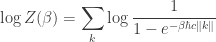
where $Z(\beta)$ is the normalizing constant

$\displaystyle Z(\beta) = \sum_s e^{-\beta E_s}$

called the partition function. Note that these probabilities don’t change if $E_s$ is modified by an additive constant (which multiplies the partition function by a constant); only differences in energy between states matter.

It’s a standard observation that the partition function, up to multiplicative scale, contains the same information as the Boltzmann distribution, so anything that can be computed from the Boltzmann distribution can be computed from the partition function. For example, the moments of the energy are given by

$\displaystyle \langle E^k \rangle = \frac{1}{Z} \sum_s E_s^k e^{-\beta E_s} = \frac{(-1)^k}{Z} \frac{\partial^k}{\partial \beta^k} Z$

and, up to solving the moment problem, this characterizes the Boltzmann distribution. In particular, the average energy is

$\displaystyle \langle E \rangle = - \frac{\partial}{\partial \beta} \log Z$ .

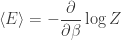The Boltzmann distribution can be used as a definition of temperature. It correctly suggests that in some sense $\beta$ is the more fundamental quantity because it might be zero (meaning every microstate is equally likely; this corresponds to “infinite temperature”) or negative (meaning higher-energy microstates are more likely; this corresponds to “negative temperature,” which it is possible to transition to after “infinite temperature,” and which in particular is hotter than every positive temperature).

To describe the state of a gas of photons we’ll need to know something about the quantum behavior of photons. In the standard quantization of the electromagnetic field, the electromagnetic field can be treated as a collection of quantum harmonic oscillators each oscillating at various (angular) frequencies $\omega$ . The energy eigenstates of a quantum harmonic oscillator are labeled by a nonnegative integer $n \in \mathbb{Z}_{\ge 0}$ , which can be interpreted as the number of photons of frequency $\omega$ . The energies of these eigenstates are (up to an additive constant, which doesn’t matter for this calculation and so which we will ignore)

$\displaystyle E_n = n \hbar \omega$

where $\hbar$ is the reduced Planck constant. The fact that we only need to keep track of the number of photons rather than distinguishing them reflects the fact that photons are bosons. Accordingly, for fixed $\omega$ , the partition function is

$\displaystyle Z_{\omega}(\beta) = \sum_{n=0}^{\infty} e^{-n \beta \hbar \omega} = \frac{1}{1 - e^{-\beta \hbar \omega}}$ .

Digression: the (wrong) classical answer

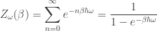The assumption that $n$ , or equivalently the energy $E_n = n \hbar \omega$ , is required to be an integer here is the Planck postulate, and historically it was perhaps the first appearance of a quantization (in the sense of quantum mechanics) in physics. Without this assumption (so using classical harmonic oscillators), the sum above becomes an integral (where $n$ is now proportional to the square of the amplitude), and we get a “classical” partition function

$\displaystyle Z_{\omega}^{cl}(\beta) = \int_0^{\infty} e^{-n \beta \hbar \omega} \, dn = \frac{1}{\beta \hbar \omega}$ .

(It’s unclear what measure we should be integrating against here, but but this calculation appears to reproduce the usual classical answer, so I’ll stick with it.)

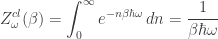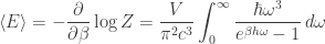
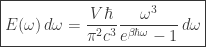
These two partition functions give very different predictions, although the quantum one approaches the classical one as $\beta \hbar \omega \to 0$ . In particular, the average energy of all photons of frequency $\omega$ , computed using the quantum partition function, is

$\displaystyle \langle E \rangle_{\omega} = - \frac{d}{d \beta} \log \frac{1}{1 - e^{-\beta \hbar \omega}} = \frac{\hbar \omega}{e^{\beta \hbar \omega} - 1}$

whereas the average energy computed using the classical partition function is

$\displaystyle \langle E \rangle_{\omega}^{cl} = - \frac{d}{d \beta} \log \frac{1}{\beta \hbar \omega} = \frac{1}{\beta} = k_B T$ .

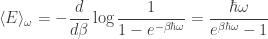
The quantum answer approaches the classical answer as $\hbar \omega \to 0$ (so for small frequencies), and the classical answer is consistent with the equipartition theorem in classical statistical mechanics, but it is also grossly inconsistent with experiment and experience. It predicts that the average energy of the radiation emitted by a black body at a frequency $\omega$ is a constant independent of $\omega$ , and since radiation can occur at arbitrarily high frequencies, the conclusion is that a black body is emitting an infinite amount of energy, at every possible frequency, which is of course badly wrong. This is (most of) the ultraviolet catastrophe.

The quantum partition function instead predicts that at low frequencies (relative to the temperature) the classical answer is approximately correct, but that at high frequencies the average energy becomes exponentially damped, with more damping at lower temperatures. This is because at high frequencies and low temperatures a quantum harmonic oscillator spends most of its time in its ground state, and cannot easily transition to its next lowest state, which is exponentially less likely. Physicists say that most of this “degree of freedom” (the freedom of an oscillator to oscillate at a particular frequency) gets “frozen out.” The same phenomenon is responsible for classical but incorrect computations of specific heat, e.g. for diatomic gases such as oxygen.

The density of states and Planck’s law

Now that we know what’s going on at a fixed frequency $\omega$ , it remains to sum over all possible frequencies. This part of the computation is essentially classical and no quantum corrections to it need to be made.

We’ll make a standard simplifying assumption that our gas of photons is trapped in a box with side length $L$ subject to periodic boundary conditions (so really, the flat torus $T = \mathbb{R}^3/L \mathbb{Z}^3$ ); the choice of boundary conditions, as well as the shape of the box, will turn out not to matter in the end. Possible frequencies are then classified by standing wave solutions to the electromagnetic wave equation in the box with these boundary conditions, which in turn correspond (up to multiplication by $c$ ) to eigenvalues of the Laplacian $\Delta$ . More explicitly, if $\Delta v = \lambda v$ , where $v(x)$ is a smooth function $T \to \mathbb{R}$ , then the corresponding standing wave solution of the electromagnetic wave equation is

$\displaystyle v(t, x) = e^{c \sqrt{\lambda} t} v(x)$

and hence (keeping in mind that $\lambda$ is typically negative, so $\sqrt{\lambda}$ is typically purely imaginary) the corresponding frequency is

$\displaystyle \omega = c \sqrt{-\lambda}$ .

This frequency occurs $\dim V_{\lambda}$ times where $V_{\lambda}$ is the $\lambda$ -eigenspace of the Laplacian.

The reason for the simplifying assumptions above are that for a box with periodic boundary conditions (again, mathematically a flat torus) it is very easy to explicitly write down all of the eigenfunctions of the Laplacian: working over the complex numbers for simplicity, they are given by

$\displaystyle v_k(x) = e^{i k \cdot x}$

where $k = \left( k_1, k_2, k_3 \right) \in \frac{2 \pi}{L} \mathbb{Z}^3$ is the wave vector. (Somewhat more generally, on the flat torus $\mathbb{R}^n/\Gamma$ where $\Gamma$ is a lattice, wave numbers take values in the dual lattice of $\Gamma$ , possibly up to scaling by $2 \pi$ depending on conventions). The corresponding eigenvalue of the Laplacian is

$\displaystyle \lambda_k = - \| k \|^2 = - k_1^2 - k_2^2 - k_3^2$

from which it follows that the multiplicity of a given eigenvalue $- \frac{4 \pi^2}{L^2} n$ is the number of ways to write $n$ as a sum of three squares. The corresponding frequency is

$\displaystyle \omega_k = c \| k \|$

and so the corresponding energy (of a single photon with that frequency) is

$\displaystyle E_k = \hbar \omega_k = \hbar c \| k \|$ .

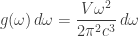
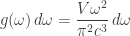
At this point we’ll approximate the probability distribution over possible frequencies $\omega_k$ , which is strictly speaking discrete, as a continuous probability distribution, and compute the corresponding density of states $g(\omega)$ ; the idea is that $g(\omega) \, d \omega$ should correspond to the number of states available with frequencies between $\omega$ and $\omega + d \omega$ . Then we’ll do an integral over the density of states to get the final partition function.

Why is this approximation reasonable (unlike the case of the partition function for a single harmonic oscillator, where it wasn’t)? The full partition function can be described as follows. For each wavenumber $k \in \frac{2\pi}{L} \mathbb{Z}^3$ , there is an occupancy number $n_k \in \mathbb{Z}_{\ge 0}$ describing the number of photons with that wavenumber; the total number $n = \sum n_k$ of photons is finite. Each such photon contributes $\hbar \omega_k = \hbar c \| k \|$ to the energy, from which it follows that the partition function factors as a product

$\displaystyle Z(\beta) = \prod_k Z_{\omega_k}(\beta) = \prod_k \frac{1}{1 - e^{- \beta \hbar c \| k \|}}$

over all wave numbers $k$ , hence that its logarithm factors as a sum

$\displaystyle \log Z(\beta) = \sum_k \log \frac{1}{1 - e^{-\beta \hbar c \| k \|}}$ .

and it is this sum that we want to approximate by an integral. It turns out that for reasonable temperatures and reasonably large boxes, the integrand varies very slowly as $k$ varies, so the approximation by an integral is very close. The approximation stops being reasonably only at very low temperatures, where as above quantum harmonic oscillators mostly end up in their ground states and we get Bose-Einstein condensates.

The density of states can be computed as follows. We can think of wave vectors as evenly spaced lattice points living in some “phase space,” from which it follows that the number of wave vectors in some region of phase space is proportional to its volume, at least for regions which are large compared to the lattice spacing $\frac{2 \pi}{L}$ . In fact, the number of wave vectors in a region of phase space is exactly $\frac{V}{8 \pi^3}$ times the volume, where $V = L^3$ is the volume of our box / torus.

It remains to compute the volume of the region of phase space given by all wave vectors $k$ with frequencies $\omega_k = c \| k \|$ between $\omega$ and $\omega + d \omega$ . This region is a spherical shell with thickness $\frac{d \omega}{c}$ and radius $\frac{\omega}{c}$ , and hence its volume is

$\displaystyle \frac{4 \pi \omega^2}{c^3} \, d \omega$

from which we get that the density of states for a single photon is

$\displaystyle g(\omega) \, d \omega = \frac{V \omega^2}{2 \pi^2 c^3} \, d \omega$ .

Actually this formula is off by a factor of two: we forgot to take photon polarization into account (equivalently, photon spin), which doubles the number of states with a given wave number, giving the corrected density

$\displaystyle g(\omega) \, d \omega = \frac{V \omega^2}{\pi^2 c^3} \, d \omega$ .

The fact that the density of states is linear in the volume $V$ is not specific to the flat torus; it’s a general feature of eigenvalues of the Laplacian by Weyl’s law. This gives that the logarithm of the partition function is

$\displaystyle \log Z = \frac{V}{\pi^2 c^3} \int_0^{\infty} \omega^2 \log \frac{1}{1 - e^{- \beta \hbar \omega}} \, d \omega$ .

Taking its derivative with respect to $\beta$ gives the average energy of the photon gas as

$\displaystyle \langle E \rangle = - \frac{\partial}{\partial \beta} \log Z = \frac{V}{\pi^2 c^3} \int_0^{\infty} \frac{\hbar \omega^3}{e^{\beta h \omega} - 1} \, d \omega$

but for us the significance of this integral lies in its integrand, which gives the “density of energies”

$\displaystyle \boxed{ E(\omega) \, d \omega = \frac{V \hbar}{\pi^2 c^3} \frac{\omega^3}{e^{\beta \hbar \omega} - 1} \, d \omega}$

describing how much of the energy of the photon gas comes from photons of frequencies between $\omega$ and $\omega + d \omega$ . This, finally, is a form of Planck’s law, although it needs some massaging to become a statement about black bodies as opposed to about gases of photons (we need to divide by $V$ to get the energy density per unit volume, then do some other stuff to get a measure of radiation).

Planck’s law has two noteworthy limits. In the limit as $\beta \hbar \omega \to 0$ (meaning high temperature relative to frequency), the denominator approaches $\beta \hbar \omega$ , and we get

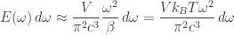$\displaystyle E(\omega) \, d \omega \approx \frac{V}{\pi^2 c^3} \frac{\omega^2}{\beta} \, d \omega = \frac{V k_B T \omega^2}{\pi^2 c^3} \, d \omega$ .

This is a form of the Rayleigh-Jeans law, which is the classical prediction for black body radiation. It’s approximately valid at low frequencies but becomes less and less accurate at higher frequencies.

Second, in the limit as $\beta \hbar \omega \to \infty$ (meaning low temperature relative to frequency), the denominator approaches $e^{\beta \hbar \omega}$ , and we get

$\displaystyle E(\omega) \, d \omega \approx \frac{V \hbar}{\pi^2 c^3} \frac{\omega^3}{e^{\beta \hbar \omega}} \, d \omega$ .

This is a form of the Wien approximation. It’s approximately valid at high frequencies but becomes less and less accurate at low frequencies.

Both of these limits historically preceded Planck’s law itself.

Wien’s displacement law

This form of Planck’s law is enough to tell us at what frequency the energy $E(\omega)$ is maximized given the temperature $T$ (and hence roughly what color a black body of temperature $T$ is): we differentiate with respect to $\omega$ and find that we need to solve

$\displaystyle \frac{d}{d \omega} \frac{\omega^3}{e^{\beta \hbar \omega} - 1} = 0$ .

or equivalently (taking the logarithmic derivative instead)

$\displaystyle \frac{3}{\omega} = \frac{\beta \hbar e^{\beta \hbar \omega}}{e^{\beta \hbar \omega} - 1}$ .

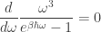Let $\zeta = \beta \hbar \omega$ , so that we can rewrite the equation as

$\displaystyle 3 = \frac{\zeta e^\zeta}{e^\zeta - 1}$

or, with some rearrangement,

$\displaystyle 3 - \zeta = 3e^{-\zeta}$ .

This form of the equation makes it relatively straightforward to show that there is a unique positive solution $\zeta = 2.821 \dots$ , and hence that $\beta \hbar \omega = \zeta$ , giving that the maximizing frequency is

$\displaystyle \boxed{ \omega_{max} = \frac{\zeta}{\beta \hbar} = \frac{\zeta k_B}{\hbar} T}$

where $T$ is the temperature. This is Wien’s displacement law for frequencies. Rewriting in terms of wavelengths $\ell = \frac{2 \pi c}{\omega}$ gives

$\displaystyle \frac{2 \pi c}{\omega_{max}} = \frac{2 \pi c \hbar}{\zeta k_B T} = \frac{b}{T}$

where

$\displaystyle b = \frac{2 \pi c \hbar}{\zeta k_B} \approx 5.100 \times 10^{-3} \, mK$

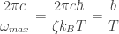
(the units here being meter-kelvins). This computation is typically done in a slightly different way, by first re-expressing the density of energies $E(\omega) \, d \omega$ in terms of wavelengths, then taking the maximum of the resulting density. Because $d \omega$ is proportional to $\frac{d \ell}{\ell^2}$ , this has the effect of changing the $\omega^3$ from earlier to an $\omega^5$ , so replaces $\zeta$ with the unique solution $\zeta'$ to

$\displaystyle 5 - \zeta' = 5 e^{-\zeta'}$

which is about $4.965$ . This gives a maximizing wavelength

$\displaystyle \boxed{ \ell_{max} = \frac{2 \pi c \hbar}{\zeta' k_B T} = \frac{b'}{T} }$

where

$\displaystyle b' = \frac{2 \pi c \hbar}{\zeta' k_B} \approx 2.898 \times 10^{-3} \, mK$ .

This is Wien’s displacement law for wavelengths. Note that $\ell_{max} \neq \frac{2 \pi c}{\omega_{max}}$ .

A wood fire has a temperature of around $1000 \, K$ (or around $700^{\circ}$ celsius), and substituting this in above produces wavelengths of

$\displaystyle \frac{2 \pi c}{\omega_{max}} = \frac{5.100 \times 10^{-3} \, mK}{1000 \, K} = 5.100 \times 10^{-6} \, m = 5100 \, nm$

and

$\displaystyle \ell_{max} = \frac{2.898 \times 10^{-3} \, mK}{1000 \, K} = 2.898 \times 10^{-6} \, m = 2898 \, nm$ .

For comparison, the wavelengths of visible light range between about $750 \, nm$ for red light and $380 \, nm$ for violet light. Both of these computations correctly suggest that most of the radiation from a wood fire is infrared; this is the radiation that’s heating you but not producing visible light.

By contrast, the temperature of the surface of the sun is about $5800 \, K$ , and substituting that in produces wavelengths

$\displaystyle \frac{2 \pi c}{\omega_{max}} = 879 \, nm$

and

$\displaystyle \ell_{max} = 500 \, nm$

which correctly suggests that the sun is emitting lots of light all around the visible spectrum (hence appears white). In some sense this argument is backwards: probably the visible spectrum evolved to be what it is because of the wide availability of light in the particular frequencies the sun emits the most.

Finally, a more sobering calculation. Nuclear explosions reach temperatures of around $10^7 \, K$ , comparable to the temperature of the interior of the sun. Substituting this in produces wavelengths of

$\displaystyle \frac{2 \pi c}{\omega_{max}} = 0.51 \, \mu m$

and

$\displaystyle \ell_{max} = 0.29 \, \mu m$ .

These are the wavelengths of X-rays. Planck’s law doesn’t just stop at the maximum, so nuclear explosions also produce even shorter wavelength radiation, namely gamma rays. This is solely the radiation a nuclear explosion produces because it is hot, as opposed to the radiation it produces because it is nuclear, such as neutron radiation.

http://qchu.wordpress.com/?p=25649

Extensions

https://qchu.wordpress.com/feed

Posts