Show full content
This year’s NCAA basketball tournament has just ended, which means a lot of people are currently cursing their bracket picks. That also means it’s a great time for a retrospective: How could one go about picking a better bracket? There are all kinds of considerations here, but in this post we’re going to focus on just one feature: team seedings.
In the NCAA tournament all 64 teams are placed in one of four regional tournaments, and the teams in each regional tournament are given seeds numbered 1 through 16. The regional tournaments are set up so that #1 seeds play #16 seeds, #2 seeds play #15 seeds, and so forth, for the first round. In the second round, the winner of 1 vs. 16 plays the winner of 8 vs. 9, the winner of 2 vs. 15 plays the winner of 7 vs. 10, and so on, continuing through four rounds. After the fourth round, fifteen teams from each region have been defeated, and the remaining team is the winner of the region and goes to the Final Four to play against the other regional winners.
The NCAA men’s tournament expanded to 64 teams in 1985. This gives us 40 years’ worth of information on how teams actually perform relative to their seeds. In this series of blog posts, we will use this information to investigate how you can improve your chances of winning your tournament bracket pool using information from the team seeds.
(For this purposes of this project, we are ignoring the play-in teams in the men’s tournament. Also, we will not include information from the NCAA women’s tournament, since the dynamics appear to be different: The top seeds and a small number of programs tend to dominate in a way that does not happen with the men’s tournament.)
Historical Winning PercentagesThe first thing to do is figure out the historical win rate for the various seed matchups. Kaggle’s Machine Learning Mania 2026 contains the all the data we need (much more than we need, in fact). We extract the data and keep only the yearly seed information from 1985 on, including which seeds won which matchups.
After all the data extraction, cleaning, and computation involved, we end up with a 16 x 16 matrix for seed vs. seed win/loss records from 1985 to 2025. The full matrix is given in the file below. A few details are worth pointing out.
First, the #1 seed has a winning record of 98.8% against the #16 seed. From 1985 to 2025, inclusive, there have been 40 NCAA tournaments (41 years less one for Covid-19), which means 160 games that have pitted a #1 seed against a #16. We know that a #16 seed has only won twice (UMBC over Virginia in 2018 and Fairleigh Dickinson over Purdue in 2023), giving a 158/160, or 98.75%, winning percentage for the #1 seed here. The 0.988 that appears in the table serves as a sanity check on our calculations.
In addition, several higher-numbered seeds have winning records against lower-numbered seeds (noted in orange). Many of these are based on only one or a few games, but one in particular is not. With 160 matchups, the #9 seeds actually have a winning record against the #8 seeds: 51.9%. There are also many, many seed vs. seed matchups that have never occurred in the tournament (noted in light yellow). Finally, several seeds have 100% winning records against particular other seeds (noted in light blue if not already colored orange). While historically accurate, these are based on only a few games and are suspicious from a modeling/analysis standpoint.
win_rate_matrixDownload Smoothing Winning Percentages with Bradley-TerryThe sparsity of the historical win rate matrix and the nonzero entries based on only few matchups are problems for us if we’re trying to do a full seed-vs-seed analysis. All is not lost, though: We can smooth the matrix in some fashion, using the historical information we do have to estimate the information we do not.
There are a few options available to us here, but perhaps the simplest robust choice is to use the Bradley-Terry model. In our terms, this model says that the probability that seed i defeats seed j in the tournament is

where 

Applying the Bradley-Terry model gives us the updated win-rate matrix below. This matrix looks much more reasonable: Every matchup has a win probability, and the probabilities seem reasonable (the #1 vs. #16 win rate of 98.8% is even preserved). The oddly high percentages below the diagonal have been smoothed out, leaving only three win rates in the orange, all of which seem plausible.
bt_win_rate_matrixDownloadNow, how do we use this model to pick a good bracket? We will continue the discussion in the next post, where we discuss how to maximize your expected bracket score.

 , but that’s generally not considered to be closed form. On the other hand, many modern programming languages like
  is, for a general probability model,
 is the survival function
  , and
, and  is the cumulative distribution function for the probability model.

 . Then
  .
. , this yields
  , so that
  . Then

 rather than
  to match the formulas given here.
 , is
, is  , as the vehicle will need to work fine for the first
  days (with probability
  for each day) and then break or crash on day k, with probability p. The probability that a vehicle will need to be replaced after n days is
  , as this is the probability that the vehicle will work fine for
  days. (It doesn’t matter whether it breaks on day n or not; it will still be replaced after day n.) Letting
  , the expected amount of time that a vehicle is in operation is thus (using the definition of expected value) given by
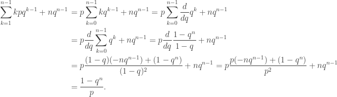
 as
as  and then swapping the order of summation. In the second line we use the geometric sum formula, and in the third line we use the quotient rule for derivatives.
 .
.  denote that claim that
  is true for some k; that is, suppose
  . Now,
  is the claim that
  . If
. If  , which proves that the truth of
  , all people in a group of size n share the same birthday.
 is true, as all people in a group of size 1 have the same birthday. Now, suppose that
  people. Single out one of those people; perhaps his name is Al. Without Al, we have a group of k people, all of whom must, by our inductive hypothesis, share the same birthday. Now, swap Al with one of those other k people. Now Al is in a group of k people. Again, by hypothesis all of them must share the same birthday. So Al must have the same birthday as all the others in his group. Thus these
  , and we remove Al from the group of two people, we then have Al and a group of size 1. Swapping Al with that one other person does put Al in a group of size 1, and he does share the same birthday as everyone else in the group (namely, just himself), but he doesn’t necessarily share the same birthday with that one other person. So
  , even though
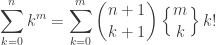
  , together with combinatorial proofs of two formulas for this power sum. (An earlier version of some of the results in this paper actually appeared in a
 ![f: [m+1] \mapsto [n+1]](https://s0.wp.com/latex.php?latex=f%3A+%5Bm%2B1%5D+%5Cmapsto+%5Bn%2B1%5D&bg=ffffff&fg=333333&s=0&c=20201002) such that, for all
such that, for all ![i \in [m]](https://s0.wp.com/latex.php?latex=i+%5Cin+%5Bm%5D&bg=ffffff&fg=333333&s=0&c=20201002) ,
,  .
. this doesn’t work. The power sum as I stated it entails adding up n copies of 1 and so evaluates to n. On the other hand, the set
 ![[m]](https://s0.wp.com/latex.php?latex=%5Bm%5D&bg=ffffff&fg=333333&s=0&c=20201002) is the set
is the set  . This means that all
  functions from
 ![[1]](https://s0.wp.com/latex.php?latex=%5B1%5D&bg=ffffff&fg=333333&s=0&c=20201002) to
to ![[n+1]](https://s0.wp.com/latex.php?latex=%5Bn%2B1%5D&bg=ffffff&fg=333333&s=0&c=20201002) vacuously satisfy the condition in the theorem. The theorem as stated in the paper is off by 1, then, for the case
vacuously satisfy the condition in the theorem. The theorem as stated in the paper is off by 1, then, for the case  , so that we have the following.
 is the number of functions
  (and I am a fan of this convention in a combinatorial setting), this allows the formula to hold in the case
 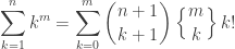 , and
, and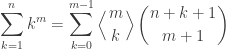 .
. , and
, and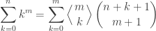 .
. . The definition for

 can be expressed as
  , for complex numbers s whose real part is greater than 1. By analytic continuation,
  .
.  is given by
  . (Sometimes M is given as the upper bound, but for this post it’s more convenient to use
  .)
.) and the power sum
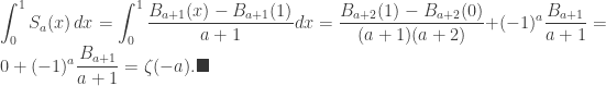
  . It’s due to Mináč [1], and I reproduce his proof here.
 .
. from 0 to 1? Well, it’s also known that
  in M. For example,
 .
. .
. .
. ) are 0.
 .
.

 for the left-hand side and
  for the right-hand side. Since the first constraint is an equality and the second is an inequality, this implies
 , it’s also true that
  , and so
 and
and  to force

 and
and  variables separately. First, we need the total
  .
. . Since
  .
.
 .
. .
.
 .
. , the function that counts the number of divisors of an integer:
 .
. , where p is prime. Since the only divisors of
  , the number of divisors of
  .
. . We have
 and
and 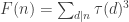 . What we’ve shown thus far is that
  .
.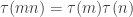 when m and n are relatively prime. This is one of the first properties you learn about
  is multiplicative.
  is also multiplicative. This is a special case of the more general result that the
  , take h to be the identity function; i.e.,
  .) This means that our functions f and F defined in the previous paragraph are both multiplicative.
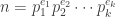 , we have
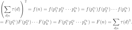

 are called
  has no integer solutions, using (with one exception) nothing more complicated than congruences.
 ,
,  . Looking at the equation modulo 8, then, we have
 .
. and reduce them modulo 8 we have
  . So there is no integer y that when squared is congruent to 7 modulo 8. Therefore, there is no solution to
  or
or  .
. . However, if we square the residues
  and reduce them modulo 4 we get
  . So there is no integer y that when squared is congruent to 2 modulo 4. Thus there is no solution to
  when
when  .
. . If
. If  has prime factors that are all equivalent to 1 modulo 4, then their product (i.e.,
  ) would be equivalent to 1 modulo 4. Thus
  , then
  . This means that
  . However, thanks to
  can have a solution to
  ,
,