Show full content
This post introduces a project that Gabriel Desfrene did in my group as an intern last summer. Gabriel will present his project in a paper coauthored with my PhD students Quentin Corradi and Michalis Pardalos and myself at CAV 2026 in July.
Verilog (aka SystemVerilog) is the most widely used language for specifying, designing, and verifying all kinds of computer hardware. But some aspects of the language are widely misunderstood – even some as fundamental as “how many bits are used for each operation”.
Consider this example, which is due to Quentin:
logic [3:0] foo;
assign foo = (3'b110 + 3'b110 + 3'b110 + 3'b110) >> 2;
The first line is declaring foo to be a 4-bit variable. On the second line, 3'b110 is Verilog for “the 3-bit binary number 110”, and >> is the right-shift operation. That is, we are performing the addition of four copies of 110, then shifting to the right by 2, and finally storing the result in foo.
Verilog is a hardware description language: it describes pieces of hardware. This means that the addition written in Verilog has to map to a physical “adder” in the eventual hardware. And in order for that adder to come into being, it must have a width.
But what is the correct width?
- Option 1. We could use a 3-bit adder – the same width as the operands. Then
110+110+110+110gives000(it would have been11000, but the highest two bits are lost to overflow). And after the right-shift we get000. Thus, the final value offoo, after adding a leading zero to make a 4-bit value, is0000. - Option 2. Perhaps we should use a wider adder? This would have the advantage of not losing bits to overflow, but the disadvantage of requiring more circuitry (which leads to hardware that ultimately consumes more electricity). If we don’t want to lose any bits to overflow here, we need at least a 5-bit adder. Then
110+110+110+110gives11000, and after the right-shift we get00110. Thus, the final value offoo, after chopping off the leading zero to make a 4-bit value, is0110.
Which of these options does the Verilog language standard say is the correct one? Well, it actually opts for Option 3: the width of the adder is, in fact, determined by the width of the variable being assigned to (i.e. foo) which is 4 bits in our example. So the addition 110+110+110+110 gives 1000 (losing just one bit to overflow this time), and after the right-shift we get 0010 as the final value for foo.
Examples like this are a well-known source of confusion among hardware engineers. For instance, a fairly well established Verilog tutorial from ChipVerify.com quite reasonably warns its readers that “[calculating the bitwidths of expressions] is subtle”.
It then goes on to get the explanation completely wrong. It incorrectly states that if a and b are 8-bit variables, then “assign product = a * b” will “lose the upper bits of the actual 16-bit product”, even if product has 16 bits. (In fact, this multiplication happens at 16 bits, that being the width of the left-hand side of the assignment, so no bits are lost to overflow.)
I asked Reddit’s resident Verilog experts about ChipVerify’s example. They unanimously (at the time of writing) described the tutorial as incorrect.
But they all gave different reasons as to why it is incorrect.
And none of those reasons were right.
Still, as Bill Vaughan famously wrote, “To err is human; to really foul things up requires a computer.” So, let’s see whether today’s AI models understand Verilog’s bitwidth rules any better than those humans do. Here’s what ChatGPT said when I asked it what value gets assigned to foo in my example:
Each operand is a 3-bit value (
3'b110= 6). In SystemVerilog, when you add fixed-width vectors, the result does not automatically grow—it stays the width of the operands unless you explicitly widen it. So each intermediate addition is truncated back to 3 bits [and] the full sum becomes3'b000. […] Finally, assigning tologic [3:0] foozero-extends the result:foo = 4'b0000(decimal 0).
In other words, it’s going for Option 1. This is wrong.
Meanwhile, Meta’s Muse Spark model goes for Option 2, which is also wrong:
In SystemVerilog, when you add unsigned values, the result width is
max(widths) + 1for each addition. […] Result:foo = 4'b0110= 6 decimal. Key gotcha: If you thought the 3-bit operands would truncate the sum at each step, they don’t. Verilog/SystemVerilog expands the width during expression evaluation. The truncation only happens on the final assignment to the 4-bitfoo, but 6 fits fine.
Claude Opus 4.1 also goes for Option 2 to begin with, but then it changes its mind mid-response, and ends up going for the correct Option 3:
The value assigned to
foois 6 (binary0110). […] Wait—that’s not quite right either. Let me reconsider the expression context. […] Hmm, but there’s more nuance—the3'b110literals are explicitly 3-bit, and the intermediate width depends on how operands combine. […] Since the final assignment target is 4-bitfoo, the entire expression is context-determined to 4 bits. […] Final answer:foo = 4'b0010(decimal 2).
Google’s Gemini is the only model I tried that confidently gets it right first time:
In SystemVerilog, the bit-width of an expression is determined by the “context-determined” rules. Since
foois a 4-bit logic type, the entire right-hand side is evaluated using 4-bit precision. […] The value assigned tofoois4'b0010(decimal 2).
Anyway, the long and short of it is this: Verilog’s rules for bitwidths are confusing.
To some extent, the rules are unavoidably complicated, but a large part of the problem is that they are specified in informal prose that is spread over several parts of the (very large) Verilog standard.
So, aiming to bring as much clarity as possible to the situation, we decided to formalise Verilog’s rules for bitwidths in the Rocq theorem prover. The murky details are in our paper and in Gabriel’s Rocq development, but in this blog post I’ll just explain how things work roughly, via a few examples.
The calculation happens in two stages. These stages are called “determine” and “propagate”. In the “determine” phase, bitwidth information flows up the expression tree, calculating the “self-determined width” of every sub-expression. Then, in the “propagate” phase, bitwidth information flows back down the expression tree, fixing the “final width” of every sub-expression.
Here’s how it works on our example. We start with the expression we want to analyse, drawn as a syntax tree:

The addition is labelled as just a “BinOp” (binary operation) because all arithmetic operations (additions, subtractions, multiplications, and so on) are handled in the same way. The only node that has a bitwidth already is foo, and that bitwidth is obtained from foo‘s declaration.
The “determine” phase sends bitwidth information up this tree, as shown by the red arrows in the following picture:

Working from the bottom, we see that the constants all have a self-determined width of 3, and this fixes the self-determined width of the BinOp at 3 too (3 being the max of 3, 3, 3, and 3). Thus the ShiftOp also has a self-determined width of 3 (it ignores the width of its right-hand operand). The width of the top-level assignment operation is determined only by its left-hand operand, foo, which has a width of 4.
Then, the “propagate” phase sends bitwidth information back down the tree. In the following picture, we write “ShiftOp : 3 → 4” to mean that the self-determined width of the ShiftOp is 3, but its final width is 4.

Thus, we can see that the final width of the adder (the BinOp in the middle of the picture above) is 4 bits.
For the example from ChipVerify’s tutorial, the “determine” phase sets the self-determined width of the multiplication to be 8 bits, but the “propagate” phase sets its final width to 16 bits because this is the width of the left-hand side of the assignment.
I’ll do one last example, as there’s one more subtlety that is worth mentioning. Consider another little Verilog design:
logic [3:0] baz;
assign baz = (3'b110 + {2'b10, 1'b0}) >> 2;
It’s similar to our first example, but it includes a concatenation operation, in which the 2 bits of 2'b11 are placed alongside the single bit of 1'b0 to form the 3-bit value 3'b100. Drawn as a syntax tree, we have:

After running the “determine” phase, we get:

Note that the self-determined width of the concatenation operation is the sum (+) of the widths of its operands. The rest is similar to the previous example.
The difference comes when we run the “propagate” phase:

Note that the width of 4 has propagated from baz, setting the final width of the shift, the BinOp, the constant 3'b110, and the concatenation. But it has not propagated below the concatenation. The concatenation operation can thus be seen as a “boundary” to propagation. In the terminology of the Verilog standard, each operands of a concatenation operation has its bitwidth “solely determined by the expression itself” and not “by the fact that it is part of another expression”.
So there we go; that’s more-or-less how bitwidth calculations really work in Verilog. Our paper has more of the details, and more still are available in Gabriel’s Rocq development. We imagine that our work can be valuable in a couple of ways. Firstly, we expect that it can strengthen the guarantees provided by tools like Lustig and Vera, which can reason formally about the correctness about Verilog designs but currently have to assume that all bitwidths have been written out explicitly. Secondly, we hope that our work can help the maintainers of the Verilog standard come up with a way to explain bitwidth calculations with more clarity and precision, so as to minimise confusion in the future.


 and
and  when giving a semantics to Hoare triples. In response to that post,
 to mean that if command
  is started in state
  it can produce final state
  . Our commands need not always terminate: if there is no
  with
with  , then that means
  is that whenever
  (an assertion is just a set of states), any final state it reaches must satisfy the assertion
  . That is…
 .
. for the set of all states that command
  .
. to give a semantics to Hoare triples in a variety of different ways. For instance, the partial correctness interpretation given above can be rewritten as…
 .
.
 (a backward semantics).
 may
may may
may must
must must
must must
must must
must if we define
  as the “weakest liberal precondition” in the usual way…

 .
.
 and
and  .
. between triples such that the triple
  holds according to the other semantics. What this means is that one strategy for proving
  ) is equivalent to
  ) because…
 that maps
  .
. ) is equivalent to
  ) because, using another bijection
  that maps
  , we have…
 .
. and
and  and
and  , but it could become infeasible in more complicated settings. Likewise, the bijection
  ), which is fine in ordinary predicate logic but doesn’t work very nicely in a substructural logic like separation logic.


 .
.
 . Another way is to introduce the concept of a strongest postcondition, also due to Dijkstra, like so:
 .
.![[P]\,c\,[Q]](https://s0.wp.com/latex.php?latex=%5BP%5D%5C%2Cc%5C%2C%5BQ%5D&bg=ffffff&fg=404040&s=0&c=20201002) that have a subtly different meaning to Hoare’s, namely:
that have a subtly different meaning to Hoare’s, namely: .
.
 is not the same as
  , which shall mean:
 .
.
 triples? What properties do they enjoy?
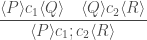
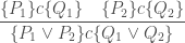
![\displaystyle\frac{ [ P ] c_1 [ Q ] \quad [ Q ] c_2 [ R ] } { [ P ] c_1 ; c_2 [ R ] }](https://s0.wp.com/latex.php?latex=%5Cdisplaystyle%5Cfrac%7B+%5B+P+%5D+c_1+%5B+Q+%5D+%5Cquad+%5B+Q+%5D+c_2+%5B+R+%5D+%7D+%7B+%5B+P+%5D+c_1+%3B+c_2+%5B+R+%5D+%7D&bg=ffffff&fg=404040&s=0&c=20201002)

![\displaystyle\frac{ [ P ] c [ P ] } { [ P ] c^* [ P ] }](https://s0.wp.com/latex.php?latex=%5Cdisplaystyle%5Cfrac%7B+%5B+P+%5D+c+%5B+P+%5D+%7D+%7B+%5B+P+%5D+c%5E%2A+%5B+P+%5D+%7D&bg=ffffff&fg=404040&s=0&c=20201002)


![\displaystyle\frac{ Q \Rightarrow P } { [ P ] \text{skip} [ Q ] }](https://s0.wp.com/latex.php?latex=%5Cdisplaystyle%5Cfrac%7B+Q+%5CRightarrow+P+%7D+%7B+%5B+P+%5D+%5Ctext%7Bskip%7D+%5B+Q+%5D+%7D&bg=ffffff&fg=404040&s=0&c=20201002)

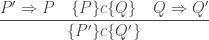
![\displaystyle\frac{ P \Rightarrow P' \quad [ P ] c [ Q ] \quad Q' \Rightarrow Q } { [ P' ] c [ Q' ] }](https://s0.wp.com/latex.php?latex=%5Cdisplaystyle%5Cfrac%7B+P+%5CRightarrow+P%27+%5Cquad+%5B+P+%5D+c+%5B+Q+%5D+%5Cquad+Q%27+%5CRightarrow+Q+%7D+%7B+%5B+P%27+%5D+c+%5B+Q%27+%5D+%7D&bg=ffffff&fg=404040&s=0&c=20201002)

 that always diverges (fails to terminate):
 always holds, because Hoare logic gives no guarantees about non-terminating executions.
![[ P ] \varnothing [ Q ]](https://s0.wp.com/latex.php?latex=%5B+P+%5D+%5Cvarnothing+%5B+Q+%5D&bg=ffffff&fg=404040&s=0&c=20201002) holds iff
holds iff  , because Incorrectness logic demands termination.
 holds iff
  , because
  be the set of states from which execution of
  holds iff
  ; i.e.
 ![[ P ] c [ False ]](https://s0.wp.com/latex.php?latex=%5B+P+%5D+c+%5B+False+%5D&bg=ffffff&fg=404040&s=0&c=20201002) always holds.
always holds. holds iff
 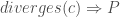 ; i.e.
  , which denotes a non-deterministic choice between commands
  and
and  :
: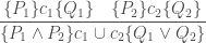
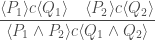
![\displaystyle\frac{ [ P_1 ] c_1 [ Q_1 ] \quad [ P_2 ] c_2 [ Q_2 ] } { [ P_1 \vee P_2 ] c_1 \cup c_2 [ Q_1 \vee Q_2 ] }](https://s0.wp.com/latex.php?latex=%5Cdisplaystyle%5Cfrac%7B+%5B+P_1+%5D+c_1+%5B+Q_1+%5D+%5Cquad+%5B+P_2+%5D+c_2+%5B+Q_2+%5D+%7D+%7B+%5B+P_1+%5Cvee+P_2+%5D+c_1+%5Ccup+c_2+%5B+Q_1+%5Cvee+Q_2+%5D+%7D&bg=ffffff&fg=404040&s=0&c=20201002)
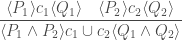

![\displaystyle\frac{ [ P_1 ] c [ Q_1 ] \quad [ P_2 ] c [ Q_2 ] } { [ P_1 \vee P_2 ] c [ Q_1 \wedge Q_2 ] }](https://s0.wp.com/latex.php?latex=%5Cdisplaystyle%5Cfrac%7B+%5B+P_1+%5D+c+%5B+Q_1+%5D+%5Cquad+%5B+P_2+%5D+c+%5B+Q_2+%5D+%7D+%7B+%5B+P_1+%5Cvee+P_2+%5D+c+%5B+Q_1+%5Cwedge+Q_2+%5D+%7D&bg=ffffff&fg=404040&s=0&c=20201002)
 be the set of states from which execution of
  then
then  implies
 ![[Q] c^{-1} [P]](https://s0.wp.com/latex.php?latex=%5BQ%5D+c%5E%7B-1%7D+%5BP%5D&bg=ffffff&fg=404040&s=0&c=20201002) .
. then
then  .
. ” command like so:
![[ x = n ] \, {+}{+}x \, [ x = n + 1 ]](https://s0.wp.com/latex.php?latex=%5B+x+%3D+n+%5D+%5C%2C+%7B%2B%7D%7B%2B%7Dx+%5C%2C+%5B+x+%3D+n+%2B+1+%5D&bg=ffffff&fg=404040&s=0&c=20201002)


![[ x > n ] \, {+}{+}x \, [ x > n + 1 ]](https://s0.wp.com/latex.php?latex=%5B+x+%3E+n+%5D+%5C%2C+%7B%2B%7D%7B%2B%7Dx+%5C%2C+%5B+x+%3E+n+%2B+1+%5D&bg=ffffff&fg=404040&s=0&c=20201002)


![[ x > 2 ] \, x := 5 \, [ x = 5 ]](https://s0.wp.com/latex.php?latex=%5B+x+%3E+2+%5D+%5C%2C+x+%3A%3D+5+%5C%2C+%5B+x+%3D+5+%5D&bg=ffffff&fg=404040&s=0&c=20201002)
 is invalid because
  is not necessary to guarantee
  after the assignment. In fact, any initial state will suffice here, which means
  is valid.
![[ x > 2 ] \, x := 5 \, [ x > 3 ]](https://s0.wp.com/latex.php?latex=%5B+x+%3E+2+%5D+%5C%2C+x+%3A%3D+5+%5C%2C+%5B+x+%3E+3+%5D&bg=ffffff&fg=404040&s=0&c=20201002) is invalid because executing
is invalid because executing  can never reach a final state where
  , say. And
 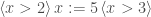 is invalid too, for the same reason as given above.
![[ True ] \, (x := 4) \cup (x := 5) \, [ x = 4 \vee x = 5 ]](https://s0.wp.com/latex.php?latex=%5B+True+%5D+%5C%2C+%28x+%3A%3D+4%29+%5Ccup+%28x+%3A%3D+5%29+%5C%2C+%5B+x+%3D+4+%5Cvee+x+%3D+5+%5D&bg=ffffff&fg=404040&s=0&c=20201002)


![[ x > n ] \, ({+}{+}x) \cup \text{skip} \, [ x > n ]](https://s0.wp.com/latex.php?latex=%5B+x+%3E+n+%5D+%5C%2C+%28%7B%2B%7D%7B%2B%7Dx%29+%5Ccup+%5Ctext%7Bskip%7D+%5C%2C+%5B+x+%3E+n+%5D&bg=ffffff&fg=404040&s=0&c=20201002)

 triples.


 ,
,  , and
, and  .
. 
 and
and  .
.
 function), but no numbers are both odd and even. The analogy between odd/even functions and odd/even numbers simply does not work at all.


 On the other hand, if we try to draw this diagram in the “action-oriented” style, it becomes tricky to deal with pieces of data that are consumed or produced by multiple actions, such as the “IR” data in the picture below.


