https://jacco.ompf2.com/feed

Recently we (BUas colleague Peter van Dranen and me) released a 3D racing game for the MSX2 retro platform: A 1986 Z80-based home computer standard, supported by all major manufacturers at the time, including Philips, Sony, JVC, Toshiba and Panasonic.

MSX2 is normally not a platform on which one would render 3D graphics. This was the time of the ZX-Spectrum and the Commodore 64, and graphics were tile-based, with additionally (at least on C64 and MSX) hardware sprite support.

That being said, some 3D games did exist. For example, David Braben’s Elite runs well on the platform, if the player is willing to accept a frame rate of about 5 fps, as well as wireframe 3D objects.

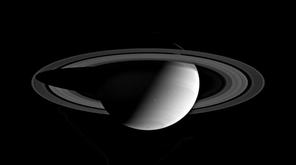
Also worth mentioning is Konami’s Penguin Adventure, which used some clever tricks to produce quite convincing 3D.

Still, it seems rather far-fetched to even attempt an action game with full-screen polygon graphics. And in fact it is! However, learning from Konami, and taking advantage of some specific features of the platform, we can produce something that convinces the player that this appears to be precisely what we did.

In this article we describe the renderer of DELTA (a.k.a. “Dodge! Engage! Launch! Target! Assault!”). We start with a description of the MSX2 platform specifics relevant to the technique. We then show that 3D images of reasonable complexity can be encoded as tiles and sprites. And finally, we show how this data can be compressed to better fit available ROM options, while allowing for fast run-time decompression.

Platform Specifics: VDP

The MSX2 platform provides graphics via its VDP (Video Display Processor), specifically: the V9938. The chip provides several display modes, including a full-colour 256×192 mode and a 16-color 512×192 mode. The modes that offer most freedom are of course also those that require most bandwidth, which makes them often impractical for real-time graphics.

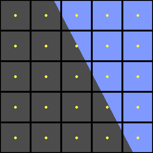
Promising are the tile-based modes, which use 8×8 character tiles to fill the screen. Each tile uses a byte per line of 8 pixels to define its ‘pattern’, as well as a byte per line to define the two colors used in that pattern. This way a tile requires only 16 bytes of storage, while allowing the use of 16 colours, as long as no more than two colours per line of 8 pixels are used. Tiles often don’t change from frame to frame, which further reduces required bandwidth. Instead, the tile based screen modes use a ‘name table’ of 768 bytes which index the 256 unique tiles.

The screenshot of Gradius 2 shows this approach in action. Colourful tiles are used (and re-used) to build a detailed display. Scrolling happens with 8 pixels at a time, and is done by modifying the name table alone.

Gradius 2 also shows another important feature of the MSX2 VDP: Hardware sprites. The player ship, bullets and smaller enemies are rendered using 8×8 or 16×16 images. A maximum number of 32 of these can be displayed at any time, on top of the tile display. There is a limitation however: Each screen line can display a maximum of 8 sprites at a time. These sprites will turn out to be very useful for solving the ‘two colours per 8 pixels’ limitation of the tiles.

Platform Specifics: Memory

Apart from the VDP there is another important (and rather unique) aspect of the MSX2 hardware standard: Memory. Where other systems at the time were limited to 64 kilobytes or 128 kilobytes, MSX2 went above and beyond.

The 64KB limitation is a result of the choice of processor: The Z80 (like other common CPUs at the time) can only use 16 bits for RAM addresses, which limits RAM to 65536 bytes. MSX2 however solves this with various mechanisms (slots, memory mappers, megaroms), effectively doing away with any and all limits on RAM and ROM capacity. Back in 1988 this allowed Konami to use 4 Megabit (512KB) for Metal Gear 2 Solid Snake; however in 2025 the community is producing Flash cartridges of up to 16MB. On top of that, all that memory can be accessed at the same speed: The CPU will never know the difference between the original 64KB and the expanded 16MB. This opens up entirely new ways of doing graphics.

Numbers

Before we dive into the specifics of the DELTA renderer, let’s list some numbers that affect what can and cannot be done.

CPU: Zilog Z80A, running at 3.58Mhz. It needs four cycles per instruction, at least. At 20 fps, the very best it can do is 179,000 instructions. In practice, it will do far less. The CPU can (at best) copy bytes at a rate of 1 per 5.5 cycles, so ~651KB per second or 32.5KB per frame at 20fps.

VDP: Data transfer to the VDP is slower. The details are complex, but in general, the VDP cannot accept data faster than 1 byte per 15 cycles, or ~12KB per frame at 20fps.

Bandwidth: The bandwidth-friendly tile-based mode ‘GRAPHIC4’ (see below) displays 32×24=768 tiles. The name table stores a byte for each of these, so changing each tile index requires writing 768 bytes. If we also want to update the tiles themselves, we need to write 16 bytes per tile for patterns and colours, so 4KB in total. And finally, if we want to update the patterns for 32 sprites of 16×16 pixels, we need to write 1KB of data. The colours for those sprites sum up to 512 bytes, and their position and index data is another 128 bytes. It sounds like a lot, but when we sum everything, it turns out that we can update everything that affects screen appearance by writing 6,528 bytes, i.e. well within the bandwidth limit of the VDP.

Data: For a racing game we need a track of some length. At 20fps, 800 frames yield a 40 second race; two laps make this 1 minute and 20 seconds, which seems about right. At 6,528 bytes per frame, this would be a little more than 5.2MB.

The DELTA Renderer

With the above in mind, our goal now becomes to convert a 256×192 16-color bitmap to (no more than) 256 tiles, plus a 32×24 name table indexing those tiles, and a set of sprites. A ‘nice to have’ would be some form of compression, so a 16MB cartridge can store at least 4 (but ideally more) tracks.

The question is of course, will 256 unique tiles be sufficient for all frames of the track, and how many sprites will we need to resolve issues where 8 pixels on a tile need more than 2 colours?

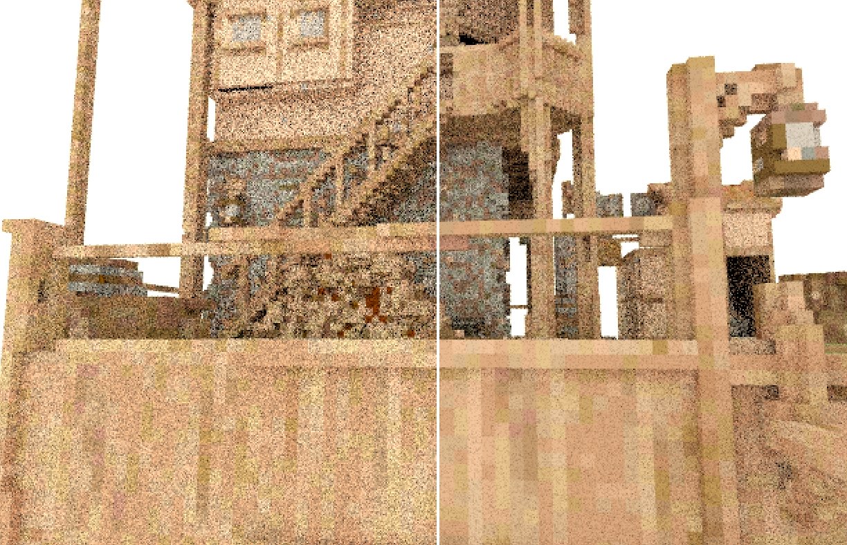
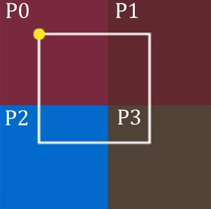
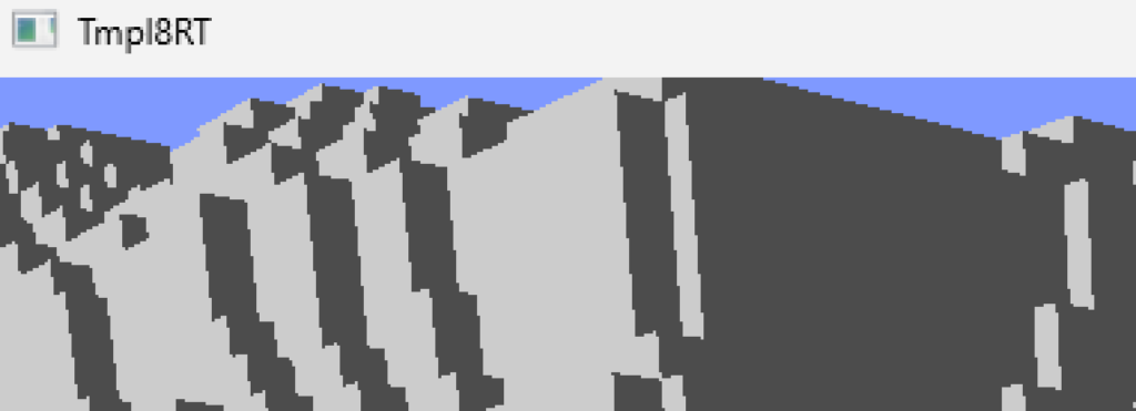
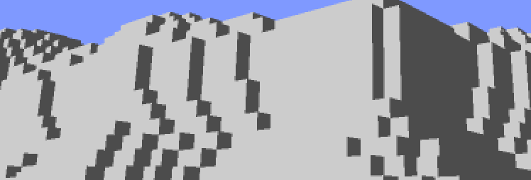
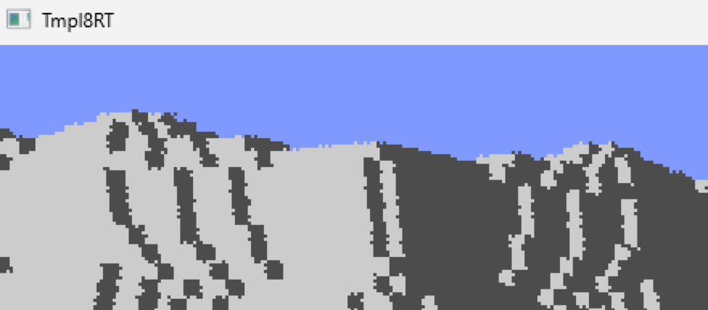
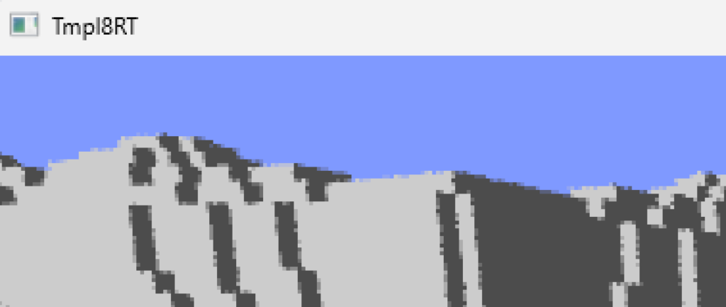
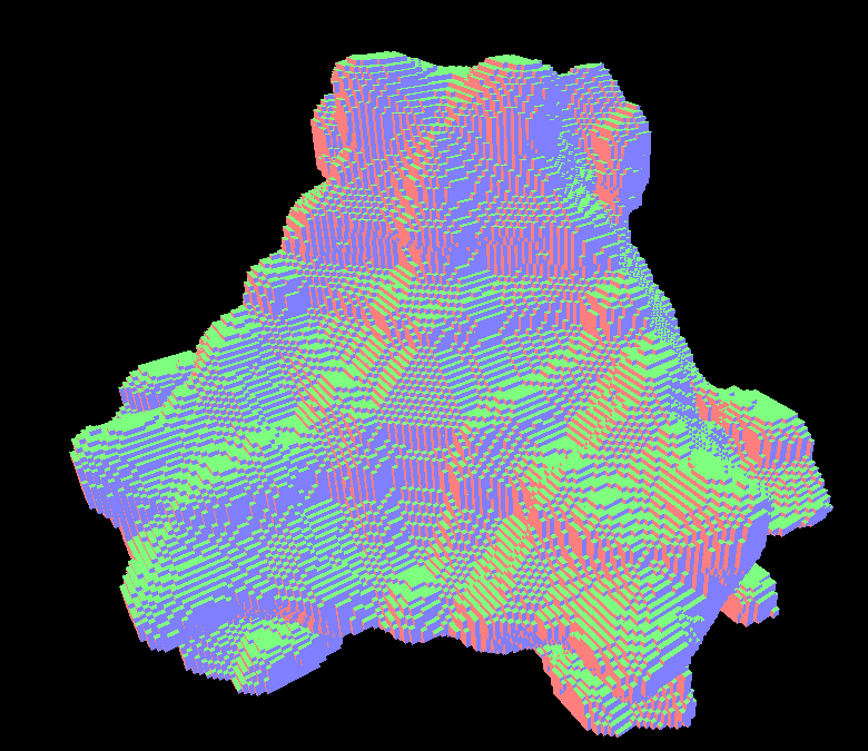
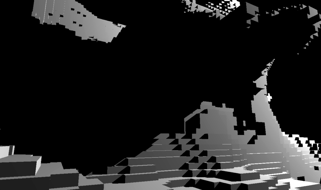
Here is a frame from the game (on the left) with the (not yet repaired) tiles on the right:

The tiles used in this frame are:

This is well within budget; in fact 31 tiles remain unused for this frame, some of which are claimed for displaying score and other game data. It turns out that this is the case for all frames of the animation: As long as the detail is dosed carefully, it is quite possible to make a pleasing 3D environment using just 236 or so tiles.

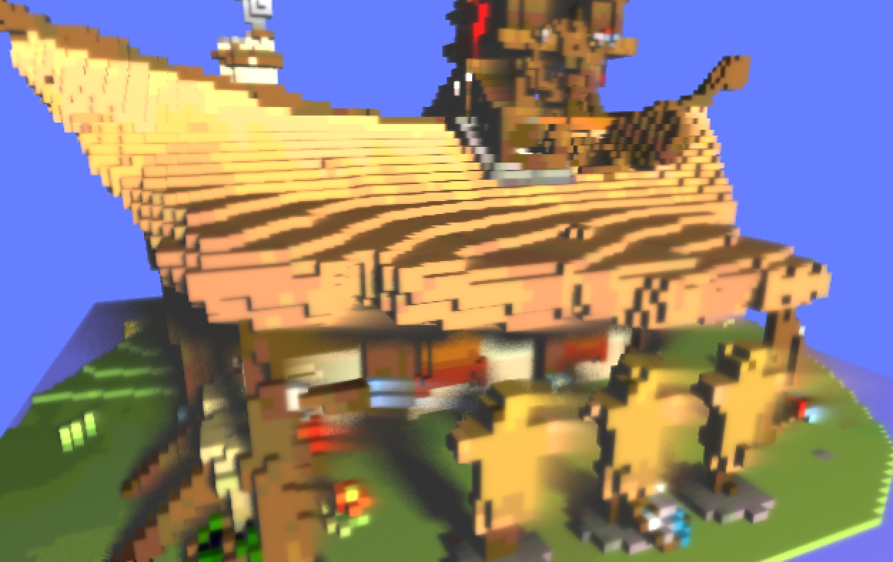
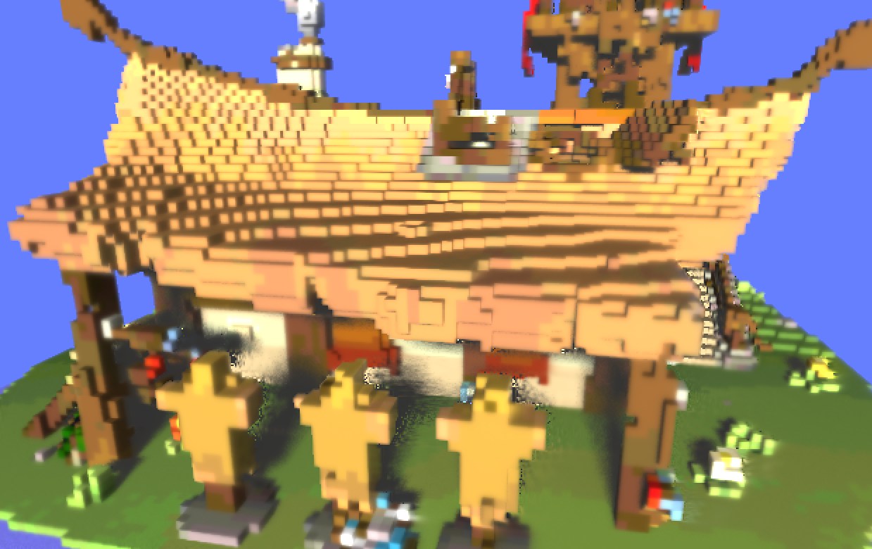
The sprite set needed to resolve the remaining issues is modest as well:

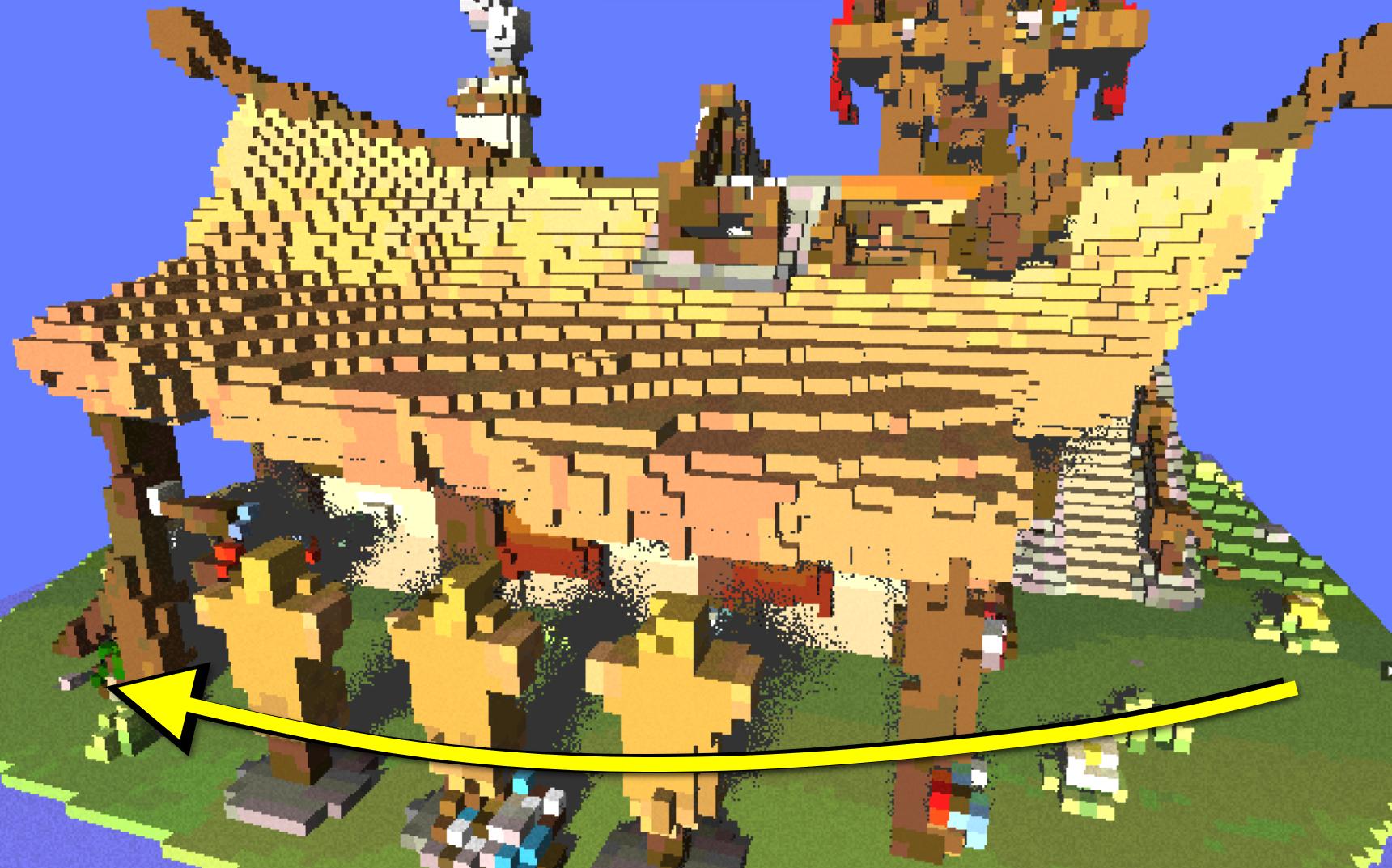
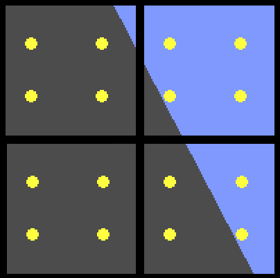
Note how e.g. the yellow sprites above the car resolve the problem where a single tile must display blue for the water, dark-grey for the track and yellow for the speed lane symbols.

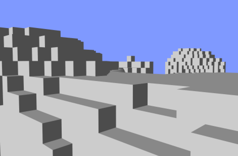
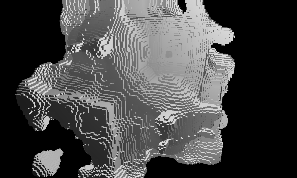
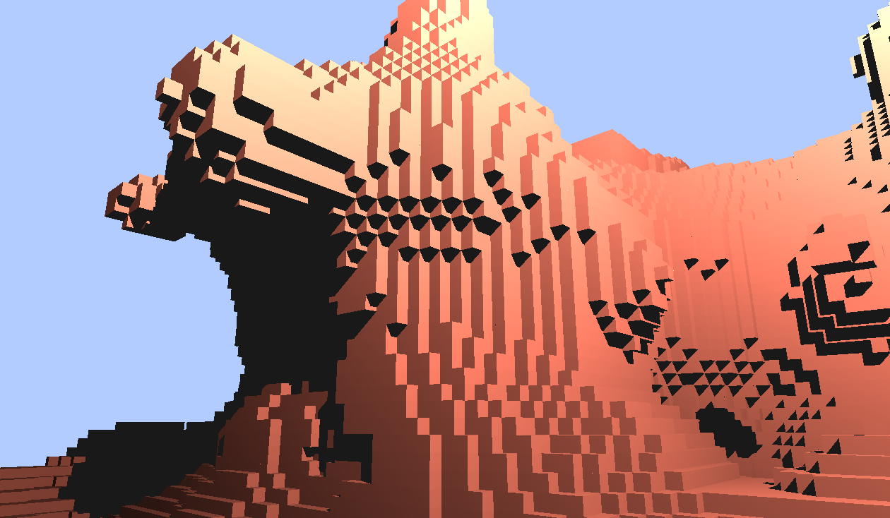
Some frames are more complex. For example, this frame from the intro animation:

Here, the subtle shading on the letters M and S causes substantial issues for the tile conversion. A lot of sprites are needed to remedy this:

So many in fact that we run the risk of exceeding the 8 sprites per line limit. This limit is strict on MSX2: Even parts of the sprite that do not contain any pixels contribute to the count, and exceeding the limit makes sprites invisible, exposing the tile issues we where trying to hide.

Luckily, most ‘remedial sprites’ do not use the full 16×16 square available to them. By shifting the set pixels up or down it is often possible to find a sprite configuration where no line contains more than 8 sprites.

During gameplay this challenge is even greater however, and this is where DELTA occasionally fails. The car sprite needs multiple colours, and therefore multiple sprite layers. It is also larger than 16×16 for many angles, and therefore the car is rendered using no less than 8 sprites. These do not occupy the same lines on-screen, but still four sprites do – and that means the scenery has only four slots to work with, at least on the screen lines occupied by the player car. One consequence of this is that DELTA is strictly a single-player game, without other cars to combat the player.

GRAPHIC4

In the next section we will discuss how the prerendered data can be compressed. Before we get to that, we look at the used VDP mode in some more detail.

Mirror Mode

GRAPHIC4 on the MSX2 VDP refers to a 16-color tiled video mode, where each of the 16 colours can be chosen from a 9-bit palette. On top of the tiles, up to 32 single-color sprites can be displayed, with a maximum of 8 occupying any screen line.

Tile indices are stored in a 768 byte (i.e., 32×24) name table. By default, GRAPHIC4 uses three tile sets: One for the top 1/3rd of the screen, one for tile lines 9 – 15 and the final one for tile lines 16 – 23, effectively allowing a unique tile on every location, if desired. Mirror mode allows these three sets to be identical, so that a tile used on position (0,0) can also be used on tile position (0,8). DELTA uses this mode to reduce tile data from 3x 4KB to 1x 4KB.

VRAM Layout

The MSX2 VDP lets the programmer select where each of the data tables is located in VRAM. The tables are:

• Name table: Stores tile indices. 768 bytes, by default located at 0x1800.
• Tile pattern data: 256 x 8 = 2048 bytes, by default located at 0x0000.
• Tile colour data: 256 x 8 = 2048 bytes, by default located at 0x2000.
• Sprite pattern data: 32 x 32 = 1024 bytes, by default located at 0x3800.
• Sprite colour data: 32 x 16 = 512 bytes, by default located at 0x1C00.
• Sprite attribute data: 32 x 4 = 128 bytes, by default located at 0x1E00.

DELTA renders at 20fps and thus needs 3 NTSC frames to create the next image. This means that double buffering is required. In the case of DELTA, this means: double-buffering all tables. We use the following layout:

TablePage 0Page 1Name Table0x18000x2800Tile Patterns0x00000x4000Tile Colours0x20000x6000Sprite Patterns0x08000x3800Sprite Colours0x1C000x2C00Sprite Attributes0x1E000x2E00

Switching between the two pages is very fast and can be done during the vertical retrace to avoid tearing.

Note that in the above scheme, only 64KB is used, which simplifies setting VRAM addresses somewhat. Moreover, the name table and sprite data for both pages resides within the first 16KB, further reducing the effort of specifying VRAM addresses. Only the tile patterns and colours touch addresses above 0x4000; these are however always written in large batches, amortizing the VRAM address setup cost over many writes.

Compression

In the previous sections we discussed the specifics of the MSX2 video processor. Respecting the limitations of the system, but ignoring ROM size for the moment, we conclude the hardware meets our initial requirements:

• We can convert 16-color images containing reasonable polygon detail to less than 256 tiles.
• The number of sprites needed to remedy tile colour issues is reasonable.
• Bandwidth is within boundaries.

However, even when we do not use all tiles for all frames, the raw data for 800 animation frames approaches 5MB, which is unwieldy. So, a new question arises: Can this data be compressed, and can the poor Z80 decompress it fast enough to make this worthwhile?

We approach this question in three steps:

1. Reducing per-frame sprite data traffic
2. Optimal run-length encoding and decoding of tile colour data
3. Run-length encoding of tile pattern data
4. Adaptive run-length encoding of the name table data
5. Data placement in megarom segments

Each step is detailed in the following paragraphs.

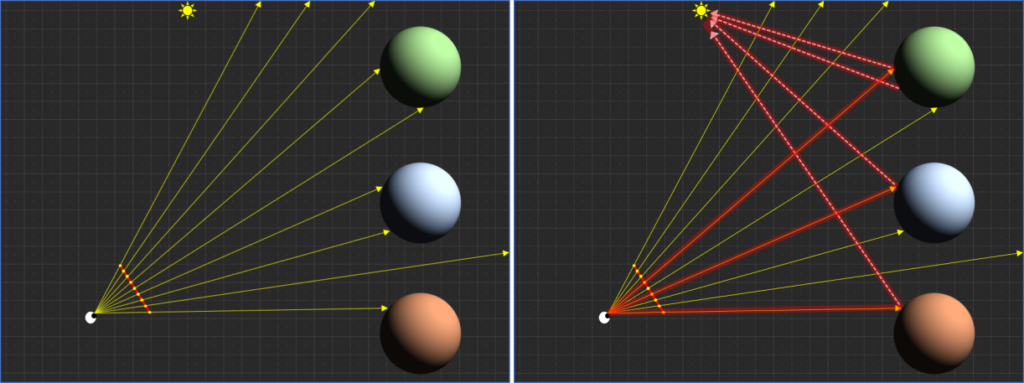
1. Per-frame Sprite Data Traffic

As can be seen in Figure 6 and 8, most remedial sprites are small, often just a few pixels. It thus seems a waste to write full sprite pattern data each frame. Instead, DELTA keeps track of occupied lines in sprites. In subsequent frames, these lines are either overwritten with new data, or cleared.

A few examples: A sprite that stores two lines of data that becomes unused in the next frame will have these two lines cleared using two single-byte writes. A sprite that stores three lines while in the next frame that same sprite stores only two lines will have those two lines overwritten (for patterns and colours), and the third line cleared (just the pattern).

At the expensive of some non-trivial administration, this approach greatly reduces bandwidth for sprite patterns. A further reduction is possible if we do not overwrite colour data if this did not change, but it turns out that this is too rare to justify the cost of checking this.

Table 1 shows the sprite traffic of several frames of track 1.

Frame##SpritesAvg lines10131.5420112.003075.4340123.7550113.45

2. Compressing Tile Colours

As can be seen in Figure 5, tiles for a particular frame often use only two colours. We thus split all tiles in two groups: One group for 2-colour tiles, and one group for tiles that require more colours. The 2-colour tiles are then sorted in such a way that large continues spans of the same colour values emerge. Figure 5 clearly shows this. Run-length encoding of this data becomes very effective, reducing tile colour data to a fraction of its original size.

The run-length scheme used in DELTA is simple and translates to efficient Z80 assembler for decoding directly to VRAM. The compressor distinguishes two types of span:

1. ‘Uniform spans’, storing three or more identical values, with a maximum length of 128 pixels
2. ‘Raw spans’, storing arbitrary values, also with a maximum length of 128 pixels.

A span starts with a single byte that stores the span type in 1 bit and the length in the remaining 7 bits. To speed up decompression, a raw span is assumed to be followed by a uniform span.

The core of the Z80 decompression code is shown below. Timings include the M1 wait on MSX, as specified on Grauw’s website.

      ...  setup VRAM access
      ld a, (hl)          // 7  - get first command
loop:						
      rra                 // 5T  - lowest bit contains span type (1)
      ld b, a             // 5T  - b = length of raw span
      jp c, dospan        // 11T - span is uniform?
      inc hl              // 7T  - advance input stream pointer
      otir                // 23T - emit 'b' bytes reading from [hl]
      ld b, (hl)          // 7T  - b = length of uniform span minus two
dospan:
      inc hl              // 7T  - advance input stream pointer
      ld a, (hl)          // 7T  - a = value for uniform span
      out (0x98), a       // 12T - write first pixel of span (2)
      inc hl              // 7T  - advance input stream pointer
      out (0x98), a       // 12T - write second pixel of span (2)
      nop                 // 5T  - VDP timing (3)
uniform_loop:
      out (0x98), a       // 12T - write remaining span pixels
      djnz uniform_loop   // 14T - while (--b) goto uniform_loop
      xor (hl)            // 8T  - obtain next command (4)
      jp nz loop          // 11T - if not zero: next pair of spans (5)

The run-length decompression code is pivotal for the performance of the renderer. It has thus been very carefully crafted. Some details:

1. The span type is stored in the lowest bit of each span header. This way, it can be shifted into the carry flag using the rra instruction.
2. A uniform span is at least three pixels. The first two are drawn unconditionally, outside the loop.
3. The nop is needed to avoid timing issues for the VDP, as the out instruction before it takes less than 15 cycles.
4. After the first two spans, span headers are xor’ed with the value used in the previous uniform span. This way, a single xor (hl) sets the zero flag on end-of-stream while obtaining the next command in all other cases.
5. The final span must be a uniform span (of at least three bytes), even if the input data does not need this. For this reason, the target buffer must have room for this dummy span. In DELTA, line 23 in the name table starts with three spaces for this reason.

And finally: Instead of the final jp nz it is more efficient to unroll the code (several times), as not taking a jump is faster on the Z80. DELTA unrolls the code three times for this purpose.

Frame#Colour data sizeCompressed sizeRatio10156819612.5%2015921368.5%3017321669.6%4015761408.9%50166420412.3%

Table 2 shows details on the compression of tile colour data. Simple run-length encoding is able to decimate the data rate here.

3. Compressing Tile Patterns

At first sight, tile pattern data appears to be mostly random and thus unsuitable for basic run-length encoding. It turns out however that this is worthwhile.

DELTA further improves run-length encoding of tile pattern data using random reordering. This is based on the observation that the order of tiles within a slice of equally coloured tiles is irrelevant; swapping two tiles (along with their indices in the name table) yields the same image. We obtain a near-optimal ordering using a random process, in which we repeatedly swap tiles and assess the rate of compression, keeping advantageous mutations.

Table 3 shows the result of tile pattern compression. Although compression is not nearly as efficient as in the case of colour data, size is still almost halved in many cases.

Frame#Pattern data sizeCompressedCompressed (mutated)Ratio101568105095861.1%201592112899662.6%301704107992754.4%401576100985354.1%50166495580548.4%

4. Compressing the Name Table

Each frame uses 32×23 tile indices in the name table (the last line of tiles displays score and such). Like the tile colours, this data is run-length compressible, although the gains are often modest.

We found that for some complex frames maintaining 20fps was difficult. Therefore, name table compression is made optional: It is skipped when the tile count exceeds a certain threshold, which is a good indicator for frame complexity. Copying raw data is always faster than decompression; by making it adaptive we sacrifice compression efficiency for rendering performance. If needed, this could be extended to other data, e.g. the tile pattern data.

Table 4 shows the efficiency of name table compression. Compared to colour and pattern data, name table compression shows somewhat poor compression.

Frame#Compressed sizeRatio1042958.3%2045461.7%3047063.9%4046563.2%5046963.7%

5. Storing Frames in Segments

After compressing all data for a frame, the end result is somewhere between 800 bytes and 2 kilobytes, with an average size of 1695 bytes for track 1 frames. This data has to be stored in one of the 16KB segments of the final megarom, and for efficiency reasons, it should not span a segment boundary. At 1695 bytes per frame, this would leave (on average) a gap of 848 bytes at the end of each segment, which is a 5% waste of space.

Here we again use the stochastic optimization approach. After generating all track frames, we reorder them in such a way that each megarom segment is as full as possible. For the 802 frames of track 1, this reduces wasted space in the segments to just a few bytes.

Future Work

As stated in the previous paragraph, compression of track data yields an average size of 1695 bytes per frame, which is a solid improvement over storing raw data, while still allowing run-time decompression. There is however room for improvement.

To improve rendering speed and compression efficiency, we should reuse data more often. The tile colour table is 2KB for 256 characters; yet from frame to frame tile colours will be similar. We may be able to avoid writing a substantial part of that 2KB if we carefully order our tiles. This would however require a strict sequential decompression of frames, potentially using occasional keyframes.

Similarly, we could simply leave all (or most) tile colours untouched, by predefining groups of tiles with specific colour pairs.

If memory capacity increases even further, it may be advantageous eventually to discard compression altogether. Clever reuse of frame-to-frame coherence then becomes the only useful scheme.

And finally, we did not explore the use of a dynamic palette. Currently a track can use 16 colours, of which 3 are shared with the player car and another one (white) with the score display. The remaining 12 colours are rarely in view at the same time, which should allow for more freedom in this regard.

Concluding Remarks

The main technical contribution in DELTA is, we believe, the use of GRAPHIC4 mode combined with sprites to display pre-rendered polygon graphics. The available bandwidth and sprite count allows for a level of detail that is sufficient for a 256×192 display, as evidenced by the game.

Additionally we demonstrated that basic run-length encoding is effective for all data streams: Although tile colour data benefits most, tile pattern data and name table data still benefit substantially, while decompression remains simple enough to be used at 20fps on the Z80 CPU.

Finally, we indicated several avenues for further improving the technique. This could either allow for higher frame rates (25 fps seems feasible), more complex scenery, a larger display (using ‘overscan’ for 26.5 lines of tiles), or more complex game play and/or music.

The technique does impose strong limitations on gameplay. When properly mitigated, we believe the proposed technique provides a visual style that is rather unique for the platform.

Playing DELTA

DELTA has been submitted to the MSXDev25 competition and can be played for free via File-Hunter.com.

Contact us in case of questions / remarks: bikker.j@gmail.com.

Abstract

This article describes some recent experiments in the quest for the “Ultimate BVH” for ray tracing in games. We revisit several algorithms: full sweep SAH BVH construction, binned construction, H-PLOC for GPU, spatial splits, and BVH optimization by reinserting subtrees. We show that spatial splits have a major impact on BVH quality for typical ‘game-like’ scenes. Additionally, the bin count that is used in BVH construction turns out to be important. And finally, we take some steps towards better BVHs by evaluating and optimizing BVHs using a Representative Ray Set.

BVH 101

A Bounding Volume Hierarchy (BVH) is a data structure that is used to quickly find the intersection between a ray and primitives (e.g. triangles) in a scene. For this article we will assume some familiarity with the basic concepts. Introductions to the topic can be found in the extensive survey by Meister et al., in Peter Shirley’s book, at Scrathapxiel, or in a series of blog posts on the topic.

An important tool to build high-quality BVHs is the Surface Area Heuristic (SAH). The SAH lets us pick a ‘good’ split plane position (and axis) during subdivision. Compared to naive splitting (e.g. half-way the longest axis or at the object median) the SAH yields trees that can be intersected in about half the number of traversal steps. It achieves this by selecting the split plane that minimizes intersection cost, which is estimated as the number of triangles on either side of the split plane, scaled by the probability that these triangles will have to be intersected by an arbitrary ray. This probability, in turn, is proportional to the surface area of the axis-aligned bounding box around the triangles.

We thus minimize:

C_{split}=N_{left}A_{left} + N_{right}A_{right}

Using the SAH has a downside: It must be evaluated at every point where N_left and N_right change, along each axis. A naive implementation has an algorithmic complexity of O(N^2) per split, which is prohibitively slow.

One way to alleviate this is by using binned building.

Here, instead of evaluating the cost function at every triangle, we evaluate it at N discrete intervals. Good results are obtained for N=8 or N=16.

Alternatively, the naive O(N^2) algorithm can be replaced by a more efficient version. By sorting the primitives along each axis and keeping them sorted during partition, a full sweep is achieved in linear time. This is still more expensive than binned building, but it does provide us with a baseline for SAH BVH quality, even for complex scenes.

Full-sweep, binned SAH and spatial split builders thus all use the SAH to steer split plane positioning. But, splitting is always greedy: The split plane is chosen as if the next split is the last one, without considering consequences for splits in subsequent levels of the tree. Therefore, even if the local decision is optimal, at a global scope this may not be the case.

At the global scope, we can use the surface area heuristic to assess overall tree quality. A good tree requires a ray to visit as few nodes as possible, while minimizing the chance that triangles must be intersected. Tree cost can be estimated as:

SAH=\sum_{node} Cost(node)\frac{Area(node)}{Area(root)}

This can be evaluated with a simple for-loop. In this formula, the relative area represents probability, while Cost(node) is the CPU/GPU effort for performing a traversal step or intersecting triangles.

Assumptions

So far we have made several assumptions or followed common knowledge. E.g.:

1. Full-sweep SAH is ground truth. Binning is an approximation. A full-sweep SAH BVH will thus always be better than a BVH built with binning.
2. Bin counts matter. More is better. N=4 yields reasonable trees; N=8 is a good trade-off of quality and build speed; N=32 shows diminishing returns.
3. ‘Better’ in the previous assumption means: ‘Yields lower SAH’. And: ‘Lower SAH means more fps’.

It turns out that all of these assumptions are incorrect, at least to some degree.

SBVH

Before we go into more detail, two advanced tools for improving BVH quality must be discussed: Spatial Splits, as proposed by Stich et al. in their 2009 HPG paper, and insertion-based optimization, as proposed by Bittner et al. in a 2013 paper.

Spatial splits help when the optimal object split produces bounding boxes that significantly overlap. In such a case, splitting the triangles may alleviate the issue. This is illustrated in the above image. Note that in this example the split decreased surface areas, but increased triangle (or triangle reference) counts.

Spatial splits greatly help in scenes with a mix of small and large triangles. Consider the following situation:

Here, the presence of a large plane that intersects the teapot would prevent important horizontal splits in the bounding boxes.

For many scenes, a BVH built with spatial splits substantially improves upon a regular BVH. The gains are scene dependent, but a reduction of overall SAH cost of 25% or more is not uncommon.

Optimizing a BVH

The second tool is BVH optimization, which is applied as a post-process to an existing BVH. Several methods exist, but the current best one is reinsertion-based optimization. TinyBVH has an implementation for CPU, but a parallel version of the algorithm for GPU (by Meister and Bittner) also exists.

The concept is simple: We take a random node from the BVH, remove it (along with the subtree attached to it), and reinsert it elsewhere. The result is a valid BVH, which often has a different overall SAH cost. If this cost is lower than before the change, we keep the change, otherwise we revert it.

The process can be improved by carefully selecting the nodes to be reinserted and by carefully selecting the new position in the tree. See the paper for full details.

The parallel version of the algorithm is important for GPU BVH construction. Efficient GPU BVH construction is often based on the LBVH algorithm, which is very fast, but yields low-quality BVHs. However, applying the parallel reinsertion (‘PRBVH’) algorithm magically turns the bad BVH in a good one.

More Assumptions

Let’s formulate some more assumptions, related to SBVHs and optimization.

1. We can optimize a bad BVH into a good BVH.
2. So, we can optimize an SBVH into the ultimate BVH.
3. Optimizing will never make things worse.

To start with the first assumption: For GPU BVH builders, this is true. Later papers often use the quality of PRBVH as a baseline. See for example the recent H-PLOC algorithm, which sacrifices about 8% SAH cost to improve BVH construction speed.

One thing reinsertions cannot do is triangle splitting. Once a BVH has been built without splits, large leaf nodes keep their surface area; no node shuffling can resolve that.

Reinsertions can however be used to optimize an SBVH. Unlike e.g. refitting, reinsertions operate only on node bounds – the original triangle data is never accessed. But, results are confusing. Often an optimized SBVH will have a lower SAH cost, but actual ray tracing performance lags behind – or even deteriorates.

Regarding the final assumption: This is not something the original paper claims. In the tail of the process SAH cost starts fluctuating:

A more recent paper by Meister and Bittner addresses this issue using simulated annealing to get out of potential local minima.

Setup Camp

Let’s interrupt the quest for the Ultimate BVH for a moment to assess the situation.

A good BVH is constructed using the Surface Area Heuristic and Spatial Splits. Optimizations can approximate SBVH quality without splits, but intuitively, optimizations should not replace splits: Both techniques should be used together.

SBVH construction requires binning. We can use a full-sweep for object splits, but finding the optimal spatial splits is only practical using bining.

For an optimized SBVH, SAH appears to behave erratically. Specifically, it is unclear if the assumed relation between SAH cost and ray tracing performance holds.

We have questions.

1. What is the optimal bin count for an SBVH?
2. Is there a better heuristic than SAH?
3. Can we combine spatial splits and optimization by reinsertion?

And, perhaps one underlying question, related to the main quest:

1. Compared to the BVHs used for hardware ray tracing, how much better can be do if build cost is not an issue?

We continue.

Representative Ray Set

Although the Surface Area Heuristic is generally assumed to be useful in BVH quality assessment, it has its limitations. A paper by Aila et al. titled “On Quality Metrics of Bounding Volume Hierarchies” addresses the issue and proposes a more accurate metric, called End Point Overlap (EPO). More metrics exist; a good overview is provided in the master’s thesis by Athos van Kralingen.

All metrics ultimately aim to estimate ray tracing cost of a BVH. We could simply measure this cost directly, but this is non-trivial: Varying architectures, operating system overhead and unstable processor speeds all add noise to direct measurements. What we can measure however is the average traversal step count and triangle intersection count for a Representative Ray Set (RRS), which was proposed in a paper by Bittner and Havran.

For interior scenes we construct such a set as follows. An 8x8x8 grid of path spawners is placed in the scene. From these locations we start paths in a random directions, bouncing up to 10 times. We select path segments from these paths and place them in four buckets:

1. Primary rays, which start in empty space and end on a surface in the scene.
2. Short secondary rays, which start and end on a scene surface and have a length of at most 5% of the largest scene dimension.
3. Long secondary rays, which also start and end in the scene but have a greater length.
4. Sky rays, which start on a surface and then leave the scene.

For exterior scenes and objects we want to prevent generating spawners inside the object, so we instead place the spawnes on a sphere surrounding the scene.

The size of the set is chosen based on scene detail. For most scenes 1 or 2 million rays in the set give good results.

Bin Count

We first test the RRS on the effect of bin count on the quality of a BVH. For our experiments we use the following six scenes:

The Sponza Atrium scene (Crytek version) is a moderately complex scene with large and small triangles. Many triangles are axis-aligned. The Lumberyard Bistro scene (exterior only) is a larger scene, with more freely oriented objects and buildings. The Conference Room is a well-known test scene for BVH construction. The Lego Car is a simple hand-crafted model with smaller and larger triangles. The Stanford Dragon has lots of triangles of mostly uniform size. The San Miguel scene finally is included because of its size (about 10M triangles).

We started with the assumption that binned builds yield inferior quality to a full-sweep build and that more bins is better. That turns out to be incorrect:

In fact, the lowest SAH cost that was found for this scene is 37.99, while 44 bins yielded an SAH cost of 41.04, an 8% difference. Other scenes show similar behavior: 8% is not an outlier.

If we use the new Representative Ray Set, the graph changes somewhat:

Using the RRS metric, bin count still has no relation to BVH quality. And, although the results are similar to SAH figures, there are also differences: E.g., RRS indicates that 8 and 10 bins should yield similar performance, while SAH expects a significant difference.

It turns out that finding the optimal bin count for each scene yields a substantial improvement over default SBVH quality, regardless of which bin count is chosen by default. TinyBVH by default uses 8 bins for SBVH builds. We searched for the optimal bin count between 8 and 128 bins for the six scenes, and included ‘half bin counts’, where odd levels in the BVH use one extra bin. The results are shown below.

SceneRRSRelative to 8 binsSponza27.5+1.64%Conference31.5+9.63%Dragon123+4.98%Bistro105+8.76%Lego Car56.5+5.67%San Miguel27+5.58%

The percentage shown here is the ray tracing performance improvement estimated by the RRS metric. All scenes benefit from selecting an optimal bin count, but the Conference Room and Bistro improve most.

Optimizing using the RRS

Starting from a high-quality SBVH we can now attempt to optimize further using reinsertions. We apply the following procedure:

1. A copy of the BVH is made to be able to restore it later.
2. The BVH is optimized by reinserting a subset of the nodes.
3. The resulting BVH quality is assessed using the RRS metric.
4. If the quality of the tree did not improve, the pass is undone.

Applying this process to the Sponza Atrium Scene we obtain the following data:

Sponza AtriumSAHRRSrel SAHrel RRSFull-sweep84.2934.11referencereferenceBinned SAH, 8 bins80.5430.95+4.66%+10.22%Optimized binned73.6228.36+14.50%+20.31%SBVH, 8 bins73.7323.36+14.31%+46.02%SBVH, 32 bins73.5124.00+14.67%+42.19%Optimized SBVH, 32 bins70.1823.05+20.10%+47.99%SBVH, best bin count71.2322.87+18.33%+49.14%SBVH, final65.0220.82+29.63%+63.82%

There is a lot of information here. The baseline is the full-sweep SAH builder, which, for this scene, yields an SAH cost of 84.29 and an RRS cost of 34.11.

A binned SAH BVH, built using 8 bins, surprisingly does better than full sweep. This BVH can be optimized too, and the result is better than optimizing the sweeped BVH. This indicates that the input quality for the optimizer does matter.

When we switch to SBVH, RRS and SAH start to disagree. For an SBVH built with 8 bins, SAH expects a tree quality similar to ‘optimized binned’ (+14%), whereas RRS expects an improvement over baseline of no less than 46%.

The best BVHs for this scene are obtained with the optimal bin count and using the RRS-steered optimization process. The final BVH is expected to perform 30% better according to SAH, and almost 64% better according to RRS.

Timing RRS

The discrepancy between SAH and RRS begs the question: Which one is right? To answer this question we measured ray tracing performance on CPU and GPU. The table below shows the results for the Bistro scene.

Bistrorel SAHrel RRSrel CPUrel GPUFull sweepreferencereferencereferencereferenceH-PLOC-5.35%-4.28%-0.44%-9.44%Binned (8)-17.72%-11.06%-6.13%-21.66%SBVH (8)+43.45%+66.78%+48.88%+77.71%SBVH (best)+49.96%+81.21%+61.66%+87.80%SBVH (ours)+63.08%+99.10%+65.63%+89.99%

The measurements for this table are conducted on a Ryzen 9 CPU and 780M GPU. TinyBVH 1.5.4 is used to trace (individual) rays; the BVH layout used here is the BVH8_CPU layout. The H-PLOC BVH is constructed using the open source NexusBVH tool and postprocessed to combine leaf nodes. For GPU ray traversal the 2-wide BVH_GPU layout of TinyBVH is used.

The timings reveal something interesting: First of all, RRS appears to over-estimate the quality of the BVH. But also: SAH is a good metric for CPU performance, while RRS seems to predict GPU performance better.

Note that for this scene spatial splits greatly affect overall performance. Not using this optimization is costly: While – compared to the baseline full-sweep algorithm – 78% more rays can be traced with an SBVH, the difference between H-PLOC and SBVH is greater. Beyond the 8-bin SBVH, picking an optimal bin count helps further, while the effect of the (costly) RRS optimization scheme is limited for this scene.

Finally, here are some results for the remaining scenes.

Stanford Dragonrel CPUrel GPUH-PLOC-14.39%-16.28%Binned (8)-4.26%+0.41%SBVH (8)-3.74%+0.33%SBVH (best)-0.13%+4.57%SBVH (ours)-1.02%+8.06%

For the Stanford Dragon scene the baseline full-sweep SAH builder is hard to beat. Spatial splits have little impact. Picking the best bin count remains important however: The predicted 5% gains mostly materialize, but only on the GPU. The CPU does not even benefit from the RRS optimization process. On the GPU, this yields a Dragon BVH that is 8% faster than the full-sweep BVH, and considerably faster than H-PLOC.

Lego Carrel CPUrel GPUH-PLOC-0.86%+6.97%Binned (8)+3.66%+8.50%SBVH (8)+6.87%+22.55%SBVH (best)+17.04%+18.88%SBVH (ours)+15.62%+20.84%

Unlike the Dragon, the Lego Car model does have a mix of large and small triangles, which justifies the use of spatial splits here.

San Miguelrel CPUrel GPUH-PLOC-5.89%-15.04%Binned (8)-4.63%-12.36%SBVH (8)+3.55%+11.10%SBVH (best)+14.18%+14.06%SBVH (ours)+16.52%+17.69%

San Miguel does not provide any new insights. The scene benefits somewhat from spatial splits, but most of the geometry consists of small details, limiting the impact.

Further Details

The full data set produced for these experiments is available here. The experiments can be replicated using the code on the TinyBVH repository on Github using the tiny_bvh_optimizer project.

Concluding Remarks

By carefully combining existing techniques and observing the effects of factors like bin count it is possible to improve beyond the quality of an SBVH. For some scenes performance is doubled compared to H-PLOC and the baseline full-sweep algorithm. It seems attractive to reconsider the option of offline BVH construction for static geometry, which is an option that is currenly often ignored for ray tracing in games.

For future work we would like to further investigate the option of software ray tracing on GPUs. Gaining insight in the actual advantage of ray tracing hardware and opening up this hardware for new construction and traversal algorithms is crucial for making progress. Making high-quality BVH tools available as open source software contributes towards this goal.

So, as a popular game repeatedly reminds us: We continue.

Acknowledgements

This research was supported by AMD who kindly provided the test machine.

References

A Survey on Bounding Volume Hierarchies for Ray Tracing, Meister et al., Eurographics 2021.
Assessing Alternatives to the Surface Area Heuristic for Bounding Volume Hierarchy Construction. Van Kralingen, Master’s Thesis, Utrecht University, 2023.
Automatic Creation of Object Hierarchies for Ray Tracing, Goldsmith & Salmon, 1987.
Fast BVH Construction on GPUs, Lauterbach et al., Eurographics 2009.
Heuristics for Ray Tracing Using Space Subdivision, MacDonald & Booth, 1990.
H-PLOC: Hierarchical Parallel Locally-Ordered Clustering for Bounding Volume Hierarchy Construction, Benthin et al., 2024.
On fast Construction of SAH-based Bounding Volume Hierarchies, Wald, 2007.
On Quality Metrics of Bounding Volume Hierarchies. Aila et al., High Performance Graphics 2013.
Parallel Reinsertion for Bounding Volume Hierarchy Optimization, Meister & Bittner, 2018.
Performance Comparison of Bounding Volume Hierarchies for GPU Ray Tracing, Meister & Bittner, 2022.
RDH: Ray Distribution Heuristics for Construction of Spatial Data, Bittner & Havran, 2009.
Spatial Splits in Bounding Volume Hierarchies, Stich et al., 2009.

Further Reading / Contact

Want to know more about BVHs? There is a series of 10 posts about it on my blog:

1. Basics: data structure, simple construction and ray traversal

Alternatively, you can read about advanced ray tracing techniques using voxels:

1. Ray Tracing with Voxels in C++ Series – Part 1

Other topics on the blog include probability theory, software optimization and retro game development.

I can be found on BlueSky, LinkedIn and ProtonMail.

Thanks for reading!

This document describes the tinybvh single-header library for Bounding Volume Hierarchy construction and traversal, with a focus on ray tracing – to be used for graphics, audio or physics.

This document is currently in sync with tinybvh version 1.3.3. It will be frequently updated.

Tinybvh is open source (MIT license) and available on Github.

The manual is split up in multiple compact documents:

1. Basic Use. Building a BVH, tracing a ray, alternative layouts, TLAS/BLAS.
2. Advanced Topics (this document). GPU ray tracing, custom math libraries, tinybvh settings.

Introduction

The first part of the tinybvh manual discussed basic use of the single-header library. In this second part presents several more advanced topics. An overview:

• Using indexed triangles and vertex buffers
• Building BVHs for the GPU: Layouts, considerations and best practices
• Replacing the tinybvh math library
• Double-precision BVHs
• BVH optimization
• Memory management: Design, callbacks
• Using custom geometry
• Collision queries
• Low-level settings

Data Ownership, Indexed Input, Slices

The standard input for all builders is a raw list of four-component vectors. These are used in two places:

• During BVH construction: Each triangle is turned into a fragment, which stores AABB of the triangle and the index of the original.
• During traversal: To intersect a triangle in a BVH leaf node, the original triangle data is needed.

The triangle data that is passed to BVH::Build / BVH::BuildHQ / BVH::BuildAVX is thus kept and should not be destroyed or changed between BVH construction and BVH traversal. Ownership of the data does however stay with the calling application.

In some cases it is inconvenient to pass data in this exact format. For example when tinybvh should operate on data that is also used by a rasterizer, where the vertex stream may contain x, y, z but also u, v and perhaps normal data. For this purpose a bvhvec4slice can be used (tiny_bvh.h, line 287). This struct encapsulates the vertex data pointer, along with a stride (in bytes). For four-component vector input, the stride defaults to 16.

Using a bvhvec4slice as input for the builders has no impact on performance – In fact, passing a raw bvhvec4 pointer results in the creation of a slice with stride 16. Do note however that BuildAVX requires each vertex to start at a 16-byte boundary in memory. If this can not be enforced, please use Build or BuildHQ.

Apart from vertex buffers, rasterizers also typically use vertex indices to define each triangle. To support this input, each Build function accepts (next to the vertex list) an index list. An example:

bvh.Build( (bvhvec4*)verts, (uint32_t*)indices, TRIANGLE_COUNT );

If indices are provided, they will be kept along with the vertex data for use in the traversal functions. Please be aware that this adds a level of indirection when accessing vertex positions in the triangle intersection code; indexed data is therefore slower than a raw list of bvhvec4‘s.

GPU BVHs

Tracing rays on the GPU is these days typically done with dedicated hardware. This hardware reduces the computational cost of BVH traversal and triangle intersection – it does however not magically increase the memory bandwidth of the GPU. It is therefore most effective when bandwidth is not the bottleneck.

In a typical ray tracer this is the case for coherent primary rays (those leaving the camera) and shadow rays. Rays after a bounce are more divergent and tend to be more expensive. These rays also require more bandwidth, which somewhat limits the possible gains of the dedicated ray tracing hardware. Especially for these scattered rays the quality of the BVH is important. All vendors thus provide their own BVH builders, which generate BVHs that are hardware-specific and finely tuned.

Tinybvh will currently not create BVHs in these vendor-specific formats – although this may be different in a later version of the library, at least for vendors that disclose their BVH formats (currently: Intel, and to some extent, AMD).

Instead, tinybvh will produce several layouts that work well for GPUs in general. As on CPU, there is a balance to be found between BVH construction time and ray traversal time. Currently three GPU BVH layouts are available:

• BVH_GPU: This layout follows the recommendations in a 2009 paper by Aila & Laine. This BVH layout is quickly obtained from the default BVH layout and offers reasonable ray tracing performance. The traversal kernel is short and simple and can easily be implemented in any shader or GPGPU language.
• BVH4_GPU: This layout uses a wide (and thus shallow) BVH to speedup traversal of divergent rays. The reduced number of traversal steps improves memory coherency at the expense of more calculations per step, which is a good trade-off in most cases. Conversion is however more expensive than for the BVH_GPU layout.
• CWBVH: This is the final layout proposed by NVIDIA before introducing their RTX hardware. CWBVH uses an 8-wide BVH with heavily compressed nodes. Additionally, triangle data is stored without any indirection interleaved with the nodes for optimal access. This is a fast layout, but obtaining it is relatively costly. This is mostly useful for static geometry. Also note that the traversal kernel is complex; it requires specialized bit manipulation instructions to run at full speed. Porting this code will be challenging.

Note that all vendors construct their BVHs on the GPU, rather than on the CPU. Tinybvh on the other hand assumes that BVHs are constructed and maintained on the CPU. This is because CPU builders tend to build better BVHs, and, more importantly: Because CPUs are typically under-utilized in modern games. Even if the CPU requires more time to prepare the BVH, frame time improves if we move the task from the GPU to the CPU so that building and tracing are done in parallel rather than sequentially on the faster processor. NB: Several of these claims require experimental validation.

Bring Your Own Math Library

Vector math inside tinybvh is handled by a small set of structs, and a minimal set of operators. These can be found in tiny_bvh.h, starting on line 243:

• bvhvevc2/3/4
• bvhint2/3
• bvhuint2
• bvhaabb
• bvhdbl3

These structs only exist to avoid dependency on an external math library. Applications using tinybvh probably already use their own math classes, e.g. Eigen or glm. The included structs (with uncommon names) aim to avoid collisions.

Additionally, it is possible to use your preferred math library. For this, simply define TINYBVH_USE_CUSTOM_VECTOR_TYPES before including tiny_bvh.h, and inform tinybvh about your types, e.g.:

namespace tinybvh
{
   using bvhint2 = math::int2;
   using bvhint3 = math::int3;
   using bvhuint2 = math::uint2;
   using bvhvec2 = math::float2;
   using bvhvec3 = math::float3;
   using bvhvec4 = math::float4;
   using bvhdbl3 = math::double3;
}

From here on, tinybvh will now use your math library. Two notes:

1. The float3 / bvhvec3 type must be 12 bytes in size.
2. The unconventional double vector type is not needed if double precision functionality is disabled (see the section on double precision and/or settings).

Double Precision

In some exceptional situations a scene may require double precision numbers. For this, tinybvh offers a double precision BVH layout, in which every floating point number is stored (and processed) as a 64-bit value, greatly extending the range and precision.

A double precision BVH is constructed like a regular one:

BVH_Double bvh;
bvh.Build( (bvhdbl3)triangles, TRIANGLE_COUNT );

Note that the input triangles are specified here with three doubles – not four; the BVH will not be constructed with AVX code and does not have the data alignment restriction of the regular BVH.

A double-precision BVH is intersected with a double-precision ray. The struct for this is tinybvh::RayEx:

RayEx ray( O, D );
bvh.Intersect( ray );

The ray origin and direction in RayEx are specified as double precision values.

To build a TLAS over double-precision BVHs, use the InstanceEx struct. Other than this, TLAS construction is the same as with regular BVHs. And, like regular BVHs, a double-precision BVH can be constructed over custom primitives.

The double-precision functionality is demonstrated in the tiny_bvh_anim_double.cpp example.

Optimizing a BVH

Once a BVH has been built, it is possible to optimize it. This can have significant effect on performance: It is possible to improve ray tracing speed by about 20% this way.

Tinybvh implements an algorithm described in a 2013 paper by Bittner et al., which reorganizes BVH nodes to decrease overall SAH cost. The implementation of the paper is a partial one; as a consequence optimizing a BVH is quite time consuming. This will be improved in a future version of tinybvh.

To experiment with it now, use the following process:

BVH_Verbose* verbose = new BVH_Verbose();
verbose->ConvertFrom( *bvh );
verbose->Optimize( 1500000 );
bvh->ConvertFrom( *verbose );

This flow uses the special-purpose BVH_Verbose layout, which is required for the optimizer. The optimizer than makes a large number of attempts to move nodes to a better location in the BVH. Depending on the overall size of the BVH, diminishing returns are to be expected after 100k to 1M attempts.

After optimizing the BVH it must be converted back to the regular layout to be used in ray tracing.

Memory Management

The construction of a BVH requires several buffers:

• A fragment buffer, which contains the AABBs for the primitives
• A list of BVH nodes
• A list of primitive indices, used to efficiently sort primitives during conversion

Depending on the BVH layout, additional buffers may be needed.

Some applications may require that allocation and de-allocation is handled by a custom memory manager. This is supported by tinybvh via the BVHContext, which can be passed to the default constructors of all BVH layouts. By default, this struct contains two function pointers:

• One to malloc64, which allocates memory aligned to a cache line boundary,
• And free64, which frees memory allocated by malloc64.

Tinybvh exclusively uses these two function pointers to allocate and de-allocate memory. Override these function pointers to use your own functions.

Custom Geometry

The standard primitive type in tinybvh is the triangle. In cases where other primitives are required, these can be added as custom geometry. In this case, the application must implement three callback functions:

1. A function that calculates the AABB for a given primitive
2. A function that intersects a ray with a primitive
3. A function that detects a hit between a ray and a primitive.

A pointer to the first function must be supplied to BVH::Build() when the BVH is constructed. The other two must be set by overwriting the customIntersect and customIsOccluded fields of the bvh instance.

Note that a BVH can only support a single primitive type. To construct a scene of spheres and triangles for instance, one BVH should be constructed for the spheres, and one for the triangles. These can then be combined under a TLAS.

The custom geometry functionality is available both in regular BVHs and double-precision BVHs and is demonstrated in detail in tiny_bvh_custom.cpp and tiny_bvh_custom_double.cpp.

BVH versus Sphere

Although the BVH functionality of tinybvh focuses on ray tracing, a single physics-oriented operation is provided, which determines whether a BVH collides with a sphere:

bool hit = bvh.IntersectSphere( position, radius );

Here position is a three-component vector, and radius is a float. A double-precision version is currently not available, and the operation is currently only implemented for the default BVH layout.

It is worth noting that if you constructed a different layout, e.g. BVH_SoA, the underlying default BVH layout remains accessible, via the .bvh field of the alternative layout:

BVH_SoA soa;
soa.Build( triangles, TRIANGLE_COUNT );
bool hit = soa.bvh.IntersectSphere( position, radius );

Here, the efficient BVH_SoA is used for ray tracing, while the original BVH that the BVH_SoA was converted from is used for the sphere intersection.

Settings

Various defines are used in tinybvh to fine-tune desired functionality and performance. You can set these before including tiny_bvh.h in your application to override defaults.

• C_INT, C_TRAV : These values affect BVH construction. During construction the cost of intersecting a ray with a node is minimized using the SAH heuristic. This requires knowledge about the cost of traversing a node (C_TRAV) or intersecting a primitive (C_INT). Tweaking these values may improve ray tracing performance on a specific CPU or GPU or for primitives with custom intersection code.
• HQBVHBINS : Like the regular BVH builder, the SBVH builder uses a fixed set of discrete intervals to evaluate the ‘Surface Area Heuristic’ (SAH). A good tree is produced even with a modest number of intervals, but quality may improve somewhat with more intervals. The default is 8; values of 16 or even 32 may yield a (small) improvement of BVH quality, although this will significantly increase build time.
• INST_IDX_BITS : This value defaults to 32, which forces tinybvh to use a full 32-bit value to store the instance index of an intersection of a ray with a TLAS. Reducing this value to e.g. 10 allows tinybvh to combine the instance index with the primitive index, reducing the intersection data to 16 bytes. This is faster, but 10 bits means that only 1024 instances can be used, while the remaining 22 bits can index only 4 million triangles.
• NO_DOUBLE_PRECISION_SUPPORT : If defined, the double-precision BVH layout BVH_Double becomes unavaible, along with the double-precision vector type bvhdbl3. The main benefit of this is that a custom math library does not need to override bvhdbl3.
• NO_INDEXED_GEOMETRY : If defined, indexed vertices will not be available for BVH construction. This potentially slightly improves ray tracing performance, as the ray/triangle code otherwise must use an if-statement to determine the presence of indices. This effect should be limited for scenes that exclusively use either indexed or non-indexed geometry.
• NO_CUSTOM_GEOMETRY : If defined, custom primitive intersection via callbacks is disabled. Like NO_INDEXED_GEOMETRY this reduces or eliminates conditional code during intersection.
• TINYBVH_USE_CUSTOM_VECTOR_TYPES : If this is defined, tinybvh will not use its own vector types; instead it will assume you define these. See the relevant section earlier in this document.
• TINYBVH_NO_SIMD : Tinybvh will use SIMD via AVX or NEON on CPUs that support this. If you prefer the library without SIMD support, you can use this define.

And Finally…

This concludes the ‘Advanced’ section of the tinybvh manual.

Questions? Comments? Mail me at bikker.j@gmail.com or follow me on blueksy: @jbikker.bsky.social.

Manual index:

1. Basic Use. Building a BVH, tracing a ray, alternative layouts, TLAS/BLAS.
2. Advanced Topics (this document). GPU ray tracing, custom math libraries, tinybvh settings.

This document describes the TinyBVH single-header library for Bounding Volume Hierarchy construction and traversal, with a focus on ray tracing – to be used for graphics, audio or physics.

This document is currently in sync with TinyBVH version 1.6.2. It will be frequently updated.

TinyBVH is open source (MIT license) and available on Github.

The manual is split up in multiple compact documents:

1. Basic Use (this document). Building a BVH, tracing a ray, alternative layouts, TLAS/BLAS.
2. Advanced Topics. GPU ray tracing, custom math libraries, tinybvh settings.

Introduction

High-quality acceleration structure construction is non-trivial. A good BVH lets you trace hundreds of millions of rays per second on a modest CPU and even billions per second on a high-end GPU. It does this by hierarchically subdividing the scene. A ray can efficiently cull large groups of primitives if it does not hit the bounding volume of those primitives.

This is also the core functionality of NVIDIA’s RTX, Microsoft’s DXR and Intel and AMD’s ray tracing hardware. On the CPU, similar functionality is available in the form of Intel’s Embree.

So, TinyBVH arrives in a crowded place, but it does bring some specific characteristics and ambitions.

• For GPU, it aims to offer competitive ray tracing performance outside Vulkan, DirectX and CUDA. TinyBVH comes with short OpenCL traversal kernels (as well as OpenGL compute kernels) that can be easily ported to any API. This is already enabling fast ray tracing in WebGL.
• For CPU, it aims to offer a more accessible and compact framework than the awesome but complex Embree library.
• TinyBVH is a single-header library written in ‘sane C++’ and it comes with no dependencies. That means that adding tinybvh is incredibly simple: just include tiny_bvh.h.
• TinyBVH is fast. Both construction and traversal is at least competitive. The goal is to achieve state-of-the-art performance. Version 1.6.3 is very close to this on CPU and GPU.

This manual describes basic use of TinyBVH. It frequently points to the example code included with TinyBVH, which can be compiled on Windows, Linux and MacOS.

Basic Use

A basic example using the library can be found in tiny_bvh_minimal.cpp. The library is added to the file with an include:

#define TINYBVH_IMPLEMENTATION
#include "tiny_bvh.h"

The define before the include tells TinyBVH that this file needs the interface as well as the implementation. Other files can also include tiny_bvh.h, but only one C/C++ file should use the TINYBVH_IMPLEMENTATION define.

Now we can simply instantiate an empty bvh:

tinybvh::BVH bvh;

Next, we feed it some triangles:

bvh.Build( triangles, TRIANGLE_COUNT );

Here, ‘triangles’ is a list of vertices: three for each triangle. Each vertex is specified as a 16-byte ‘float4’ value, of which only 12 bytes are used for x, y and z. The reason for this ‘waste’ is performance: Internally, tinybvh will be able to operate much faster on 16-byte vertices.

With the BVH constructed, we can use it to fire rays:

tinybvh::Ray ray( O, D );
bvh.Intersect( ray );

The result of this operation can be found in ray.hit. This has a couple of fields:

• ray.hit.t: This is the intersection distance. If the ray hit nothing, this will be 1e30f (very far away). You can turn the intersection distance into an intersection location with the formula P = ray.O + ray.hit.t * ray.D.
• ray.hit.prim: This is the index of the triangle that was hit. You can find the vertices of this triangle in the array that was passed to bvh.Build. Note that ownership of this array remains yours; tinybvh just borrowed it for the construction and traversal of the BVH.
• ray hit.u and ray.hit.v: These are the ‘barycentric coordinates’ of the hitpoint on the triangle. These can be used to interpolate normals and textures.

Sometimes you don’t need all this information; perhaps you simply want to know if a ray can go from A to B unobstructed. This could be easily implemented with bvh.Intersect, but there is a better way:

tinybvh::Ray ray( O, D, 100 );
bool hit = bvh.IsOccluded( ray );

Note that the ray this time has a length: ‘hit’ will only be true if an obstacle is found between point O and a point along the ray, at a distance that is smaller than 100.

The distinction between the two ray queries is important, because a shadow ray is generally faster (about 30%) than the more generic ray query.

These are the basics. From here:

• Trace millions of rays. This is what TinyBVH is made for. You can also trace rays from multiple threads.
• Change the vertex positions and rebuild the BVH. Just call bvh.Build each time you change something.

That is probably all you need. The remainder of this manual discusses alternative BVH layouts with a different balance between construction speed and ray tracing speed, alternative geometry representations, using the BVH on the GPU and more.

Faster Construction

The BVH builder that is invoked with a call to bvh.Build is the reference builder. This is a multi-threaded binning SAH BVH builder, capable of processing ~200k triangles in 40ms, on a multi-core CPU. The reference builder code is fully cross-platform and has been confirmed to run on Windows, Linux, Mac (ARM) and the Raspberry Pi 4. You can find the source code in tiny_bvh.h, at the time of writing on line 2332.

To get better BVH construction performance, you can switch to the AVX-enabled builder. This one requires an Intel x64 compatible CPU. It cuts construction time (roughly) in half. To use it, simply write:

bvh.BuildAVX( triangles, TRIANGLE_COUNT );

In many cases this is the preferred option: The only drawback of BuildAVX is that it will not run on an ARM Mac or on the Raspberry Pi.

Faster Intersections

For static geometry it is often beneficial to sacrifice BVH construction performance to obtain a better BVH. Exactly what makes a better BVH is a complex topic (that article scratches the surface), but TinyBVH makes this easy. Just write:

bvh.BuildHQ( triangles, TRIANGLE_COUNT );

This invokes a state-of-the-art ‘spatial splits’ BVH builder to produce an SBVH. For 200k triangles, construction time will increase significantly to about 400ms, but after that, each ray will be about 25% faster. If you plan to use billions of rays for a path tracer, this may be a good trade-off.

Note that BuildHQ has several other drawbacks:

• It will use more memory. The performance improvement is achieved by cutting up certain triangles, which increases tree node count. A regular BVH will use about 32 bytes per triangle for the BVH (so: 6M for a BVH over 200k triangles); for an SBVH this is typically 15% more.
• Because of the unpredictable memory use, a BVH constructed with BuildHQ currently cannot be rebuilt. The SBVH builder really is intended for static geometry.

The availability of BVH::BuildAVX and BVH::BuildHQ allows you to optimize time to image (TTI), which is the sum of BVH construction and ray traversal time.

There are more ways to trace faster rays. We will discuss these next.

Alternative Layouts

In tiny_bvh.h you will find several alternative BVH layouts. One of them is BVH_SoA. To construct a BVH in this layout, simply instantiate and build it:

BVH_SoA bvh;
bvh.Build( triangles, TRIANGLE_COUNT );

Internally, this builds a regular BVH (tiny_bvh.h, line 4746), and converts it to a format that is easier to digest by an AVX-enabled CPU. This results in faster ray tracing performance: You can expect about 30% more rays per second when using BVH_SoA. And, it can be combined with BuildHQ: Just call BuildHQ on the BVH_SoA instance to combine the strengths of the SBVH with AVX ray traversal.

Some drawbacks to consider:

• Conversion is not an expensive step but it does take time. Do not use BVH_SoA if you have just a few rays to trace.
• The conversion does not destroy the original BVH. Effectively, you are now using twice the memory. It would not be impossible to change this (especially not for BVH_SoAs that you do not intend to rebuild) but for the moment, this is something to keep in mind.
• BVH_SoA traversal requires an AVX-capable processor (Intel x64 compatible), or an ARM NEON compatible processor (MacOS, Raspberry Pi). It is thus broadly supported, but not fully cross-platform.

A second CPU-centric layout is BVH4_CPU. It is constructed like other layouts:

BVH4_CPU bvh;
bvh.Build( triangles, TRIANGLE_COUNT );

Compared to BVH_SoA, this one is internally even more involved: To build a BVH4_CPU, tinybvh will first construct a regular BVH, which will be collapsed to a 4-wide bvh (layout BVH_MBVH<4>), which is finally converted to BVH4_CPU. This extra effort does result in a BVH that is very efficient.

BVH4_CPU requires an SSE4.2 capable CPU, which is at the time of writing pretty much every Intel-compatible CPU.

If your CPU supports AVX2, you can opt for the BVH8_CPU layout, which is even faster. This is the state-of-the-art BVH format, which comes within a few percent of the performance of Embree’s single ray queries.

Animation: Refitting

To trace rays in dynamic scenes, the most obvious option is to rebuild the BVH each frame. However, even for moderately complex scenes this does not allow for fluent frame rates.

Luckily, a full rebuild is rarely needed. We have two alternatives:

• Often a BVH can be refitted rather than rebuilt
• Often large parts of a scene do not require an update.

Regarding refitting: If the frames of an animated mesh are very similar, the BVH that we rebuilt each frame will also be similar. This is the case for example for trees that wave in the wind, or a water surface with some waves. In that case we can simply re-use a BVH and refit it around the changed geometry. This is a matter of updating bounding volumes, which is a lot more efficient than a full rebuild.

To refit a BVH, simply call the Refit method:

bvh.Refit();

This will use the triangle array pointer that you passed during construction. That means that the size of the list of triangles cannot change. Triangles should also not have changed position in the array; refitting really is only for smaller changes to vertex positions. When these conditions apply, refitting is very fast: A BVH for 200k triangles is refitted in less than a millisecond.

To exploit the fact that most geometry in a scene is static, we build not one BVH, but several. This is discussed in the next paragraph.

Animation: TLAS

Example program tiny_bvh_anim.cpp demonstrates the concept of the top level acceleration structure. In this example several BVHs are constructed:

• One for the static geometry of the Crytek Sponza scene (~262k triangles)
• One for a Stanford Bunny object.

Despite the name of the example there is no animation happening, but there is instancing: The bunny object is replicated in a 2x2x2 grid. For this an array of 9 instances is used, eight for the bunnies and one for Sponza:

BVH_SoA sponza;
BVH obj;
BVH tlas;
BVHBase* bvhList[] = { &sponza, &obj };
BLASInstance inst[INSTCOUNT + 1 /* one extra for sponza */];

For each instance a 4×4 matrix transform is set. After that the TLAS is constructed:

tlas.Build( inst, 1 + INSTCOUNT, bvhList, 2 );

We can now intersect the TLAS as if it were a regular BVH:

Ray ray( eye, D );
tlas.Intersect( ray );

The result is almost the same as intersecting a regular BVH. There is one difference: ray.hit.t this time also holds the instance index of the object that was hit. This is important, because triangle 1000 in Sponza is not the same as triangle 1000 in the bunny, and: Each individual bunny now has a model transform… This lets us intersect the same BVH multiple times, to paste the mesh in multiple locations (and if you wish, in multiple orientations).

The TLAS is a powerful tool. Take for example a racing game with 10M static triangles for the race track, plus 10 cars, each with a body mesh and 4 tire meshes:

• We calculate the BVH for the track once, at the highest possible quality.
• We calculate a BVH for the race car body and duplicate it 10 times, so we can change individual copies later.
• We calculate a BVH for a tire and replicate it 40 times, 4 times per car.
• To animate the cars, we change their transforms and rebuild the TLAS each frame.
• If a car gets damaged, we refit the changed model.

None of these operations involve a BVH rebuild, except for the TLAS. Constructing the TLAS for 51 objects will take far less than a millisecond. We now have a fully dynamic scene ready to be ray traced.

And Finally…

This concludes the ‘Basic Use’ section of the TinyBVH manual. See the index below for easy access to the Advanced Topics manual.

Questions? Comments? Mail me at bikker.j@gmail.com or follow me on blueksy: @jbikker.bsky.social.

Manual index:

1. Basic Use (this document). Building a BVH, tracing a ray, alternative layouts, TLAS/BLAS.
2. Advanced Topics. GPU ray tracing, custom math libraries, tinybvh settings.

In this series we build a physically based renderer for a dynamic voxel world. From ‘Whitted-style’ ray tracing with shadows, glass and mirrors, we go all the way to ‘unbiased path tracing’ – and beyond, exploring advanced topics such as reprojection, denoising and blue noise. The accompanying source code is available on Github and is written in easy-to-read ‘sane C++’.

This series consists of nine articles. Contents: (tentative until finalized)

1. Starting point: Voxel ray tracing template code. Lights and shadows.
2. Whitted-style: Reflections, recursion, glass.
3. Stochastic techniques: Anti-aliasing and soft shadows.
4. Noise reduction: Stratification and blue noise.
5. Converging under movement: Reprojection.
6. Path tracing: Basics first; then: Importance Sampling (this article).
7. Denoising fundamentals.
8. Acceleration structures: Extending the grid to a multi-level grid.
9. Acceleration structures: Adding a TLAS.

In This Article…

After all the noise and noise suppression techniques it is time to move forward and improve the visual fidelity of the renderer. We will do so using probably the most beautiful algorithm in computer graphics: Path Tracing. The core ‘ground truth’ algorithm turns out to be surprisingly simple – and stunningly close to the “God Algorithm”: Light transport (via photons) in the Real World.

At the end of this episode an extension to the basic path tracing implementation is introduced that improves its efficiency, while still producing an image identical to ‘ground truth’.

Starting Point

We start with a new scene: The “Floating Island of the Potion Brewer”, converted from a Sketchfab model by author Vilmariina. The scene is 256x256x256 voxels, so, in scene.h, set WORLDSIZE to 256. Then, load the scene using the following code:

Scene::Scene()
{
    grid = (uint*)MALLOC64( GRIDSIZE3 * sizeof( uint ) );
    gzFile f = gzopen( "assets/floating256.bin", "rb" );
    gzread( f, grid, sizeof( int3 ) );
    gzread( f, grid, GRIDSIZE3 * sizeof( uint ) );
    gzclose( f );
}

Next, replace Renderer::Trace (in renderer.cpp) by something simple:

float3 Renderer::Trace( Ray& ray, int, int, int depth )
{
    scene.FindNearest( ray );
    if (ray.voxel == 0) return float3( 1.2f, 1.2f, 1.0f );
    return ray.albedo;
}

That’s it, we’re all set.

Cheese

This time, we’re going to dive right in and start with the ‘finished product’. Run the code and find a camera view similar to the shot shown below.

Next, add the accumulator from Episode 3. Either go there for detailed instructions, or copy/paste the shortified code below, replacing Renderer::Init and Renderer::Tick:

void Renderer::Init()
{
    accumulator = new float3[SCRWIDTH * SCRHEIGHT];
    memset( accumulator, 0, SCRWIDTH * SCRHEIGHT * sizeof( float3 ) );
}

void Renderer::Tick( float deltaTime )
{
    static int spp = 1;
    const float scale = 1.0f / spp++;
#pragma omp parallel for schedule(dynamic)
    for (int y = 0; y < SCRHEIGHT; y++) for (int x = 0; x < SCRWIDTH; x++)
    {
        Ray r = camera.GetPrimaryRay( x + RandomFloat(), y + RandomFloat() );
        accumulator[x + y * SCRWIDTH] += Trace( r );
        float3 average = accumulator[x + y * SCRWIDTH] * scale;
        screen->pixels[x + y * SCRWIDTH] = RGBF32_to_RGB8( average );
    }
    if (!camera.HandleInput( deltaTime )) return; else spp = 1;
    memset( accumulator, 0, SCRWIDTH * SCRHEIGHT * sizeof( float3 ) );
}

And finally, replace Renderer::Trace by the following magical code snippet.

float3 Renderer::Trace( Ray& ray, int, int, int depth )
{
    scene.FindNearest( ray );
    if (ray.voxel == 0) return float3( 1.2f, 1.2f, 1.0f );
    if (depth == 4) return float3( 0 );
    float3 N = ray.GetNormal(), I = ray.IntersectionPoint();
    float3 R = diffuseReflection( N );
    float3 brdf = ray.GetAlbedo() / PI;
    float pdf = 1.0f / TWOPI;
    float3 indirect = Trace( Ray( I, R ), 0, 0, depth + 1 ); 
    return brdf * indirect * (dot( N, R ) / pdf);
}

Now run this. The output is breath-taking:

In fact, your output may be darker than that but this is easily resolved by modifying variable average before plotting it:

average.x = sqrtf( average.x );
average.y = sqrtf( average.y );
average.z = sqrtf( average.z );

The purpose of these three lines is gamma correction. The renderer is producing correct values in ‘linear color space’, i.e.: Doubling a value makes it exactly twice as bright. The average monitor or laptop screen however uses a different curve, which isn’t linear at all: a relative large change is needed to make a dark pixel somewhat brighter. The square root counters this, so that the color gradients on the screen look natural.

Gamma is useful by the way, because our eyes have a similar curve in sensitivity: We can detect smaller differences between dark colors than between bright colors. Having more values in the low regions thus accommodates the human visual system. Just like the red/green/blue color blending: The rods and cones in our eyes that detect light happen to be sensitive to exactly those colors.

Looking at the path traced image in Figure 2, we see subtle soft shadows, subtle darkening near voxels, light inside the buildings, and an overall natural appearance of the illumination. But, there are no lights… So, how does this work?

God’s Algorithm

Light energy in nature travels from light sources to sensors (eyes, cameras) in the form of photons. Photon behavior is really simple: A photon travels in a straight line (unless close to a black hole, but lets ignore that here), and when it hits something, it gets absorbed, or it changes direction.

We can simulate that behavior for physically-based, photo-realistic images. And that is precisely the basis of the path tracing algorithm. Look at this line:

float3 indirect = Trace( Ray( I, R ), 0, 0, depth + 1 );

That’s a recursive call to the Renderer::Trace function. So, at the end of the Trace function, a new ray is generated, and whatever indirect light it brings back is what the primary ray returns to the Tick function. The bouncing rays together form a path, which ends at a specific length (four, in this case) or when a light is found.

So this does replicate photon behavior, and quite successfully, judging from the outcome. One thing is strange though: The path is formed in the reversed direction; i.e. from the camera to the lights. It turns out that this is fine: A physics rule named the Helmholtz reciprocity principle states that source and observation point can be swapped without affecting the outcome. The great benefit of the reversed path is that we now effectively ignore all the photon paths that do not connect to the camera.

Pi, pdf etc.

Let’s reformulate the base algorithm a bit to understand it better:

float3 Renderer::Trace( Ray& ray, int, int, int )
{
    float3 throughput( 1, 1, 1 );
    for( int bounce = 0; bounce < 4; bounce++ )
    {
        // find nearest surface
        scene.FindNearest( ray );
        if (ray.voxel == 0) 
        {
            // path found the sky
            return throughput * float3( 1.2f, 1.2f, 1.0f );
        }
        // get surface interaction data
        float3 N = ray.GetNormal(), I = ray.IntersectionPoint();
        float3 brdf = ray.GetAlbedo() / PI;
        // generate new path segment
        float3 R = diffuseReflection( N );
        float pdf = 1.0f / TWOPI;
        throughput *= brdf * (dot( N, R ) / pdf);
        ray = Ray( I, R );
    }
    return { 0 }; // path too long
}

Functionally nothing changed here. That being said: The function now no longer uses recursion; instead, a simple loop keeps track of the bounces. The amount of light the path transports from the sky to the camera is kept track of using variable throughput.

At each surface that the path visits, the throughput is changed using three values, which we will discuss in more detail.

1. The material color, or more precisely: the BRDF;
2. A ‘probability density function’ PDF;
3. A dot product between the surface normal N and the new ray direction R.

All of these are vital for the correctness of the simulation.

BRDF

All materials (even the super-dark Vantablack) reflect light. The amount of reflected light and the direction of the reflection depends on the specific material. If you look into a bathroom mirror for example, the reflected light is (almost) the same as the incoming light, and the direction of the reflection is very specific. A sheet of red paper on the other hand does reflect, but mostly the red part of the visible spectrum; other colors are absorbed. And, the direction of the outgoing light is pretty much random for such a material.

The reflection properties of a material can be described using a BRDF, the Bidirectional Reflection Distribution Function. For a given incoming and outgoing direction, the BRDF describes how much light is reflected. For a mirror, the BRDF describes that all light for a specific incoming direction leaves into a single outgoing direction. But for a diffuse material, like paper, it states that any incoming direction can be coupled to any outgoing direction.

The BRDF in the above code snippet is formulated as ray.GetAlbedo() / PI. With that formula, there is no dependency on incoming and outgoing directions; the only thing that matters is absorption. The division by \pi is needed for reasons beyond the scope of this article.

The random scattering itself is implemented in function diffuseReflection, which you can find in tmpl8math.h. It reads:

inline float3 diffuseReflection( const float3& N )
{
    float3 R;
    do
    {
        R = make_float3( RandomFloat(), RandomFloat(), RandomFloat() ) * 2 - 1;
    } while (dot( R, R ) > 1);
    return normalize( dot( R, N ) < 0 ? -R : R );
}

The purpose of this function is to generate a random new direction that does not travel into the surface with normal N.

In 2D, to generate a ‘random bounce’ we first generate a random vector with x, y and z in the range of -1 .. 1. We recalculate this vector if it is outside the circle of radius 1: This is to prevent a higher density of rays towards the corners of the rectangle. Next, if the chosen point is behind the surface (detected using dot(R, N) < 0 ), we negate it. This will always take it to the correct side. And finally, we normalize the calculated point to place it exactly on the half-circle of radius 1.

In 3D the process is the same. The half-sphere of radius 1 is now called the hemisphere over the surface point that we hit.

(Ir)radiance

The random direction R away from the surface is thus used to collect light, maybe directly from the sky, or maybe via another surface, maybe via several. In any case, the light arrives in the form of radiance, while the BRDF must be applied to irradiance. To understand the difference, look at the following diagram:

Here, two identical beams of light strike a surface. The left beam affects a small area, but the right one affects a much bigger area. This has a consequence: The energy in the right beam is distributed over a larger area, and therefore, for a single point on the surface, the projected energy is a lot lower.

We call light energy that travels freely through space radiance, while energy that got projected onto a surface is called irradiance. We calculate irradiance from radiance by multiplying the radiance by the cosine of the angle between the normal and a vector towards the light. Or, much more conveniently, we can replace that by dot( N, R ), which is precisely what the path tracing code does.

PDF

That leaves one final term: The ‘pdf’, which is stated to be 1/{2\pi}. The concept is a bit complex, but what it boils down to is this: The single random ray we send to the hemisphere accounts for light arriving over a hemisphere with an area of 2\pi. If each point on that hemisphere has the same chance of being picked, the probability density is a constant 1/{2\pi}. More details in a separate article: Probability Theory for Physically Based Rendering.

Interlude

Summarizing, a path tracer is a reverse photon simulator, where a path starts at the camera and bounces around the scene randomly until it encounters a light source. At each surface it encounters it loses some energy: Because of the color (a.k.a. albedo) of the material, and because of projection onto the surface, a.k.a. radiance to irradiance conversion.

Some thoughts before we advance:

• It’s good that we are rendering an outdoor scene here: The sky counts as a light in this scene and even short paths are able to find it. On the other hand, that means that the current path tracer will struggle with an indoor scene illuminated by a small light.
• All materials so far are diffuse, but paths will happily bounce off of a mirror as well. In that case, the bounce is deterministic instead of random, and the new path direction is calculated using the reflection formula we saw in Episode 2.
• A path will bring back less energy the longer it gets. At the same time, these paths are costly; each ray takes time to trace after all. To use compute resources effectively, we need a way to focus on short paths which are expected to bring back more energy.

That last thought is an important one. Focusing on the important paths is the main way to make a path tracer more efficient.

Importance

Let’s make some changes to the path tracer. Change the lines that calculate the reflected direction and the pdf to the following new code:

float3 R = cosweightedDiffuseReflection( N );
float pdf = dot( N, R ) / PI;

Running the path tracer with this change yields a substantially better image. In the following image, the left half was rendered with the old approach; the right half uses the new technique.

That looks a lot nicer, especially when the camera is moving. But, is it still the same image? We can easily check. Add the following code at the end of the Tick function:

float sum = 0;
for( int i = 0; i < SCRWIDTH * SCRHEIGHT; i++ )
{
    float3 pixel = accumulator[i] * scale;
    sum += pixel.x + pixel.y + pixel.z;
}
printf( "%.2f\n", sum );

This code loops over all the pixels in the accumulator and sums their (averaged) red, green and blue color values. The result is a large number which represents the total energy in the rendered image.

Now we can compare numbers between the old method and the new one. On my system, I get about 3834000 for the old method, and for the new method, nothing changes: Also about 3834000. Because of the randomness no two frames are identical, but quite obviously, the two methods on average produce the same answer. The difference is in the noise: Statistically speaking, the new method has less variance.

Cosine-Weighted

Importance sampling for diffuse materials uses a new function to calculate a random direction to the hemisphere, named cosweightedDiffuseReflection. It’s implementation is similar to diffuseReflection:

float3 R;
do
{
    R = make_float3( RandomFloat(), RandomFloat(), RandomFloat() ) * 2 - 1;
} while (dot( R, R ) > 1);
return normalize( N + normalize( R ) );

Just like diffuseReflection, this function can produce any direction on the hemisphere. However, there is a difference: Directions straight up (along the normal) occur with a greater probability. This is because these directions are more important. Recall the original path tracer code:

return brdf * indirect * (dot( N, R ) / pdf);

Because of the radiance-to-irradiance conversion, every sample is scaled by dot( N, R ). The outcome of this dot product is close to 1 if R is close to N; however, it is close to 0 if R is almost parallel to the surface. So, if we pick a direction that grazes the surface, the whole path will have a low throughput and our effort will be mostly wasted. We cannot exclude these paths, because we never know what we will find there; perhaps the only light source is in that direction. But, generally speaking, we should make it unlikely that such a direction is picked.

The optimal distribution is in this case very specific. Contributions are scaled by dot( N, R ), i.e. a cosine curve. And that’s precisely what cosweightedDiffuseReflection does.

If we would just change the distribution of random rays we would obviously change the rendered image. So, we need to compensate somewhere for this. And that is where the pdf comes into play. If we scale unlikely samples by a high value, and likely samples by a lower value, the end result comes statistically sound again. This is why the pdf is now no longer a constant 1/{2\pi}: Instead, it becomes dot( N, R ) / pi. For more details please read Probability Theory for Physically Based Rendering Part 2.

Beyond

With the basic path tracing algorithm in place it is time to stop. Beyond this point is treasure, but also dragons. There is Russian roulette, which weeds out the long paths. There is direct light sampling a.k.a. next event estimation which makes scenes with small light sources efficient. If there are multiple lights, these can be importance sampled as well. Read some recent research on ReSTIR to see how to take this to extremes for scenes with millions of lights. There is photon mapping for difficult paths through water and glass. And much more.

For this series we’ll instead move on to denoising.

The next article may arrive a bit later due to real-world obligations… Sorry about that.

Challenges

Challenge 1. If you have not done so already, replace the solid background color by an HDR skydome and illuminate the scene with that. Implementation details can be found in this article. You may want to differentiate between a ‘direct hit’ on the skydome and subsequent encounters to make it perfect for Image Based Lighting.

Challenge 2. Besides light from the sky, you could add lighting from voxels. Find a way to assign bright colors to certain voxels; the rest should work ‘out-of-the-box’.

Challenge 3. Path tracers greatly benefit from reprojection. Combine the concepts of the previous episode with the path tracer code.

Etc.

If you want to share some of your work, consider posting on X about it. You can also follow me there (@j_bikker), or contact me at bikker.j@gmail.com.

Want to read more about computer graphics? Also on this blog:

• How to build a BVH series
• Speeding up the Lighthouse 2 renderer
• Software Optimization

Other articles in the “Ray Tracing with Voxels in C++” series:

1. Starting point: Voxel ray tracing template code. Lights and shadows.
2. Whitted-style: Reflections, recursion, glass.
3. Stochastic techniques: Anti-aliasing and soft shadows.
4. Noise reduction: Stratification and blue noise.
5. Converging under movement: Reprojection.
6. Path tracing: Basics first; then: Importance Sampling (this article).
7. Denoising fundamentals.
8. Acceleration structures: Extending the grid to a multi-level grid.
9. Acceleration structures: Adding a TLAS.

In this series we build a physically based renderer for a dynamic voxel world. From ‘Whitted-style’ ray tracing with shadows, glass and mirrors, we go all the way to ‘unbiased path tracing’ – and beyond, exploring advanced topics such as reprojection, denoising and blue noise. The accompanying source code is available on Github and is written in easy-to-read ‘sane C++’.

This series consists of nine articles. Contents: (tentative until finalized)

1. Starting point: Voxel ray tracing template code. Lights and shadows.
2. Whitted-style: Reflections, recursion, glass.
3. Stochastic techniques: Anti-aliasing and soft shadows.
4. Noise reduction: Stratification and blue noise.
5. Converging under movement: Reprojection (this article).
6. Path tracing: Basics first; then: Importance Sampling.
7. Denoising fundamentals.
8. Acceleration structures: Extending the grid to a multi-level grid.
9. Acceleration structures: Adding a TLAS.

In This Article…

Rendering complex effects in a ray tracer requires random sampling – which produces noise. A previous episode introduced the concept of the accumulator, which combines fast moving – but noisy – images with converged images for a stationary camera, by averaging samples over time. In this article we will explore how we can accumulate samples over time, even when the camera is moving.

Reprojection is an important, but complex topic. That means that there will be open problems at the end of the article. See the list of challenges at the end of the text for some of these.

Starting Point

As usual we will first prepare the unmodified template code for the purpose of this episode. For Renderer::Trace() we will use a short version with basic soft shadows from a hard-coded area light. See Episode 3 for an explanation of this technique.

float3 Renderer::Trace( Ray& ray, int depth, int x, int y )
{
    scene.FindNearest( ray );
    if (ray.voxel == 0) return float3( 0.4f, 0.5f, 1.0f );
    float3 I = ray.IntersectionPoint();
    float3 P( (RandomFloat() + 1) / 2, (RandomFloat() + 6) / 5, 3 );
    float3 L = normalize( P - I );
    if (scene.IsOccluded( Ray( I, L, 10 ) )) return 0.2f;
    return ray.GetAlbedo() * 2 * max( 0.2f, dot( ray.GetNormal(), L ) );
}

In scene.cpp, swap out the default scene for the scene introduced at the end of Episode 3:

Scene::Scene()
{
    grid = (uint*)MALLOC64( GRIDSIZE3 * 4 );
    gzFile f = gzopen( "assets/viking.bin", "rb" );
    gzread( f, grid, 16 ); // skip size data
    gzread( f, grid, 1 << 23 );
}

And finally, since we will be working on reprojection, let’s automate scene movement. In camera.cpp, replace HandleInput by the following turntable code:

bool Camera::HandleInput( const float t )
{
    static float r = 0, a;
    r += t * 0.001f, a = 0.7f * sinf( r ) + 1.6f;
    camPos = 0.7f * float3( cosf( a ) + 0.7, 0.7f, sinf( a ) + 0.7f );
    mat4 M = mat4::LookAt( camPos, float3( 5, 3, 5 ) / 10 );
    float3 x( M[0], M[4], M[8] ), y( M[1], M[5], M[9] ), z( M[2], M[6], M[10] );
    topLeft = camPos + 2 * z - aspect * x + y;
    topRight = camPos + 2 * z + aspect * x + y;
    bottomLeft = camPos + 2 * z - aspect * x - y;
    return true;
}

I admit that all the above code was optimized for brevity, not clarity. Feel free to rectify that before proceeding. Or, accept this random challenge and shorten it further. Here’s a tiny ray tracer in C in case you need some inspiration.

To do something about the noise in those soft shadows we have several options:

1. We could take more samples. This would of course affect framerate.
2. We could take better samples, using blue noise.
3. We can accumulate samples over time. But this requires a stationary camera.

If we ignore the fact that the camera is not stationary, and use the accumulator anyway, we get a horrible blur…

The problem is: After 100 frames, all frames contribute equally to the average. The longer this runs, the less impact new samples have. The opposite should be the case: Newer samples should have a greater weight than older ones, with ancient samples slowly diminishing. This is what we get if we replace the accumulator by a running average.

Running Average

The running average is defined mathematically as:

A_{new}=w A_{old}+(1-w)S

Here, A_{old} is the value in the accumulator, which will be replaced for the next frame by A_{new}. Value S is a new sample which we obtain by calling Renderer::Trace. And finally, w is a blending factor. A typical value for w is 0.9, which would replace the accumulator by 90% of whatever was in it, plus 10% of a new sample. This sounds like the new sample is still pretty unimportant, but in reality, all previous samples have to share the 90% weight, and older samples become obsolete as we move on, while the new sample always gets the 10% share.

To implement the running average, we need room for the accumulator:

void Renderer::Init()
{
    accumulator = new float3[SCRWIDTH * SCRHEIGHT];
}

We can now use the accumulator to keep track of the running average.

for (int x = 0; x < SCRWIDTH; x++)
{
    Ray r = camera.GetPrimaryRay( (float)x, (float)y );
    float3& pixel = accumulator[x + y * SCRWIDTH];
    pixel = 0.8f * pixel + 0.2f * Trace( r );
    screen->pixels[x + y * SCRWIDTH] = RGBF32_to_RGB8( pixel );
}

Note that in this code pixel is a bit different than in previous snippets. It is a float3 reference, so it maps directly to a value in the accumulator array.

Compared to the original accumulator, calculating the running average is a bit simpler. For starters, we don’t need to keep track of the number of frames that contribute to the average. We also don’t need to scale the accumulated value: Since w+(1-w)=1, the pixels in the accumulator do not get brighter over time, and we can use them as-is.

We can now play with the weight factor w. Using 0.8 we get considerable ghosting. A larger weight (e.g. 0.99) will make this worse. A lower value reduces ghosting, but now the average discards more of the old value, which makes the shadows noisier.

The real power of the running average is in different weights per pixel however. Think of w as a trust value: If we believe that the value in the accumulator should contribute to a pixel, we make w a value close to 1. If on the other hand we suspect the history contains useless data, e.g. because we moved the camera really fast, then we reduce w, maybe all the way to zero – which fully discards the old data and overwrites it with the new sample.

Hindsight

So far, when we read ‘historic’ data from the accumulator, we read a pixel at the same location as the pixel we’re working on. That doesn’t always make sense. Imagine we have a camera that slowly moves to the right. In that case, the perfect pixel to blend with is always a bit to the left. In fact, if we could calculate by how much, we should in theory get perfect blending, without any ghosting.

So, the million dollar question is: For a pixel location (x,y) in the current frame, where was this pixel in the previous frame?

At first sight, this looks like a very hard thing to calculate. But, when we take a moment to think over the math, it turns out to be… not impossible.

Consider the following situation:

Here, a ray is sent through a pixel. It then hits the red ball.

There is something about the coordinates used for everything in this setup: It’s all happening in world space. The camera, the primary hit, even the pixel position; it’s all defined in one coordinate system. And, if we move on to the next frame, this is still true:

That point P in the new frame t was in fact in view in the previous frame t-1. So, if we can construct a ray from the previous camera to P, and we figure out through which pixel this ray travels, then we know exactly where our pixel was in the previous frame.

The original question, “where was this pixel in the previous frame?” has now been refined to: “through which pixel of the previous frame is P visible?”

An intuitive way to answer this question is illustrated in the next image.

Point P is visible through the red pixel. It turns out that the position of the pixel corresponds to the distance of P to the top and bottom plane. More formally: On a scale of 0..1, the position of the red point is d_1/(d_1+d_2). This works in a 2D situation, but also in 3D: In that case, we need four planes, which together make up a pyramid shape, known as the view frustum.

Mathematics

Let’s summarize. We have a point P, which is a point in the world on a surface visible through a pixel in the current frame. We need the four distances of this point to the four planes for the view frustum of the previous frame. Using these distances, we can calculate through which pixel point P was visible.

The first mathematical construct is thus the set of four planes. A plane can be defined in several ways, but for our purposes the implicit definition is useful. It’s form is Ax+By+Cz-d=0. Here, ABC form the normal of the plane; scalar d is the distance of the plane to the origin. The normal vector is calculated as the cross-product between two vectors in the plane. For each of the four planes, we thus must find two vectors. We can produce these from the four screen corners and the camera position.

The camera is defined in file camera.h:

class Camera
{
public:
    Camera();
    ~Camera();
    Ray GetPrimaryRay( const float x, const float y );
    bool HandleInput( const float t );
    float aspect = (float)SCRWIDTH / (float)SCRHEIGHT;
    float3 camPos, camTarget;
    float3 topLeft, topRight, bottomLeft;
};

It contains all the data we need. To calculate the normal of the top plane for example, we use the vector from topLeft to topRight and the vector from camPos to topLeft. And, for the left plane we use the vector from camPos to topLeft and the vector from topLeft to bottomLeft. Note that a bottomRight point is missing, but a vector from topRight to bottomRight is identical to the vector from topLeft to bottomLeft, so we don’t need it.

The template does not have a ‘Plane’ class, but we can easily make one. Add the following lines to camera.h, above the Camera class definition:

typedef float4 Plane;
struct Frustum { Plane plane[4]; };
inline float distance( Plane& plane, float3& pos )
{
    return dot( float3( plane ), pos ) - plane.w;
}

The first line defines the Plane type as a float4. That looks rather minimalistic, but it is just what we need: xyz in the float4 will hold the plane normal, while the w component will store the distance of the plane to the origin. The second line defines a frustum as a collection of four planes. And finally, the one-line function will simplify working with the new Plane type: It calculates the distance between a point and a plane.

We now have everything we need to calculate four planes for a camera. The functionality is implemented as a new method of the Camera class.

Frustum BuildFrustum()
{
    Frustum f;
    f.plane[0] = cross( topLeft - bottomLeft, topLeft - camPos );
    f.plane[1] = cross( topRight - camPos, topLeft - bottomLeft );
    f.plane[2] = cross( topRight - topLeft, topLeft - camPos );
    f.plane[3] = cross( bottomLeft - camPos, topRight - topLeft );
    for (int i = 0; i < 4; i++) f.plane[i].w = distance( f.plane[i], camPos );
    return f;
}

Plane 0 and 1 are the planes on the left and the right side of the view frustum. Plane 2 and 3 are the planes at the top and the bottom. The vectors used in the cross product are carefully chosen so the normals points inwards. This way, we get positive distances for points inside the view frustum. We can optionally normalize the result of the cross product, but in this specific case, this is not needed, so we can spare the effort.

Method Camera::BuildFrustum ends with the calculation of the distance of each plane to the origin. For this, we take one point on the plane (conveniently, camPos will do in all cases), and calculate the dot product of this point and the normal.

Applying Mathematics

Remember that the view frustum of the camera of the previous frame is needed for reprojection. So, we return to renderer.cpp, and add a global variable at the top of the file:

Frustum previous;

Then, after rendering a frame but just before we change the camera for the next frame (using a call to camera.HandleInput(..)) we fill variable previous:

// handle user input
previous = camera.BuildFrustum();
camera.HandleInput( deltaTime );

The final step is to actually use the set of four planes for reprojection. We need an intersection point for this: The point P used in the math. This point P is obtained from the ray:

Ray r = camera.GetPrimaryRay( (float)x, (float)y );
float3 sample = Trace( r );
if (r.voxel > 0)
{
    float3 P = r.O + r.t * r.D;
    ...

Note the condition: r.voxel > 0. We cannot reproject if the ray hit nothing: In that case, we just plot the sky color, without using reprojection. If we did hit a voxel, the hit location P is along the ray: Starting at the ray origin r.O, we travel r.t units in the ray direction r.D. The distance r.t is what scene.FindNearest (called from Trace) calculated.

We now calculate the distance of P to the left and right planes, and to the top and bottom planes:

float dLeft = distance( previous.plane[0], P );
float dRight = distance( previous.plane[1], P );
float dUp = distance( previous.plane[2], P );
float dDown = distance( previous.plane[3], P );

Using these distances we then calculate the pixel location for P in the previous frame.

float prev_x = (SCRWIDTH * dLeft) / (dLeft + dRight);
float prev_y = (SCRHEIGHT * dUp) / (dUp + dDown);

Remember that d_{left}/(d_{left}+d_{right}) yields a number between 0 and 1; we thus scale by the resolution of the screen to get the actual pixel position. The reprojection was successful if the calculated screen coordinates are actually on the screen:

if (prev_x >= 0 && prev_x < SCRWIDTH - 1 && prev_y >= 0 && prev_y < SCRHEIGHT - 1)
{
    ...
}

History

For reprojection we need to read pixels from the previous frame, while writing pixels for the current frame. Since we do not read from the same pixels we’re writing to, we need a copy of the ‘history’. Add the following line to Renderer::Init() to add a second pixel buffer:

history = new float3[SCRWIDTH * SCRHEIGHT];

Then, at the end of each frame, we copy the accumulator to history. Or, we simply swap the two buffers, which is a bit more efficient. All it takes is the following line at the end of Renderer::Tick:

swap( history, accumulator );

We can now complete the if statement:

if (prev_x >= 0 && prev_x < SCRWIDTH - 1 && prev_y >= 0 && prev_y < SCRHEIGHT - 1)
{
    historySample = history[(int)prev_x + (int)prev_y * SCRWIDTH];
}

And there it is: This historySample is what we will assign a large weight in the running average from the start of this article. The full pixel loop, in all its glory:

// trace a primary ray for each pixel on the line
for (int x = 0; x < SCRWIDTH; x++)
{
    Ray r = camera.GetPrimaryRay( (float)x, (float)y );
    float3 historySample, sample = Trace( r );
    float historyWeight = 0;
    if (r.voxel > 0)
    {
        // reproject
        float3 P = r.O + r.t * r.D;
        float dLeft = distance( previous.plane[0], P );
        float dRight = distance( previous.plane[1], P );
        float dUp = distance( previous.plane[2], P );
        float dDown = distance( previous.plane[3], P );
        float prev_x = (SCRWIDTH * dLeft) / (dLeft + dRight);
        float prev_y = (SCRHEIGHT * dUp) / (dUp + dDown);
        if (prev_x >= 0 && prev_x < SCRWIDTH - 1 && prev_y >= 0 && prev_y < SCRHEIGHT - 1)
        {
            historyWeight = 0.95f;
            historySample = history[(int)prev_x + (int)prev_y * SCRWIDTH];
        }
    }
    float3 pixel = historyWeight * historySample + (1 - historyWeight) * sample;
    accumulator[x + y * SCRWIDTH] = pixel;
    screen->pixels[x + y * SCRWIDTH] = RGBF32_to_RGB8( pixel );
}

Note how the weight that we apply to the history value simply becomes zero when we can’t reproject. In that case, we will use the new sample alone.

The result of all this effort is… Underwhelming.

At this point, it is easy to be discouraged or to assume that the approach is buggy or not working at all. But, let’s not give up just yet! There’s two important problems that need to be solved, which should get us a lot closer to a correct looking result:

1. The reprojected coordinate is not an integer coordinate. Yet, we unceremoniously casted it to integer to read a single pixel from the history.
2. Not all history values are valid. What if the point we see through the reprojected pixel location is not P at all, but something closer, or farther away?

We will tackle these one by one.

Bilerp

To read a pixel from a floating point pixel coordinate we use a technique called bilinear interpolation. This is illustrated in the following image:

To read at the position indicated by the yellow dot, we currently simply use pixel P_0. But, if we do not take a point sample but instead read a 1×1 sized square, we need four pixels, blended in a very specific way: Pixel P_0 should have a weight proportional to the area of the overlap between P_0 and the white rectangle; similarly, P_1, P_2 and P_3 contribute to the blend depending on their overlap with the white rectangle. Obviously, the sum of the four weights is 1, that is the area of the white rectangle.

We calculate the weights by looking at the fractional part of the pixel coordinate. Let’s say that the yellow dot is at position x=14.2, y=8.2. In that case, the fractional position of the dot is x=0.2, y=0.2, and the area of overlap is (1-0.2)*(1-0.2)=0.64. The full set of weights, in C code:

float fx = fracf( prev_x ), fy = fracf( prev_y );
float w0 = (1 - fx) * (1 - fy);
float w1 = fx * (1 - fy);
float w2 = (1 - fx) * fy;
float w3 = fx * fy;

We can now read 2×2 pixels, and scale them by these weights.

int a = (int)prev_x + (int)prev_y * SCRWIDTH;
float3 p0 = history[a]; // (x,y)
float3 p1 = history[a + 1]; // (x+1,y)
float3 p2 = history[a + SCRWIDTH]; // (x,y+1)
float3 p3 = history[a + SCRWIDTH + 1]; // (x+1,y+1)
historySample = p0 * w0 + p1 * w1 + p2 * w2 + p3 * w3;

One important change is needed when we read 2×2 pixels. We cannot read outside the history buffer, but at position x=SCRWIDTH-1 we will do just that. The easiest fix is to limit prev_x and prev_y to a smaller range:

if (prev_x >= 0 && prev_x < SCRWIDTH - 2 && prev_y >= 0 && prev_y < SCRHEIGHT - 2)
{
    ...
}

Time to put the bilinear interpolation code to the test. The result is much better:

(Dis)occlusions

The second problem that remains to be solved is the issue of geometry that gets occluded or disoccluded during camera movement. When that happens, point P wasn’t visible in the previous frame; we can look in its direction but if we do that, we will find a different point. Luckily, it’s easy to check this. For this, we need the previous camera position. Add a global variable to it, just below the Frustum previous definition:

float3 prevCamPos;

We update this variable just before the call to camera.HandleInput():

prevCamPos = camera.camPos;

And finally, we use the previous camera to fire a ray at P in the previous frame. If this ray hits something that is close to P, we’re good; otherwise, we will assume that the reprojection failed after all.

if (prev_x >= 0 && prev_x < SCRWIDTH - 1 && prev_y >= 0 && prev_y < SCRHEIGHT - 1)
{
    // verify reprojection
    Ray r( prevCamPos, P - prevCamPos );
    scene.FindNearest( r );
    float3 Q = prevCamPos + r.t * r.D;
    if (sqrLength( P - Q ) < 0.001f)
    {
        ...

And this time, reprojection is as good as it gets.

Now, this image still has issues. There are some rather noisy areas, and the picture as a whole looks a bit blurry. Some ghosting also remains. We can tweak the ghosting by finetuning the maximum distance between P and Q, but there is no perfect setting. The blurring can be countered somewhat using a sharpening filter.

But, this is already a very lengthy episode… So I will leave these challenges as an ‘exercise for the reader’. Literally.

Next time: Path Tracing. There is mathematical beauty ahead, and although it will introduce more noise, it also is capable of producing some breath-taking pictures. See you next week!

Challenges

Challenge 1. As suggested in the text, post-process the final image with a 3×3 sharpening filter to reduce the blurriness of the reprojected image. The process is explained quite well on Wikipedia. Applying the sharpening filter will cause quite some memory traffic on your CPU. Consider using multi-threading to speed it up.

Challenge 2. The article uses a ray to detect (dis)occlusions. A more performant method is to reject history samples if their color differs too much from the colors in the new frame. The method is described in the paper “A Survey of Temporal Antialiasing Techniques” by Yang et al., in Section 4.2. Implement this method. You can also find an implementation in this Shadertoy.

Challenge 3. Pixels for which reprojection failed are relatively noisy, as shown in Figure 11. It is possible to send these pixels extra rays, to improve the estimate, at the expense of more new samples. This is known as adaptive sampling. Implement this technique.

Etc.

If you want to share some of your work, consider posting on X about it. You can also follow me there (@j_bikker), or contact me at bikker.j@gmail.com.

Want to read more about computer graphics? Also on this blog:

• How to build a BVH series
• Speeding up the Lighthouse 2 renderer
• Software Optimization

Other articles in the “Ray Tracing with Voxels in C++” series:

1. Starting point: Voxel ray tracing template code. Lights and shadows.
2. Whitted-style: Reflections, recursion, glass.
3. Stochastic techniques: Anti-aliasing and soft shadows.
4. Noise reduction: Stratification and blue noise.
5. Converging under movement: Reprojection (this article).
6. Path tracing: Basics first; then: Importance Sampling.
7. Denoising fundamentals.
8. Acceleration structures: Extending the grid to a multi-level grid.
9. Acceleration structures: Adding a TLAS.

In this series we build a physically based renderer for a dynamic voxel world. From ‘Whitted-style’ ray tracing with shadows, glass and mirrors, we go all the way to ‘unbiased path tracing’ – and beyond, exploring advanced topics such as reprojection, denoising and blue noise. The accompanying source code is available on Github and is written in easy-to-read ‘sane C++’.

This series consists of nine articles. Contents: (tentative until finalized)

1. Starting point: Voxel ray tracing template code. Lights and shadows.
2. Whitted-style: Reflections, recursion, glass.
3. Stochastic techniques: Anti-aliasing and soft shadows.
4. Noise reduction: Stratification and blue noise (this article).
5. Converging under movement: Reprojection.
6. Path tracing: Basics first; then: Importance Sampling.
7. Denoising fundamentals.
8. Acceleration structures: Extending the grid to a multi-level grid.
9. Acceleration structures: Adding a TLAS.

In This Article…

In the last article we enabled some complex rendering features for the ray tracer using random sampling and accumulation over time. This yields pretty images, except when the camera is moving. It’s not going to be easy to get rid of this noise entirely, but there are a lot of things we can do to improve the situation. We start at the basis: The random numbers we use to generate samples.

Warning: This is a somewhat theoretical episode.

Starting Point

For this episode we will need a simple scene and some noise. A suitable scene can be constructed by replacing Scene::Scene() in scene.cpp by:

Scene::Scene()
{
    grid = (uint*)MALLOC64( GRIDSIZE3 * sizeof( uint ) );
    for (int i = 0; i < 128 * 128 * 128; i++)
    {
        const int x = i & 127, y = (i >> 7) & 127, z = i >> 14;
        bool v = y < 10, p = z > 90 && z < 94;
        p &= (x & 31) > 10 && (x & 31) < 18 && y < 80;
        Set( x, y, z, p || v ? 0xffffff : 0 );
    }
}

This produces a floor and four pillars. Next, we render the scene with an area light and some basic shading, using the following minimalistic Renderer::Trace function:

float3 Renderer::Trace( Ray& ray, int depth, int x, int y )
{
    scene.FindNearest( ray );
    if (ray.voxel == 0) return float3( 0.4f, 0.5f, 1.0f );
    float3 P( (RandomFloat() + 1) / 2, (RandomFloat() + 6) / 5, 3 );
    float3 I = ray.IntersectionPoint(), L = normalize( P - I );
    if (scene.IsOccluded( Ray( I, L, 10 ) )) return 0.2f;
    return 2 * max( 0.2f, dot( ray.GetNormal(), L ) );
}

This should produce the following output. It should run in real-time; if it instead looks like a slide show, you may be running a Debug build. Select ‘Release’ to resolve this.

And that’s where this article begins.

– o –

Stratification

The noise in the penumbra of the soft shadows of the pillars has a name: It’s white noise. We obtain it by using a proper pseudo-random number generator: ‘Pseudo’, because that’s the best a computer can do. The RNG used in the template is a fast but good one: Marsaglia’s Xor32 algorithm. You can find its implementation in tmpl8math.cpp. Each time we call RandomFloat we get a number between 0 and 1. The random number is uniform, which means that every value between 0 and 1 should have the same probability of being generated. If we use this RNG to produce 100 x-coordinates and 50 y-coordinates, we get this image:

The RNG has a problem. Quite often, two or more white dots are right next to each other. In fact, some of them are in the same position. To make matters worse, some parts of the picture have rather few dots. The same pattern, clusters and all, appears in the noisy penumbra of the soft shadow.

An easy way to improve matters is a technique called stratification. It works like this: We calculate 100 random dots, but instead of giving each dot the full rectangle to pick a spot on, we limit each to a stratum:

Here, the rectangle is divided in 100 equal strata, and each stratum receives one random dot. The effect is interesting: Each location in the full rectangle still has a chance of being covered by a dot, but the dots are now much better distributed.

We can use this technique to improve the shadow. Change the call to Trace inside Renderer::Tick() to:

float3 pixel = Trace( r, 0, x, y );

This tells Trace what the pixel coordinate is for the ray we’re tracing; we need that info inside Renderer::Trace to determine the stratum. Inside Renderer::Trace(), change the single line that picks a random point P on the light. It reads:

float3 P( (RandomFloat() + 1) / 2, (RandomFloat() + 1) / 5, 3 );

Modify it to:

float r0 = RandomFloat(), r1 = RandomFloat();
if (x > SCRWIDTH / 2)
{
    if (x & 1) r0 *= 0.5f; else r0 = (r0 + 1) * 0.5f;
    if (y & 1) r1 *= 0.5f; else r1 = (r1 + 1) * 0.5f;
}
float3 P( (r0 + 1) / 2, (r1 + 6) / 5, 3 );

For the left side of the screen this changes nothing, so we have something to compare to. For the right half of the screen however, groups of 2×2 pixels become strata: The top-left pixel of the group will use random numbers for x and y in the range 0 .. 0.5, while the bottom-right pixel uses random numbers in the range 0.5 .. 1. This works… Sort of:

When you think about it, it makes sense. For each pixel in a 2×2 pixel group, each pixel will always sample the same quadrant of the area light. The pixel next to it will always sample a different quadrant. If one quadrant is fully visible, while the other isn’t, we get patterns: There is now a correlation between the position of a pixel, and the random numbers generated for it.

The solution is simple. If we sample each stratum for each pixel, we no longer skip quadrants, but we do keep the benefits of stratification. In this case we have four strata, so we take four samples in Renderer::Tick():

float3 pixel = 0.25f *
    (Trace( r, 0, x + 1, y + 1 ) + Trace( r, 0, x, y ) +
    Trace( r, 0, x + 1, y ) + Trace( r, 0, x, y + 1 ));

The result:

It is quite clear that even with four strata the result is much better than just white noise. More strata will be even better – with diminishing returns, though. Sadly, there is a drawback to stratification: For N strata, we need to take N samples for each pixels to avoid correlation, and that will quickly reduce the ray tracer to a slideshow…

Luckily, there is a way to get the benefits of stratification even with a single sample per pixel.

– o –

Blue Noise

Stratification for an area light works because it ensures that four samples actually sample all four quadrants of the area light. But, we can do even better. How about this distribution of samples over the surface of the light source:

This is blue noise, where each sample has a minimum distance to other samples. This beats even the 10×10 strata we saw earlier. Problem is: How do we generate the positions of these samples? The answer is: We don’t; we use pre-calculated values. Have a look at this texture, which is generously provided by Christoph Peters on his Moments in Graphics blog:

In this texture the red and green channels are used to store the precalculated blue noise. Image data is generally integer data, but if we extract red and green and divide by 256, we get numbers in the range 0..1, which we can then use as random numbers.

Let’s put that to the test. For this, we tile the texture over the screen, and use the values in red and green as our ‘random numbers’.

First, undo the last change to Tick, so pixels once again use a single sample:

float3 pixel = Trace( r, 0, x, y );

After that, the modifications in Renderer::Trace() are modest.

static Surface blue( "assets/LDR_RG01_0.png" );
float r0 = RandomFloat(), r1 = RandomFloat();
if (x > SCRWIDTH / 2)
{
    int pixel = blue.pixels[(x & 63) + (y & 63) * 64];
    int red = pixel >> 16, green = (pixel >> 8) & 255;
    r0 = red / 256.0f;  
    r1 = green / 256.0f;
}

The result is staggering.

Blue noise is indeed far better than white noise, and even better than stratification. We will still need to deal with the stationary nature of the blue noise though before we can use it together with the accumulator from the previous article.

– o –

Converge

There are several ways to make the blue noise animate over time. We could for instance use multiple blue noise tiles, or shift the tile data. In practice, it turns out that these options are not all that great. More details on that can be found in Chapter 24 of Ray Tracing Gems II, by NVIDIAs Alan Wolfe, but I am sharing here his conclusion:

To animate blue noise, we just repeatedly add the golden ratio to the values. This will yield values outside the range 0..1, so we keep just the fractional part. Like so:

r0 = fracf( r0 + frame * 0.61803399f );
r1 = fracf( r1 + frame * 0.61803399f );

We made quite some changes, so here is the full Renderer::Trace() function:

float3 Renderer::Trace( Ray& ray, int frame, int x, int y )
{
    scene.FindNearest( ray );
    if (ray.voxel == 0) return float3( 0.4f, 0.5f, 1.0f );
    static Surface blue( "assets/LDR_RG01_0.png" );
    float r0 = RandomFloat(), r1 = RandomFloat();
    if (x > SCRWIDTH / 2)
    {
        int pixel = blue.pixels[(x & 63) + (y & 63) * 64];
        int red = pixel >> 16, green = (pixel >> 8) & 255;
        r0 = fracf( red / 256.0f + frame * 0.61803399f );
        r1 = fracf( green / 256.0f + frame * 0.61803399f );
    }
    float3 P( (r0 + 1) / 2, (r1 + 6) / 5, 3 );
    float3 I = ray.IntersectionPoint(), L = normalize( P - I );
    if (scene.IsOccluded( Ray( I, L, 10 ) )) return 0.2f;
    return 2 * max( 0.2f, dot( ray.GetNormal(), L ) );
}

This function now requires a ‘frame’ argument, which we provide from Renderer::Tick():

float3 pixel = Trace( r, frame, x, y );

Here, ‘frame’ is a static variable that we increment each frame. It can be placed just before the #pragma omp parallel for line:

static int frame = 0;
frame++;

Combined with accumulation (see challenges!), the image now greatly benefits from the blue noise.

And with that, we reached the end of the fourth episode. Episode 5 will be about accumulating over time when the camera moves. See you next week!

– o –

Challenges

Challenge 1. Combine the concepts of this article with those of previous articles in the series to produce a real-time accumulating voxel renderer with colored voxels, glass, mirrors, anti-aliasing, and blue-noise soft shadows, all accumulating to a converged image for a stationary camera.

Challenge 2. The sampling problem in this episode is a 2D one: each sample needs two random numbers. Applying blue noise to Fresnel (see episode 2) is a 1D problem, but applying it to a light transport path that involves an area light and a single Fresnel event makes the dimensionality of the path 3. Research how to apply blue noise to paths with an even higher dimensionality.

Etc.

If you want to share some of your work, consider posting on X about it. You can also follow me there (@j_bikker), or contact me at bikker.j@gmail.com.

Want to read more about computer graphics? Also on this blog:

• How to build a BVH series
• Speeding up the Lighthouse 2 renderer
• Software Optimization

Other articles in the “Ray Tracing with Voxels in C++” series:

1. Starting point: Voxel ray tracing template code. Lights and shadows.
2. Whitted-style: Reflections, recursion, glass.
3. Stochastic techniques: Anti-aliasing and soft shadows.
4. Noise reduction: Stratification and blue noise (this article).
5. Converging under movement: Reprojection.
6. Path tracing: Basics first; then: Importance Sampling.
7. Denoising fundamentals.
8. Acceleration structures: Extending the grid to a multi-level grid.
9. Acceleration structures: Adding a TLAS.

In this series we build a physically based renderer for a dynamic voxel world. From ‘Whitted-style’ ray tracing with shadows, glass and mirrors, we go all the way to ‘unbiased path tracing’ – and beyond, exploring advanced topics such as reprojection, denoising and blue noise. The accompanying source code is available on Github and is written in easy-to-read ‘sane C++’.

This series consists of nine articles. Contents: (tentative until finalized)

1. Starting point: Voxel ray tracing template code. Lights and shadows.
2. Whitted-style: Reflections, recursion, glass.
3. Stochastic techniques: Anti-aliasing and soft shadows (this article).
4. Noise reduction: Stratification, blue noise.
5. Converging under movement: Reprojection.
6. Path tracing: Basics first; then: Importance Sampling.
7. Denoising fundamentals.
8. Acceleration structures: Extending the grid to a multi-level grid.
9. Acceleration structures: Adding a TLAS.

In This Article…

In this article we move beyond Whitted-style ray tracing with some stochastic rendering techniques. This will unlock new and interesting features, such as soft shadows from area lights, motion blur and depth of field. It all starts with anti-aliasing, as this simple technique already uses the ingredients we will need for the more impactful techniques. And finally, we will see how stochastic rendering solves the main problem of Whitted-style ray tracing: Performance.

Starting Point

As with the previous articles, we start with the standard template for this series, which you can find in its repository on Github. Let’s change Renderer::Trace to a smaller version of the code used in article 2:

float3 Renderer::Trace( Ray& ray, int depth, int, int )
{
    scene.FindNearest( ray );
    if (ray.voxel == 0) return float3( 0.5f, 0.6f, 1.0f );
    static const float3 L = normalize( float3( 3, 2, 1 ) );
    return max( 0.3f, dot( ray.GetNormal(), L ) );
}

When you zoom in on an edge, maybe after taking a screenshot, an issue emerges:

The ‘jaggies’ on the edges are aliasing artifacts. They result from displaying an image on a computer screen, which is a raster of more or less square pixels. If we zoom in on a small set of pixels, the root cause of the problem emerges.

The pixel colors are supposed to be a representation of the geometry that we can see though a small rectangle. But, the ray tracer samples the geometry using a single ray, here depicted by a yellow dot. So, when a pixel should display a blend of the sky color and a shaded voxel, it actually displays one or the other.

Take the bottom right pixel. Based on the sample, that pixel is blue. A better color would be ~90% blue and ~10% grey: This ratio depends on the area of the blue and the grey patches. IN this particular case, this ratio could theoretically be calculated, but this becomes hard when the scene is more complex. We can however estimate it, by using multiple rays per pixel.

This time, the bottom right corner more or less accurately estimates the color to be half blue, half grey, since two rays hit the sky, and two rays hit the geometry. The top-right pixel however is still just blue, despite the extra work we spent on it. We can fix this by sending more rays, and as the number of rays approaches infinity, the answer will become correct, no matter how complex the things we ‘see’ through the pixel. This technique is called numerical integration. We estimate the energy arriving through a pixel by taking a number of point samples. More samples improve the estimate.

– o –

Code

Let’s implement anti-aliasing with multiple rays per pixel. On line 37 of Renderer::Tick we currently create a single primary ray for each pixel:

Ray r = camera.GetPrimaryRay( (float)x, (float)y );

Let’s make that four rays.

Ray r1 = camera.GetPrimaryRay( (float)x, (float)y );
Ray r2 = camera.GetPrimaryRay( x + 0.5f, (float)y );
Ray r3 = camera.GetPrimaryRay( (float)x, y + 0.5f );
Ray r4 = camera.GetPrimaryRay( x + 0.5f, y + 0.5f );
float3 sample1 = Trace( r1 );
float3 sample2 = Trace( r2 );
float3 sample3 = Trace( r3 );
float3 sample4 = Trace( r4 );
float3 pixel = 0.25f * (sample1 + sample2 + sample3 + sample4);

First observation after running this program: This works. The jaggies have substantially been reduced. Second observation: It now runs four times slower. Yeah, ray tracers tend to do that. Luckily, the template lets you remedy that relatively easily. Open up camera.h, and you’ll see the screen resolution used by the template:

// default screen resolution
#define SCRWIDTH	1280
#define SCRHEIGHT	800
// #define FULLSCREEN
// #define DOUBLESIZE

Change the resolution to 640 by 400, and uncomment DOUBLESIZE. This will render every pixel as a 2×2 block, effectively cutting the work the program has to do to 25%.

There is however a different solution to the performance problem, and that solution is a bit more fundamental.

– o –

One Sample

Instead of sending 4, 9, 16, 25 or even infinite rays through each pixel, we can do something clever: We send one ray through every pixel, but, instead of aiming it at a fixed position on the pixel, we aim at a random position. This has two consequences:

1. We immediately get our original performance back, because each pixel is calculated using one ray;
2. Geometry edges are now noisy.

The code we need looks like this:

Ray r = camera.GetPrimaryRay( x + RandomFloat(), y + RandomFloat() );
float3 pixel = Trace( r );

And the output is noisy, as promised:

It turns out that things improve when we send multiple random rays through each pixel. Try the following snippet, starting at line 32:

// trace a primary ray for each pixel on the line
for (int x = 0; x < SCRWIDTH; x++)
{
    float3 pixel( 0 );
    for ( int sample = 0; sample < 8; sample++ )
    {
        Ray r = camera.GetPrimaryRay( x + RandomFloat(), y + RandomFloat() );
        pixel += Trace( r );
    }
    screen->pixels[x + y * SCRWIDTH] = RGBF32_to_RGB8( pixel * 0.125f );
}

This produces the following image:

It’s still noisy, but it is approaching the result that we are looking for, similar to the 2×2 raster of samples that we used earlier.

This experiment reveals that there is something special about the noisy pixels. More of them get us closer to the correct result, because the probability that a random sample finds a particular color through a pixel is proportional to the area of that particular color. Let that sink in, because it is important. We just replaced the calculation of the area of a sub-pixel feature by the chance that we hit it with a random ray. Or, in math terms, we replaced an integral by the expected value of a random process.

– o –

Converge

Now that we know that more random samples improve the quality of the anti-aliasing, it’s time to add something cool to the ray tracer. We start with a modification to Renderer::Init in renderer.cpp. This function is called once before all frames are drawn and is useful to do things we need only once. Modify it as follows:

void Renderer::Init()
{
    accumulator = new float3[SCRWIDTH * SCRHEIGHT];
    memset( accumulator, 0, SCRWIDTH * SCRHEIGHT * sizeof( float3 ) );
}

The pixel plotting loop is restored to the single random sample variant:

// trace a primary ray for each pixel on the line
for (int x = 0; x < SCRWIDTH; x++)
{
    Ray r = camera.GetPrimaryRay( x + RandomFloat(), y + RandomFloat() );
    float3 pixel = Trace( r );
    screen->pixels[x + y * SCRWIDTH] = RGBF32_to_RGB8( pixel );
}

The accumulator array is pure magic. We use it to calculate multiple samples per pixel over time. It starts empty, with every pixel set to 0. Observe the low-level magic used here: The 32-bit integer number 0, when interpreted as 32-bit floating point data, is also 0.0f, which allows us to quickly zero the large accumulator array. We then add a value for each pixel to it:

for (int x = 0; x < SCRWIDTH; x++)
{
    Ray r = camera.GetPrimaryRay( x + RandomFloat(), y + RandomFloat() );
    accumulator[x + y * SCRWIDTH] += Trace( r );
}

The value in the accumulator will thus get brighter with each frame. But, if we divide the accumulated values by the number of frames, we will get the correct average. So, just above function Renderer::Tick, we add a line:

static int spp = 1;

Then, we add a line just before the #pragma omp parallel line, so that the value is available to all rendering threads:

const float scale = 1.0f / spp++;

Almost there. We now modify the pixel loop so that the average of each accumulated pixel is plotted to the screen:

// trace a primary ray for each pixel on the line
for (int x = 0; x < SCRWIDTH; x++)
{
    Ray r = camera.GetPrimaryRay( x + RandomFloat(), y + RandomFloat() );
    accumulator[x + y * SCRWIDTH] += Trace( r );
    float3 average = accumulator[x + y * SCRWIDTH] * scale;
    screen->pixels[x + y * SCRWIDTH] = RGBF32_to_RGB8( average );
}

Now run this. The result is absolutely perfect anti-aliasing, thanks to some basic probability theory.

One problem remains: When you move the camera, nothing happens, or at best a massive smear is the result. There’s an easy fix for that: Whenever the camera moves, we should clear the accumulator, and restart accumulation. Replace the last line of Renderer::Tick with:

if (camera.HandleInput( deltaTime ))
{
    spp = 1;
    memset( accumulator, 0, SCRWIDTH * SCRHEIGHT * sizeof( float3 ) );
}

That’s all! Function Camera::HandleInput will let you know when user input changed the view; when this happens, we reset the static spp (‘samples per pixel’) variable to 1, and clear the values in the accumulator. This time the image is noisy only when the camera moves, and quickly converges when it becomes stationary.

– o –

Soft Shadows

With perfect anti-aliasing in place, it turns out to be pretty easy to add soft shadows to the renderer.

Soft shadows represent a pretty high end rendering feature. They occur naturally when light is cast by an area light, i.e. any light that is not a point.

Even the sun is an area light: In fact, point lights were pretty rare until we got LEDs, which sometimes approach point lights.

Some terminology: The soft edge of a soft shadow is called the penumbra, this is the area from which the area light source is partially visible. The part of the shadow for which the light is fully blocked is called the umbra. To calculate a soft shadow in a ray tracer, we are thus interested in the visibility of a light source. For a point light, this is all or nothing: A shadow ray can get there, or it is blocked. For an area light, we may be able to get to some part of the light, or all of it, or some percentage. You probably can see where this is going: If we would fire a shadow ray to a random point on a light source, and we would determine the probability that this ray arrives unobstructed, then this probability can perfectly replace visibility.

Let’s setup a basic area light to play with. The simplest shape is a horizontal rectangle. A random point on such a rectangle is easily obtained:

float3 RandomPointOnLight()
{
    return float3( RandomFloat() - 1, 3, RandomFloat() - 1 );
}

Recall that the world is 1x1x1, located at the origin, so this would be a large plane floating some distance diagonally above it. We use the new RandomPointOnLight function in modified version of the Renderer::Trace() code from the first article:

float3 Renderer::Trace( Ray& ray, int depth, int, int )
{
    scene.FindNearest( ray );
    if (ray.voxel == 0) return float3( 0.4f, 0.5f, 1.0f );
    float3 I = ray.IntersectionPoint();
    float3 L = RandomPointOnLight() - I;
    float distance = length( L );
    L = normalize( L );
    float cosa = max( 0.0f, dot( ray.GetNormal(), L ) );
    Ray shadowRay( I, L, distance );
    if (scene.IsOccluded( shadowRay )) return 0;
    return 20 * ray.GetAlbedo() * cosa / pow2f( distance );
}

Using the RandomPointOnLight function we now apply the same magic that allowed us to do anti-aliasing with just one ray. Without the accumulator, things are interesting already:

Even with one sample per pixel, the soft shadow already emerges. Every individual sample is still ‘hit’ or ‘miss’, but on average, these samples capture the smoothly varying visibility of the area light. That becomes even more clear when we use the accumulator:

That looks just gorgeous. And here comes the kicker: One sample through every pixel not only gets us this beautiful soft shadow; we still have the anti-aliasing as well! And all of that with an absolutely tiny piece of code.

– o –

And Finally

There’s one last thing to introduce here. So far we have been working with rather boring test data. To improve on that situation I have converted a 3D mesh from author PabloDebusschere on Sketchfab to voxels and compressed it using zlib. You can find the resulting file, viking.bin, in the assets folder. To load it, replace Scene constructor by the following code:

Scene::Scene()
{
    // allocate room for the world
    grid = (uint*)MALLOC64( GRIDSIZE3 * sizeof( uint ) );
    gzFile f = gzopen( "assets/viking.bin", "rb" );
    int3 size;
    gzread( f, &size, sizeof( int3 ) );
    gzread( f, grid, size.x * size.y * size.z * 4 );
    gzclose( f );
}

After carefully picking a good looking camera view, the result is as shown below.

And with that we end this week’s episode. In the next episode we will look at methods to reduce the noise that is clearly visible when the camera is moving. See you then!

– o –

Challenges

Challenge 1. Combine the concepts of this article with those described in article 1 and 2. Concrete, add support for multiple lights, as well as reflective and refractive materials to produce high quality images. Make sure to share some online. And if you made a game at the end of article 1, by now it should look extremely nice!

Challenge 2. Now that everything is random, we can solve the ‘splitting ray’ issue of Whitted-style ray tracing. For your glass material, chose randomly between the reflected and refracted directions. The probability of each should of course be determined by Fresnel.

Challenge 3. You can find several .bin files in the assets folder. Create some code that adds them to a world, even when their size is not exactly 128x128x128 voxels, as with the Viking scene. You can even modify Scene::Scene to load several .bin files, perhaps at a custom location in the world.

Challenge 4. In another series of articles on this blog you can find instructions for adding a skydome to your scene. Follow the instructions.

Etc.

If you want to share some of your work, consider posting on X about it. You can also follow me there (@j_bikker), or contact me at bikker.j@gmail.com.

Want to read more about computer graphics? Also on this blog:

• How to build a BVH series
• Speeding up the Lighthouse 2 renderer
• Software Optimization

Other articles in the “Ray Tracing with Voxels in C++” series:

1. Starting point: Voxel ray tracing template code. Lights and shadows.
2. Whitted-style: Reflections, recursion, glass.
3. Stochastic techniques: Anti-aliasing and soft shadows (this article).
4. Noise reduction: Stratification, blue noise.
5. Converging under movement: Reprojection.
6. Path tracing: Basics first; then: Importance Sampling.
7. Denoising fundamentals.
8. Acceleration structures: Extending the grid to a multi-level grid.
9. Acceleration structures: Adding a TLAS.

In this series we build a physically based renderer for a dynamic voxel world. From ‘Whitted-style’ ray tracing with shadows, glass and mirrors, we go all the way to ‘unbiased path tracing’ – and beyond, exploring advanced topics such as reprojection, denoising and blue noise. The accompanying source code is available on Github and is written in easy-to-read ‘sane C++’.

This series consists of nine articles. Contents: (tentative until finalized)

1. Starting point: Voxel ray tracing template code. Lights and shadows.
2. Whitted-style: Reflections, recursion, glass (this article).
3. Stochastic techniques: Anti-aliasing and soft shadows.
4. Noise reduction: Stratification, blue noise.
5. Converging under movement: Reprojection.
6. Path tracing: Basics first; then: Importance Sampling.
7. Denoising fundamentals.
8. Acceleration structures: Extending the grid to a multi-level grid.
9. Acceleration structures: Adding a TLAS.

In This Article…

To the basic ray tracer of the first article we will now add reflections (including recursive reflections) and glass, to turn it into a full Whitted-style ray tracer. This requires the concept of materials, so we can differentiate between regular, mirror and glass voxels. We will test the new features in a fresh test scene, the code for which you will find in the next paragraph.

Starting Point

For this article we will use the unmodified template code as a starting point. You are encouraged to combine concepts from this second article with the lights and shadows introduced in the first article, but this is not required.

Let’s first make some modifications, for the purpose of this article. Replace the world creation code in Scene::Scene in file scene.cpp, line 30:

for (int z = 0; z < 128; z++)
    for (int y = 0; y < 128; y++) for (int x = 0; x < 128; x++ )
        if (x < 2 || x > 125 || z > 125 || y < 2 || y > 125)
            Set( x, y, z, 0xeeeeee );
        else if (y > 30 && y < 50 && z > 50 && z < 70 && x > 20)
            if (x < 40) Set( x, y, z, 0xff7777 );
            else if (x > 55 && x < 75) Set( x, y, z, 0xaaffaa );
            else if (x > 90 && x < 110) Set( x, y, z, 0x7777ff );

Next, replace the Renderer::Trace function in renderer.cpp with:

float3 Renderer::Trace( Ray& ray, int depth, int, int )
{
    scene.FindNearest( ray );
    if (ray.voxel == 0) return float3( 0.5f, 0.6f, 1.0f ); // or a fancy sky color
    float3 N = ray.GetNormal();
    float3 I = ray.IntersectionPoint();
    float3 albedo = ray.GetAlbedo();
    static const float3 L = normalize( float3( 3, 2, 1 ) );
    return albedo * max( 0.3f, dot( N, L ) );
}

The result is a basic room scene with three floating cubes, each with a different color.

– o –

Reflections

In the first article we saw that ray tracing is all about light transport between light sources and the camera. A ray through a pixel finds an object; from there, a shadow ray attempts to reach the light source. If there is no obstacle, the object seen through the pixel is illuminated by the light source. But what if the object is a mirror?

Like other surfaces, a mirror reflects light. However: Only in very specific directions. In fact, for a perfect mirror, a single incoming direction is linked to a single outgoing direction. In the right image, one of the two rays that hit the mirror ball bounces to the green sphere. The corresponding pixel will thus show a green sphere, mirrored in a dark, shiny sphere.

Note that the green sphere reflects green light because it is visible from the light source. There is thus light transport: From the light to the green sphere, then via the mirror to the pixel, and finally to the camera.

To add reflections to the voxel ray tracer, we need two things:

1. A way to calculate the reflected direction, so we can spawn a new ray;
2. A way to detect that an object is reflective.

Regarding that second point on the list: We will introduce the concept of materials. A mirror is fundamentally different from our basic (‘diffuse’) material. And, later we will add a third type of material, which is used for glass and water.

Let’s take another look at the world creation code. We used four ‘HTML’ colors, which are in fact simply 24-bit hexadecimal numbers: 0xEEEEEE for (almost) white, 0xFF7777 for (pastel) red, 0xAAFFAA for green and 0x7777FF for blue. A voxel actually can store 32-bit data, so there’s some headroom. Let’s agree that 0x00xxxxxxxx means that we have a diffuse material with color xxxxxx, and that 0x01xxxxxx indicates that the material is in fact reflective. So, we can make the floor reflective by changing its color to 0x019999BB:

...
if (x < 2 || x > 125 || z > 125 || y < 2 || y > 125)
    Set( x, y, z, y == 1 ? 0x19999bb : 0xffffff );
...

Now, in Renderer::Trace we can easily detect the mirror material. Replace the last line, which returns the shaded albedo, with the following construct:

if ((ray.voxel >> 24) == 1)
{
    // mirror material
    // TODO
}
else
{
    // diffuse material
    return albedo * max( 0.3f, dot( N, L ) );
}

The bitshift operator >> shifts the contents of the 32-bit ray.voxel variable to the right by the specified number of bits. This effectively makes the top 8 bits, in which we stored the material type, the only remaining bits.

To calculate the reflected color we need a reflection ray. The origin of this ray is simply the end of the primary ray. The direction is a bit more involved. The reflection direction depends on the orientation of the surface we hit, and thus we use the local normal vector, like we did with the calculation of the shading. The formula for vector reflection is:

R=D-2N(D \cdot N)

Here, D is the direction of the incoming ray and R is the reflected direction. The reflected ray can now be constructed:

float3 R = ray.D - 2 * N * dot( ray.D, N );
Ray r( I, R );

Things get interesting when we actually use this new ray. Behold the final reflection code:

if ((ray.voxel >> 24) == 1)
{
    // mirror material
    float3 R = ray.D - 2 * N * dot( ray.D, N );
    return albedo * Trace( Ray( I, R ) );
}

We use a recursive call to Renderer::Trace to handle the reflection. This is powerful: Whatever we find at the end of the reflected ray will be handled by code we already have. This will work if we find a diffuse surface: in that case, the existing code in Trace will cast a shadow ray. It will also work if we find another mirror. In that case, we just bounce again.

With great power comes great responsibility. It is not hard to setup a scene where rays may bounce infinitely (there’s a reason I suggested to make just the floor reflective). We’ll need to somehow limit how often we bounce. For that, we can use the optional ‘depth’ argument of Renderer::Trace. By default it is called with 0. We can increase it for each recursion step:

return albedo * Trace( Ray( I, R ), depth + 1 );

Now it is straight-forward to cap recursion. Just add a line at the start of the Trace function:

if (depth == 5) return{ 0 };

Instead of 5 you can use larger (or smaller) numbers. Just be careful: Many bounces will bring down the performance of the ray tracer.

– o –

Refraction

The final feature for this article is glass. In the real world, glass has surprisingly complex behavior. It transmits light, but it is also reflective. To make matters worse, reflection doesn’t just happen on the outside of a glass object, but also on the inside, when we try to leave the object.

So, in order to add refraction to the ray tracer, we need three things:

1. A reflected ray
2. A refracted (or: transmitted) ray, into the glass or water
3. A way to blend the two.

The reflection is easy: This is identical to the mirror functionality we already added.

For the direction of a refracted ray we need to look at the work of an old Dutch scientist, named Willebrord Snel van Royen, better known as ‘Snellius’, or just ‘Snell’. Snell has a physics law named after him that looks like this:

\frac{sin \theta_i}{sin \theta_o} = \frac{v_1}{v_2}

Here, \theta_i (“theta i”) is the angle at which a ray arrives at a surface (relative to the normal); \theta_o is the angle at which the ray leaves the surface at the other side, and v_1 and v_2 are the speeds at which light travels on either side of the surface. Instead of v_1 and v_2 we can also use n_1 and n_2, i.e. the refraction indices of the media on either sides of the surface.

That’s great, but we are looking for a vector, not an angle. To obtain the refracted vector, we can borrow some formulas from the glsl reference manual, which states that it is calculated as follows:

k = 1 - eta * eta * (1 - dot(N, D) * dot(N, D));
if (k < 0)
    R = 0;
else
    R = eta * D - (eta * dot(N, D) + sqrtf(k)) * N;

And that is actually useful for our purposes. Variable ‘eta’, by the way, is calculated as n_1 / n_2. For air, n_1 is simply 1.0. For glass, n_2 is approximately 1.46. So, when going from air to glass, eta is 1/1.46. But, in the opposite direction eta is 1.46/1. This is relevant when we leave a block of glass on the other side.

Refractive indices of more materials can be found here.

The final ingredient is the blending of energy returned by the reflected and refracted rays. Another scientist studied this topic: His name is Fresnel. His ‘Fresnel Equations’ are intimidating, but luckily, someone (mr. Schlick) made a simpler approximation, which is gets pretty close:

f=R_0+(1-R_0)(1-(D \cdot N))^5, where R_0=(\frac{n_1-n_2}{n_1+n_2})^2

We can now put everything together in the ray tracer. Let’s label the new ‘glass’ material ‘02‘ in the scene, to differentiate it from the regular material ‘00‘ and the mirror material ‘01‘. To make the green cube a glass cube we change its color to 0x02AAFFAA. We then detect the new material in Renderer::Trace:

if ((ray.voxel >> 24) == 2)
{
    // glass material
    // TODO
}

We start the new material code with specifying n_1 and n_2. And note: If we hit the plane that separates air and glass from within the glass, we need to swap n_1 and n_2. In the template, we can just ‘ask’ the ray if this is the case.

float n1 = 1.0f, n2 = 1.46f; // ior for glass
if (ray.inside) swap( n1, n2 );

Next, we prepare for calculating the refracted ray direction. Efficiently calculating k requires some care. The dot product between N and -ray.D is used a few times and should thus be precalculated. Also note that, instead of the generic ‘std::powf’ function (which is very costly), we use a simple function from the template to calculate the square of the dot product.

float d = dot( N, -ray.D );
float eta = n1 / n2;
float k = 1 - eta * eta * (1 - pow2f( d ));

Now we can trace the refracted ray, if k is greater than 0.

float3 reflected( 0 ), refracted( 0 );
if (k > 0)
{
    float3 R = eta * ray.D + (eta * d - sqrtf( k )) * N;
    refracted = Trace( Ray( I, R ), depth + 1 );
}

As discussed, glass also is reflective. This uses the same logic we have seen before.

float3 R = ray.D - 2 * N * d;
reflected = Trace( Ray( I, R ), depth + 1 );

And finally, we blend reflection and refraction using Fresnel. Something special happens when refraction is not possible: We get total internal reflection. In that case, the reflected ray gets a 1.0 weight. We can detect this situation by looking at variable k, which should be greater than 0.

float R0 = pow2f( (n1 - n2) / (n1 + n2) );
float fresnel = k > 0 ? R0 + (1 - R0) * pow5f( 1 - d ) : 1;
return albedo * (fresnel * reflected + (1 - fresnel) * refracted);

And there it is… A pretty complex block, with light going in, changing direction, getting reflected on the inside, and so on. At each surface interaction the path splits off a reflected and refracted ray, so be gentle with that recursion depth!

– o –

Whitted

We now have a full implementation of the famous paper by Turner Whitted, which he wrote in 1980: “An Improved Illumination Model for Shaded Display”. You can find a copy of the paper here. The groundbreaking idea of the paper is that we can ‘do graphics’ by applying principles from the field of optics, including shadows, reflection and refraction. The technique is ever since known as Whitted-style ray tracing. Now you know!

– o –

Challenges

Challenge 1: Combine the concepts of this article with those from the first article. In short, add point lights and shadows, and make them work together with the recursive reflections and refractions.

Challenge 2: The way we blended between refraction and reflection can also be applied to materials that are partially diffuse and partially reflective. Create a material for which a shadow ray and a reflection ray is cast, and blend the two layers using a weight of 50% for each.

Challenge 3: The template comes with ImGui integration. Use this to make the refraction index of the glass configurable at run-time. Find a way to change properties of other materials via the interface as well.

Etc.

If you want to share some of your work, consider posting on X about it. You can also follow me there (@j_bikker), or contact me at bikker.j@gmail.com.

Want to read more about computer graphics? Also on this blog:

• How to build a BVH series
• Speeding up the Lighthouse 2 renderer
• Software Optimization

Other articles in the “Ray Tracing with Voxels in C++” series:

1. Starting point: Voxel ray tracing template code. Lights and shadows.
2. Whitted-style: Reflections, recursion, glass (this article).
3. Stochastic techniques: Anti-aliasing and soft shadows.
4. Noise reduction: Stratification, blue noise.
5. Converging under movement: Reprojection.
6. Path tracing: Basics first; then: Importance Sampling.
7. Denoising fundamentals.
8. Acceleration structures: Extending the grid to a multi-level grid.
9. Acceleration structures: Adding a TLAS.

In this series we build a physically based renderer for a dynamic voxel world. From ‘Whitted-style’ ray tracing with shadows, glass and mirrors, we go all the way to ‘unbiased path tracing’ – and beyond, exploring advanced topics such as reprojection, denoising and blue noise. The accompanying source code is available on Github and is written in easy-to-read ‘sane C++’.

This series consists of nine articles. Contents: (tentative until finalized)

1. Starting point: Voxel ray tracing template code. Lights and shadows (this article).
2. Whitted-style: Reflections, recursion, glass.
3. Stochastic techniques: Anti-aliasing and soft shadows.
4. Noise reduction: Stratification, blue noise.
5. Converging under movement: Reprojection.
6. Path tracing: Basics first; then: Importance Sampling.
7. Denoising fundamentals.
8. Acceleration structures: Extending the grid to a multi-level grid.
9. Acceleration structures: Adding a TLAS.

In This Article…

In this first article we will use the bare-bones template and add some color to it, as well as lights, and shadows. Shadows will be calculated using rays to the light sources. If these concepts are already clear to you, feel free to skip to the challenges at the end of the article, or to the next article (once it is released): Each article starts with the same template code, so you can jump in at any point.

Starting Point

For this series we will use a somewhat unusual starting point: a ready-made template that renders a basic image using ray tracing. The scene is a small voxel world, procedurally generated. You can find this template in its github repo. It runs out-of-the-box on a Windows system: just open the .sln file in Microsoft Visual Studio Community Edition and press F5 to build and run it.

Note: Compared to starting ‘from scratch’, the template has the benefit that we quickly get to the interesting ray tracing topics: shadows, reflections, fancy cameras and so on. At the same time, the template is simple enough to make low-level optimizations worthwhile. Article 8 exploits this as we add a multi-level grid to improve the performance of the base code.

– o –

A Brief Tour

In its pure form, ray tracing is a process that produces an image from a 3D scene by following the path that light takes, from a light source, to a camera, or rather: in the opposite direction.

This is shown in the left image. The camera (or eye) looks at pixels on a screen. This is simulated with a ‘ray’, i.e. a line of (potentially) infinite length, originating at the camera. The ray continues until it encounters an object. The first object along the ray is the object we ‘see’ through the pixel. Some rays hit nothing; they disappear into the void and do not bring back any light. In that case we can plot a black pixel, or perhaps a blue one, to simulate the sky.

You can find this functionality implemented in source file renderer.cpp, in the Renderer::Tick function. The code in this function loops over the pixels on the screen, creates a primary ray for each, and uses the Renderer::Trace function to determine what the color of the pixel should be. The Renderer::Trace function finds the nearest intersection of the ray and the scene. If nothing is found, it simply returns float3(0), i.e. black. Otherwise, it calculates a color for the hitpoint, but this functionality is not complete yet.

Note: We’re intentionally skipping details here. Line 31, for example: This line assigns each row of pixels to a thread, using OpenMP. This way, the renderer runs significantly faster on a multi-core CPU. And, on line 39, a floating point color is converted to an integer color. Monitors expect integer values, but ray tracing requires floating point colors for range and precision. More on that later.

For the rays that did hit an object we now need to determine if light flows via that object. This is illustrated in the right image. New rays are created from the hitpoint to the light source. If these rays get to the light without encountering any obstructions, we know that the surface may reflect light, via the pixel, to the camera.

Determining the flow of light via the object is what ray tracing is all about. Initially, the light is a simple point light, and the object has a simple material. But soon, we will be illuminating using many complex lights, and reflect via subtle materials. Light will travel via mirrors and through glass. The camera will have an aperture, which causes depth of field.

Rendering images like the above one is not all that hard. On top of that, we can do it in real-time, on a CPU. Have a look at the code in scene.cpp: The code in there is all that is needed to replicate the behavior of modern ray tracing enabled GPUs. It may not be the simplest code, but at 150-ish lines of code it is hardly a vast code base either.

This concludes our brief tour. And now, it’s time to establish light transport.

– o –

Into the Light

Let’s start by adding a light source to the world. The simplest light is a point light: all it needs is a position and a color. So, just above Renderer::Trace we add:

float3 pos( 1, 1, 1 );
float3 color( 1, 1, 1 );

A word about the light position pos: In the template, the voxel object occupies space between x=0..1, y=0..1 and z=0..1. The whole shape is thus a 1x1x1 cube. The size of the world can be changed in scene.h, where WORLDSIZE is set to 128. Changing this value does however not change the size of the voxel object; it merely changes its resolution. Funny thing is: that’s the same thing. We can simply bring the camera closer to make the object look larger, or move it back to make it look smaller.

So, a light at x=1, y=1 and z=1 is located on one of the corners of the voxel object.

Note that the color of the light is also its intensity: Because we use floating point colors, a bright yellow light might have a color like float3(100,100,20). Obviously, for a nearby light that would be blinding, but if the light is very far away, such a color is not extreme at all.

The effect of light on a point on the surface of a voxel depends on four factors:

1. The distance between the light and the surface point;
2. The brightness and color of the light source;
3. The orientation of the surface to the light;
4. The mutual visibility of the light and the surface point.

And, since we are interested in how much light the surface point reflects towards the camera, we must also take into account the color of the material (in ray tracing jargon: the albedo).

Let’s see what information we have inside Renderer::Trace to work with.

float3 Renderer::Trace( Ray& ray, int depth, int, int )
{
    scene.FindNearest( ray );
    if (ray.voxel == 0) return float3(0); // or a fancy sky color
    float3 N = ray.GetNormal();
    float3 I = ray.IntersectionPoint();
    float3 albedo = ray.GetAlbedo();
    return (N + 1) * 0.5f;
}

To calculate the distance between the light and the intersection point, we create a vector between the two positions, and take its length:

float3 L = pos - I;
float distance = length( L );

With this information we evaluate the first factor on our list: Distance attenuation. The strength of a light decreases by the squared distance, so we scale by 1/distance^2.

The vector to the light, L, is also used to take into account the orientation of the surface towards the light. For this we take the dot product between the surface normal N and the normalized vector L. This value becomes negative when the light is behind the surface, so we clamp it to zero.

float cosa = max( 0.0f, dot( N, normalize( L ) ) );

Putting everything together, we can now calculate the light reflected by the surface:

return color * albedo * (1 / (distance * distance)) * cosa;

Renderer::Trace now produces the following image:

The only thing missing is shadows. We need to find out if the light is visible from the intersection point.

– o –

Into the Shadows

For that we use a new ray: the shadow ray. It’s a bit different from the primary ray that we cast from the camera through a pixel: instead of detecting the nearest object along an infinite line, a shadow ray merely detects an obstacle between two points. All it needs to give us is a yes/no answer: can we get there? And: The ray is just as long as the distance between the intersection point and the light; we are not interested in geometry beyond the light source.

The template provides shadow ray functionality, in the form of the Scene::IsOccluded function. It takes a Ray, and it returns a boolean.

We can set up the shadow ray and cast it into the scene:

Ray shadowRay( I, L, distance );
if (scene.IsOccluded( shadowRay )) return float3( 0 );

Placing this before the line that returned the reflected light gets us shadows.

As you can see, there is a lot of pitch-black pixels: the ‘sky’ is black, and so are the shadows. Fixing the sky is easy: we can for example return float3( 0.7f, 0.8f, 1 ) instead of float3( 0 ). To fix the black shadows, we should add more lights. With just the single source of light, blackness is a logical consequence. See for example this photo of Saturn, which is also illuminated (almost exclusively) by a single point light.

Scenes on Earth rarely have pitch black shadows. There is always a source of light: the sky, distant light sources or subtle reflections between objects. How to render this properly is a topic for another day.

– o –

Beyond Black and White

The pictures we have rendered so far are all black and white. This is inevitable: The light we added is white, and the voxels are all white, since that is really the only color ever returned by Ray::GetAlbedo(). To do something about this, we have to look into the Creation of the World.

This monumental event is handled by the code in the Scene constructor, which starts on line 23 of file scene.cpp. The world in the template consists of 128x128x128 voxels. Each voxel stores a 32-bit value. If this value is 0, the voxel is considered to be empty space. All other voxels are set to 0xFFFFFF, which in a HTML editor would be the color white. We can swap this uniform whiteness for an orange gradient based on the y-coordinate in the world:

Set( x, y, z, n > 0.09f ? 0x020101 * y : 0 );

Together with a slightly yellow light source and a blue sky, the world now looks a lot nicer.

It’s time to finish this article. In the next section you will find some (totally optional) challenges to practice with the theory presented here. In the next article we will add reflections, glass and a more realistic sky to the world.

– o –

Challenges

Challenge 1: Increase the resolution of the world to 256x256x256. Add three freely floating cubes of 16x16x16 voxels each to the world: one green, one red, one blue cube. Note: Generating the world will now take pretty long: it will help to cache the world to disk and load it from a file on subsequent runs.

Challenge 2: Add support for multiple light sources to Renderer::Trace. Use this to add a red, a green and a blue light. Demonstrate that overlapping the three light colors creates white light. Make the lights dynamic and give them interesting paths.

Challenge 3: Replace the world generation code by something creative. This could be a mathematical shape, or a 3D room, or something you load from a MagicaVoxel file.

Challenge 4: Produce a minimalist game in the voxel world. For example: Recreate Pong. Later on, the dynamic game world will be a great test scenario for newly added functionality.

– o –

Etc.

If you want to share some of your work, consider posting on X about it. You can also follow me there (@j_bikker), or contact me at bikker.j@gmail.com.

Want to read more about computer graphics? Also on this blog:

• How to build a BVH series
• Speeding up the Lighthouse 2 renderer
• Software Optimization

Other articles in the “Ray Tracing with Voxels in C++” series:

1. Starting point: Voxel ray tracing template code. Lights and shadows (this article).
2. Whitted-style: Reflections, recursion, glass.
3. Stochastic techniques: Anti-aliasing and soft shadows.
4. Noise reduction: Stratification, blue noise.
5. Converging under movement: Reprojection.
6. Path tracing: Basics first; then: Importance Sampling.
7. Denoising fundamentals.
8. Acceleration structures: Extending the grid to a multi-level grid.
9. Acceleration structures: Adding a TLAS.