https://interplayoflight.wordpress.com/feed

In the previous blog post we discussed a few potential neural network (MLP) applications in rendering and one of the conclusions was that although easy to implement, inference cost can be quite high, especially for larger networks which makes a compute shader implementation of it impractical in many cases.

For that reason, specialised hardware has been part of GPUs for a few years already, designed to accelerate such operations. Nvidia for example calls this Tensor cores and has been part of their GPUs since the Volta architecture was released, back in 2017. This is for example one of the 4 partitions of Volta’s SM, containing 2 Tensor cores (source):

In total, Volta’s SM contains 8 Tensor cores. A parenthesis to also notice that the partition also includes 16 “CUDA cores”, the FP32 scalar units in the image above, so 64 CUDA cores in total in the SM.

Each Tensor core implement the following multiply-add operation, where each operand is a 4×4 matrix:

or expanding into actual matrices (source):

Matrices A and B are fp16 while C, and the result D, can be either fp16 or fp32.

Why is this important? To calculate the above, also called Matrix Multiply and Accumulate (MMA), operation on 4×4 matrices 64 fused multiply add (fma) instructions are required. A CUDA core mentioned above can execute one fused multiply add instruction per clock, so it would take 64 clocks to calculate the MMA operation in the ideal case. A Tensor core can do it in one clock. Put differently, a single SM can execute 64 fma instructions per clock on CUDA cores but 512 on Tensor cores, a theoretical speedup of x8. Of course Tensor cores aren’t restricted only to 4×4 MMA operations, larger matrices can be broken down into smaller, 4×4 blocks and warps can work cooperatively to share data and calculate MMA operations on much larger matrices.

In this and the previous post we are talking about neural networks, what do matrix operations have to with that? In the previous post we described how the output of a node in an MLP, say Node 0:

can be described as the weighted sum of its inputs (effectively a dot product) plus a bias:

Considering all nodes in a specific layer, we could pack all weights in a 3×3 matrix (for the specific-sized MLP layer), the input in a 3 element vector (effectively a 3×1 matrix) and similarly the bias and express the whole layer output calculation as:

The other layers can be calculated similarly. This is in essence the

MMA operation discussed above, suitable for execution on Tensor cores. Also, since the weights of the MLP will be the same for multiple warps, the GPU can collect and collate node inputs and biases from different warps into 4×4 arrays as well to fully utilise the Tensor core.

Unfortunately access to Tensor cores isn’t provided in DX12/HLSL formally yet, but recently a preview Agility SDK was released which provided an implementation of Cooperative Vectors which did. Although the Cooperative Vectors spec won’t be officially supported in its current form it can provide now a taste of things to come.

To use Cooperative Vectors in DX12/HLSL you will need the AgilitySDK 1.717.1-preview, a DXC compiler with SM6.9 support and the Nvidia 590.26 preview driver.

To begin with, if you are defining in your code the Agility SDK version using the recommended D3D12_SDK_VERSION define you will find that it won’t work for the preview SDK so better use its version number directly.

extern "C" { __declspec(dllexport) extern const UINT D3D12SDKVersion = 717; } // D3D12_SDK_VERSION doesn't work for the preview Agility SDK
extern "C" { __declspec(dllexport) extern const char* D3D12SDKPath = u8".\\D3D12\\"; }

Also worth compiling a shader with SM6.9, eg ps_6_9 or cs_6_9, to make sure that the DXC compiler has been upgraded successfully.

Next, you will need to activate experimental features and support for cooperative vectors, before creating the D3D device:

IID Features[] = { D3D12ExperimentalShaderModels, D3D12CooperativeVectorExperiment };
ThrowIfFailed( D3D12EnableExperimentalFeatures(_countof(Features), Features, nullptr, nullptr) );

// create device

and finally check for Cooperative Vectors support:

D3D12_FEATURE_DATA_D3D12_OPTIONS_EXPERIMENTAL experimentalData = {};
ThrowIfFailed(m_device->CheckFeatureSupport(D3D12_FEATURE_D3D12_OPTIONS_EXPERIMENTAL, &experimentalData, sizeof(experimentalData)));

if (experimentalData.CooperativeVectorTier != D3D12_COOPERATIVE_VECTOR_TIER_NOT_SUPPORTED)
{
        // Congratulations, cooperative vectors are supported.
}

A word of advice: read the documentation and official blog post (referenced above) thoroughly, I made the mistake of skimming through them and had to discover all the things I’ve just talked about the hard way. Also, since you are enabling experimental features, the Debug Layer won’t point out the issues it normally would, so you are pretty much on your own when it comes to debugging mistakes.

To use Cooperative Vectors to calculate the output of an MLP layer you’ll first need to have stored the weights and the biases of the MLP in ByteAddressBuffers. Then you can define a vector with the layer inputs.

vector<TYPE,COUNT> inputVector = { .... };

This is a new long vector data type added to support vectors longer than the usual 4 element vectors (eg float4). You can define type (float, int etc) and number of elements in the vector. Next you need to create references for the matrix that will contain the weights for a specific layer as well a reference to the biases:

ByteAddressBuffer weightsBuffer : register(t0);
ByteAddressBuffer biasesBuffer : register(t1);

MatrixRef<DATA_TYPE, LAYER_NEURON_COUNT, INPUT_NEURON_COUNT, MATRIX_LAYOUT_MUL_OPTIMAL> weightsLayer = { weightsBuffer, weightsOffset, 0 }; 

VectorRef<DATA_TYPE> biasLayer = { biasesBuffer, biasesOffset };

The matrix layout can be row major, column major or “optimal” for the targeted GPU which is what I chose in this case. Since I have stored the weights for the whole MLP in one ByteAddressBuffer, I need to provide a weightsOffset specific to this layer. Similar idea behind the reference for the biases vector.

Finally, we can simply implement the MMA operation as follows:

vector<TYPE, LAYER_NEURON_COUNT> layer = MulAdd<TYPE>(weightsLayer, MakeInterpretedVector<DATA_TYPE>(inputVector), biasLayer);    

layer1 = select((layer1 >= 0.0), layer1, (layer1 * LEAKY_RELU_SLOPE));

The output is a long vector with the result of the MulAdd operation. At the end we apply the leaky ReLU activation function for completeness. And that is all to takes to calculate the output of an MLP layer.

A side story, initially I implemented everything using float32 data types since I already had a compute shader MLP implementation which used float32s to store weights and biases. The code crashed during PSO creation with no indication why (no debug layer for experimental features like discussed). This was a big head scratcher and seemingly insolvable problem until I looked into feature support for Cooperative Vectors:

	if (experimentalData.CooperativeVectorTier != D3D12_COOPERATIVE_VECTOR_TIER_NOT_SUPPORTED)
	{
		// PropCounts to be filled by driver implementation
		D3D12_FEATURE_DATA_COOPERATIVE_VECTOR CoopVecProperties = { 0, NULL, 0, NULL, 0, NULL };

		// CheckFeatureSupport returns the number of input combinations for intrinsics
		m_device->CheckFeatureSupport(D3D12_FEATURE_COOPERATIVE_VECTOR, &CoopVecProperties, sizeof(D3D12_FEATURE_DATA_COOPERATIVE_VECTOR));

		// Use MatrixVectorMulAddPropCount returned from the above

		// Use CheckFeatureSupport call to query only MatrixVectorMulAddProperties
		UINT MatrixVectorMulAddPropCount = CoopVecProperties.MatrixVectorMulAddPropCount;
		std::vector<D3D12_COOPERATIVE_VECTOR_PROPERTIES_MUL> properties(MatrixVectorMulAddPropCount);
		CoopVecProperties.pMatrixVectorMulAddProperties = properties.data();

		// CheckFeatureSupport returns the supported input combinations for the mul intrinsics
		m_device->CheckFeatureSupport(D3D12_FEATURE_COOPERATIVE_VECTOR, &CoopVecProperties, sizeof(D3D12_FEATURE_DATA_COOPERATIVE_VECTOR));

		// Use MatrixVectorMulAdd shader with datatype and interpretation
		// combination matching one of those returned.
	}

it turned out that float32 matrix-vector multiplication is not supported

Converting everything to float16 fixed the crash and the PSO compiled fine. Digging deeper into Tensor core design later it became obvious why this happened, as discussed above.

To store the MLP weights and biases to feed the Tensor cores, like briefly mentioned above, we need to use ByteAddressBuffers. We can either store the weights and biases in a separate buffer per MLP layer, or we can store all weights for all layers in a single buffer, similarly for all the biases. In such a case, there are some alignment requirements we need to pay attention to and this is that the weights for each layer need to start at 128 byte aligned (multiples of) offsets in the buffer and the biases for each layer need to start at 64 byte aligned offsets.

We also talked about data format restrictions and that the Tensor cores require the weights in float16, while the biases can be either float16 or float32. The API provides a mechanism to convert the weights into the supported format as follows:

//get a pointer to a preview command list
ComPtr<ID3D12DevicePreview> devicePreview;
m_device->QueryInterface(IID_PPV_ARGS(&devicePreview));

ComPtr<ID3D12GraphicsCommandListPreview> commandListPreview;
m_commandList->QueryInterface(IID_PPV_ARGS(&commandListPreview));

//get pointers to input and output weight buffers
D3D12_GPU_VIRTUAL_ADDRESS srcVA = weightsBuffer->GetResource()->GetGPUVirtualAddress();
D3D12_GPU_VIRTUAL_ADDRESS destVA = weightsBufferCoopVec->GetResource()->GetGPUVirtualAddress();

//fill in the conversion data
D3D12_LINEAR_ALGEBRA_MATRIX_CONVERSION_INFO infoDesc = {};

infoDesc.DestInfo.NumRows = NumberOfNodes // "rows" is the number of neurons in this layer
infoDesc.DestInfo.NumColumns = NumberOfInputs // "columns" is the number of neurons in the previous layer
infoDesc.DestInfo.DestLayout = D3D12_LINEAR_ALGEBRA_MATRIX_LAYOUT_MUL_OPTIMAL;
infoDesc.DestInfo.DestDataType = D3D12_LINEAR_ALGEBRA_DATATYPE_FLOAT16;
infoDesc.DestInfo.DestSize = 0; // populated by GetLinearAlgebraMatrixConversionDestinationInfo()
infoDesc.DestInfo.DestStride = 0; //not needed for the "optimised" layout
infoDesc.SrcInfo.SrcLayout = D3D12_LINEAR_ALGEBRA_MATRIX_LAYOUT_ROW_MAJOR;
infoDesc.SrcInfo.SrcDataType = D3D12_LINEAR_ALGEBRA_DATATYPE_FLOAT32;
infoDesc.SrcInfo.SrcSize = infoDesc.DestInfo.NumRows * infoDesc.DestInfo.NumColumns * sizeof(float);
infoDesc.SrcInfo.SrcStride = infoDesc.DestInfo.NumColumns * sizeof(float);

infoDesc.DataDesc.SrcVA = srcVA;
infoDesc.DataDesc.DestVA = destVA;

//Get the information needed for the conversion
devicePreview->GetLinearAlgebraMatrixConversionDestinationInfo(&infoDesc.DestInfo);

//Convert the weights to the desired format
commandListPreview->ConvertLinearAlgebraMatrix(&infoDesc, 1);

It is all fairly straightforward, first we need to get access to a preview command list that exposes that API. Then we can fill-in a D3D12_LINEAR_ALGEBRA_MATRIX_CONVERSION_INFO data structure that describes the input and output buffer formats, sizes, strides etc. Here, I am converting from float32 to float16. For the destination matrix layout I chose the “optimal” format the implementation of which depends on the hardware. We also need to pass the pointers to the GPU buffers for input and output data. A call to GetLinearAlgebraMatrixConversionDestinationInfo() will fill in the rest of the data, namely the 128 byte aligned size of the output matrix. Finally with a call to ConvertLinearAlgebraMatrix() we can perform the conversion. Before the conversion we need to transition the input matrix to the D3D12_RESOURCE_STATE_NON_PIXEL_SHADER_RESOURCE state while the output buffer needs to be in the D3D12_RESOURCE_STATE_UNORDERED_ACCESS state.

We talked about the option to store the weights for all the MLP layers in a single buffer at 128-byte aligned offsets. This can easily been implemented, using the above code for each subsequent layer as well, using the destination size returned by GetLinearAlgebraMatrixConversionDestinationInfo() to increment the DestVA pointer as such:

infoDesc.DataDesc.DestVA += infoDesc.DestInfo.DestSize;

This will guarantee the alignment. The biases buffer we need to fill in manually either in float16 or float32 format, making sure that each layer starts at 64 byte aligned offsets. In my experiments I used float16 biases.

Finally, the following is the HLSL code that implements a 2 hidden layer MLP as an example:

// The input vector is computed from the shader input
vector<float16_t, LAYER0_NEURON_COUNT> inputVector = { dir.x, dir.y, dir.z };
	
int weightsOffset = 0;
int biasesOffset = 0;
						
// layer1 (assuming layer0 is the input)
MatrixRef<DATA_TYPE_FLOAT16, LAYER1_NEURON_COUNT, LAYER0_NEURON_COUNT, MATRIX_LAYOUT_MUL_OPTIMAL> weightsLayer1 = { weightsBuffer, weightsOffset, 0 };      
VectorRef<DATA_TYPE_FLOAT16> biasLayer1 = { biasesBuffer, biasesOffset };
						
vector<float16_t, LAYER1_NEURON_COUNT> layer1 = MulAdd<float16_t>(weightsLayer1, MakeInterpretedVector<DATA_TYPE_FLOAT16>(inputVector), biasLayer1);    
layer1 = select((layer1 >= 0.0), layer1, (layer1 * LEAKY_RELU_SLOPE));
			
//layer2 
weightsOffset += LAYER2_COOP_WEIGHTS_OFFSET; // multiple of 128-byte offset
biasesOffset += LAYER2_COOP_BIASES_OFFSET;  // multiple of 64-byte offset
			
MatrixRef<DATA_TYPE_FLOAT16, LAYER2_NEURON_COUNT, LAYER1_NEURON_COUNT, MATRIX_LAYOUT_MUL_OPTIMAL> weightsLayer2 = { weightsBuffer, weightsOffset, 0 };      
VectorRef<DATA_TYPE_FLOAT16> biasLayer2 = { biasesBuffer, biasesOffset };
					
vector<float16_t, LAYER2_NEURON_COUNT> layer2 = MulAdd<float16_t>(weightsLayer2, MakeInterpretedVector<DATA_TYPE_FLOAT16>(layer1), biasLayer2);
layer2 = select((layer2 >= 0.0), layer2, (layer2 * LEAKY_RELU_SLOPE));
								
//output 
weightsOffset += LAYER3_COOP_WEIGHTS_OFFSET; // multiple of 128-byte offset
biasesOffset +=  LAYER3_COOP_BIASES_OFFSET // multiple of 64-byte offset          
					
MatrixRef<DATA_TYPE_FLOAT16, LAYER3_NEURON_COUNT, LAYER2_NEURON_COUNT, MATRIX_LAYOUT_MUL_OPTIMAL> weightsLayer3 = { weightsBuffer, weightsOffset, 0 };      
VectorRef<DATA_TYPE_FLOAT16> biasLayer3 = { biasesBuffer, biasesOffset };

vector<float16_t, LAYER3_NEURON_COUNT> result = MulAdd<float16_t>(weightsLayer3, MakeInterpretedVector<DATA_TYPE_FLOAT16>(layer2), biasLayer3);
result = select((result >= 0.0), result, (result * LEAKY_RELU_SLOPE));
																

To test the performance of the hardware accelerated MLP let’s first try a small 3-3-3-3 NN to encode radiance from a cubemap similar to the way discussed in the previous post.

I only used Cooperative Vectors for inference and kept the existing compute shader code for training. This also shows that it doesn’t matter how you train an MLP to produce the weights/biases, you could use a compute shader, CPU code or even Slang which supports easier differentiation.

The cost of the compute shader inference is 0.05ms on a Nvidia RTX 3080 mobile running at 1080p. The cost of Cooperative Vectors (Tensor core) version is 0.02ms a speedup of about 2x. It appears that this kind of workload does not provide the Tensor cores with enough data to get a meaningful acceleration. It also suggests that there won’t be much advantage in using Tensor cores to perform the typical matrix-vector transforms we perform in shaders.

Let’s try a similarly sized network for RTAO encoding as discussed in the previous post as well.

Although this is probably not the best use-case of MLP encoding, it should stress the cores as each pixel on screen needs to do inference. Starting with a small 6-3-3-1 MLP, compute shader inference costs 1.26ms while the Tensor core accelerated one costs 0.64ms, a similar 2x speedup.

If we take it up a notch and use a 6-32-32-32-1 MLP, the compute shader inference costs 30.5ms but the Tensor core accelerated inference now costs only 0.73ms, only slightly more that the small MLP’s one and provides a 41.7x speedup!

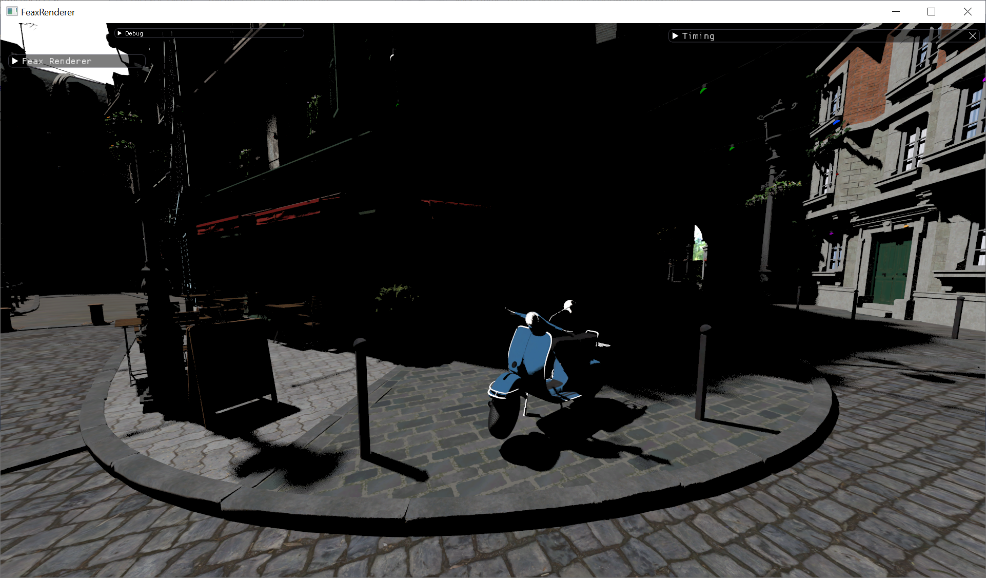
What if we stress it even more using a 6-64-64-64-1 MLP? In this case the compute shader inference costs 240.5ms, while the Tensor core one 1.39ms, a breathtaking 173x speedup. The screenshot above is actually from this large MLP.

The GPU trace of the large MLP inference show how much the Tensor cores light up

compared to the smaller 6-3-3-1 MLP case which barely utilises them.

Although, like discussed, RTAO encoding is probably not the best or most meaningful application for an MLP, this nevertheless shows that this technique could be viable from a performance standpoint using the Tensor cores for inference.

Of course it is worth mentioning that this large speedup is compared to an unoptimised compute shader that implements inference using float32 weights/biases reading them straight from VRAM, something that puts a lot of pressure on memory bandwidth and L2 throughput (right column below)

On the other hand, the Tensor core implementation has higher L1TEX throughput, likely because the cores use shared memory (which is stored in a part of the L1TEX cache) to store matrix data and overall higher SM throughput, completing work much faster.

There is a lot of room for improvement in the compute shader version though: using a smaller data type (eg float16) to store the MLP, shared memory to cache weights and reorganising the architecture to avoid reading the same data multiple times will bring down the cost but even if we managed to make it 10x faster the Tensor core acceleration capacity will remain impressive, especially for large networks.

The Cooperative Vectors feature in this form won’t officially be supported in a future Agility SDK, having been superseded by the Linear Algebra Matrix spec which in under review and will likely be released with SM6.10. In either case, the prospect of accessing Tensor cores from any HLSL shader is intriguing, given the range of opportunities it could unlock.

In recent years, neural networks have started to find their way into many areas of rendering. While antialiasing and upscaling are probably the most well‑known uses, they’re far from the only ones—texture compression, material representation, and indirect lighting are all active areas of research and development.

I recently started tinkering with neural networks, experimenting with small multilayer perceptrons (MLPs) as a way to encode data in the context of rendering. This post outlines the process and shares some of the initial results and observations from a graphics programmer’s perspective (without much previous experience in neural networks).

Before we begin, a quick note that this is not really a tutorial about MLPs, neural networks (NNs), even in their simplest form are a fairly complex topic and there are many good resources out there to start learning about them, I recommend these 2 as an introduction: Machine Learning for Game Developers and Crash Course in Deep Learning. Instead, I will summarise a few aspects of them for reference.

For a visual reference, this is what a simple MLP looks like:

In this case the network is made up of 3 input nodes, 2 hidden layers of 3 nodes each and one output node (From now on I will use the 3-3-3-1 notation to describe an MLP). The intermediate layers are “hidden” in the sense that we don’t interact with them directly, we only provide the input data and observe the output data. Also, I used this particular number of nodes in this configuration but there is no limit to the number of nodes in each layer, other than memory and processing time. And the number of nodes in a layer matters, because each node processes all the nodes of the preceding layer (i.e. the graph is fully connected), for example focusing on Node 0 in the hidden layer 1:

it will combine the 3 input nodes and produce its output (fed to the next layer) as follows

The output value of node 0 is simply put a biased weighted sum of all the input nodes output. Before we feed that value to the next layer we have to pass it through an “activation” function. This performs an operation on that value, a popular one being removing all negative values, called ReLU:

and a variation of it

for a small alpha value (eg 0.01). This version still keeps some negative outputs and I have found leads to faster learning. There are many options when it comes to selecting an activation function for a neural network, each having a different impact on the learning rate and convergence, ReLU and LeakyReLU are a good first starts though and LeakyReLU is what I used for the experiments described in this post.

Going back to the reference to storage requirements, to store the weights and biases for the above MLP, assuming a float data type for each, we would need for the first hidden layer 3 floats for the weights of the inputs and one float for the bias per node (3×3+3 floats), for the second the same amount and for the output 1×3+1 floats, so in total 28 floats to store the whole MLP. It easy to see that this can go up significantly, for an MLP with 9 input nodes, 3 hidden layers of 64 nodes and a 3 node output we would need 9155 float numbers to store. This can go down by using smaller data types, like fp16 or even lower for example.

Implementing an MLP to successively combine nodes and produce output like described above is very straightforward. What is tricky is to calculate the weights and biases used and this is where training of the neural network is needed. Going deep into training is outside the scope of this post, like mentioned there are many good tutorials out there. For some context though, at a high level, this is what is happening: We start with some random weights and biases and given an input vector, we calculate the output of the network (forward propagation, aka inference). The output will of course be wrong, so we calculate how much wrong it is (during training we need to know both the input and the expected, correct output of the network), calculating a gradient (difference) using a “loss” function. We then feed that gradient backwards into the network to adjust weights and biases (back propagation). Having adjusted the weights/biases, we try again feeding a new (or the same) input vector and calculating the output, finding the difference/gradient from the correct output and back propagating it through the network. The intention is, after having repeated this process many, many times, for the calculated output will be close to the expected output, i.e. the network will have “learned” the set of input to output mappings.

In terms of implementation, I assumed MLPs of a maximum of 5 layers, including the input and output layers (so a maximum of 3 hidden layers). The weights and biases I stored in 2 ByteAddressBuffers. Both inference and back propagation are loop heavy, to help the compiler a bit, similarly to this post, I defined number of layers and nodes per layer statically, avoiding dynamic loops. I won’t be adding too much code to the post, I’d suggest the reader has a look at the mentioned blog post which also includes a good sample but as an example, this is the code that returns the index into the weights and biases buffers based on layer index, node index and element (weight or bias) index:

#define MAX_LAYER_COUNT 5

static const uint neuronsPerLayer[MAX_LAYER_COUNT] =
{
    LAYER0_NEURON_COUNT, LAYER1_NEURON_COUNT, LAYER2_NEURON_COUNT, LAYER3_NEURON_COUNT, LAYER4_NEURON_COUNT
};

static const uint weightOffsetsPerLayer[MAX_LAYER_COUNT] =
{
    LAYER0_WEIGHT_OFFSET, LAYER1_WEIGHT_OFFSET, LAYER2_WEIGHT_OFFSET, LAYER3_WEIGHT_OFFSET, LAYER4_WEIGHT_OFFSET
};

static const uint biasOffsetsPerLayer[MAX_LAYER_COUNT] =
{
    LAYER0_BIAS_OFFSET, LAYER1_BIAS_OFFSET, LAYER2_BIAS_OFFSET, LAYER3_BIAS_OFFSET, LAYER4_BIAS_OFFSET
};

static const uint neuronOffsetsPerLayer[MAX_LAYER_COUNT] =
{
    LAYER0_NEURON_OFFSET, LAYER1_NEURON_OFFSET, LAYER2_NEURON_OFFSET, LAYER3_NEURON_OFFSET, LAYER4_NEURON_OFFSET
};

uint GetNeuronCount(uint layer)
{
    return neuronsPerLayer[layer];
}

uint GetWeightIndex(uint layer, uint neuronIndex, uint weightIndex)
{
    return weightOffsetsPerLayer[layer] + neuronIndex * neuronsPerLayer[layer-1] + weightIndex;
}

uint GetBiasIndex(uint layer, uint neuronIndex)
{
    return biasOffsetsPerLayer[layer] + neuronIndex;
}

uint GetNeuronIndex(uint layer, uint index)
{
    return neuronOffsetsPerLayer[layer] + index;
}

The inference code is like I mentioned is quite simple, made up of 3 nested loop as we need to iterate over the layers, the nodes of a layer and the inputs to the nodes.

void ForwardPass(inout float inputs[LAYER0_NEURON_COUNT], inout float nodeOutputs[MAX_NOOF_NODES])
{
    uint outputIndex = 0;
    
    //input layer
    for (uint index = 0; index < GetNeuronCount(0); index++)
    {
        nodeOutputs[outputIndex++] = inputs[index];
    }
    
    //rest of the layers
    for (uint layer = 1; layer < LAYER_COUNT; layer++)
    {
        for (uint index = 0; index < GetNeuronCount(layer); index++)
        {
            float output = GetBias(layer, index);
    
            for (int i = 0; i < GetNeuronCount(layer-1); i++)
            {
                float weight = GetWeight(layer, index, i);
                float previousLayerOut = nodeOutputs[GetNeuronIndex(layer - 1, i)];
                
                output += weight * previousLayerOut;
            }
        
            nodeOutputs[outputIndex++] = ActivationFunction(output);
        }
    }
}

The training phase broadly follows the above post again and I also implemented Adam optimisation to improve convergence.

Once I had the MLP implementation I started wondering where could I use it in the context of graphics. My approach was a bit simplistic, I focused on small MLPs with a low number of layers and nodes, with a single activation function for everything which is likely not the best way to get good results. The MLP output will depend on the number of layers, number of nodes per layer, activation function which could even be different per layer, loss function etc and to get good results one would need to experiment with all these, something that takes time due to the cost of training.

One interesting aspect of MLPs is that they can encode information/signals, in a similar way Spherical Harmonics, octahedral representations can, but in a non-analytical way, “learning” the expected output based on the input. As an example, I tried encoding the radiance from a cubemap along the normal direction. I used a minimal MLP of a 3-node input layer (normal xyz), one hidden layer of 3 nodes and a 3-node output layer (radiance rgb).

I also used an L2 Spherical Harmonics cubemap radiance encoding (using this great library) as a reference:

The SH approximation gives a general sense of radiance directionality but it is very coarse. The MLP described above on the other hand produces this output:

The directionality is much improved in this case, the output is like a very low resolution version of the cubemap. What is more interesting is that the L2 SH representation requires 27 floats (9 float3s) to store the coefficients, while that MLP needs 24 for a much improved quality.

Can the MLP be even smaller, what would happen if we reduce the hidden layer to 2 nodes?

and then to 1 node only?

With 2 nodes the output maintains the directionality broadly but introduces a colour shift which is undesirable. With one node it approximates the coarseness of the L2 SH representation closer, impressive for a mere 10 float storage requirement but the colour shifts will again make it unusable for radiance encoding applications.

Irradiance is also a directional quantity that can be encoded with an MLP. The output of a single hidden layer with 3 nodes NN looks as follows:

For comparison, this is the L2 Spherical Harmonics version

And this is the “ground truth” version, performing Monte Carlo integration of the cubemap in the shader.

Worth mentioning that the MLP is trained using the output of the ground truth irradiance calculation method. The MLP output is fairly close to the ground truth output, but not as close as the SH one, it appears that in the above scenario SH manages to encode irradiance slightly better.

A smaller MLP with a 1 node hidden later doesn’t manage to capture the directionality in the irradiance well.

One should never evaluate lighting techniques only on smooth spheres as this tends to hide issues that will become very obvious when a normal map is applied. For this reason, let’s rerun the above experiment adding a normal map to the sphere and zooming in a bit to see the result of each irradiance encoding approach.

The output of our small (1 hidden layer of 3 nodes) MLP is this

Along with the L2 SH output

And the ground truth output

Again, the Spherical Harmonics and Ground Truth outputs are quite similar, the difference of the MLP encoding become more pronounced though, the tiny MLP can’t encode irradiance directionality as well which can be seen as bounce light from the floor “leaking” on the faces of the bricks.

To cut a long story short, it appears that to get similar to SH response from the MLP, it needs to have 2 hidden layers of 4 nodes each:

Such an MLP would require 51 (floating point) numbers to store, which is quite a bit more than an L2 SH’s 27. In this context at least, it appears that a similar to an L2 SH, in terms of storage, MLP can encoding radiance better than irradiance.

Another signal I tried encoding is depth for a number of directions over a sphere centered at a world position (something that one could do with a depth cubemap as well), using raytracing to get the ground truth

The output of a 3-3-3-1 MLP, using a vector distributed over a sphere as an input is as follows

which is very coarse to be useful. Increasing the hidden layers to 3-32-32-32-1 we are beginning to discern features in the output:

And finally increasing to 3-128-128-128-1:

we can see many more details in the output and it is starting to become usable. An MLP of that size would need about 33,665 fp numbers for storage which is 134KB. For comparison a small, 128x128x6 depth cubemap is ~393KB. The MLP inference is very expensive though to make it useful using a compute shader implementation at least (44ms on an 3080 mobile GPU).

Another experiment I did was to test if an MLP could be used as an RTAO cache. In this case I used the world position and normal as input to a 6-32-32-32-1 NN (40ms)

Also increasing to 6-64-64-64-1 (240ms):

The MLP does a decent job of capturing AO at a world position for that view at a very large inference cost though. Also, didn’t try “teaching” the MLP multiple views due to training time, so it is not clear how suitable it is for learning the whole scene. For example, moving the camera to another view and spending the time to learn the AO, coming back to the original view the MLP struggles to remember the AO.

I am not sure if an MLP is capable of representing the whole scene AO accurately, I am assuming though a lot more training is needed and potentially a much larger network if this is the case. Even then the inference cost makes it less useful, at least for a compute shader implementation.

As a final test, I tried encoding a specular BRDF (Cook-Torrance). For that I went all in providing normal, light direction, view direction, F0 and roughness as inputs (13 in total) to the MLP. Although the inputs were selected randomly, I restricted light direction and view direction on the hemisphere centered on the normal to reduce the number of invalid combinations (eg light directions below the horizon which won’t contribute).

It turns out that the MLP really struggled to approximate the BRDF, even with a relatively large model 13-128-128-128-3

compared to the reference output

The same happened when I tried to reduce the inputs, removing F0 and roughness. It appears that the MLP (at least of that size for that amount of training) struggles to capture the specular lobe, especially for low roughness values.

Turns out there is a different parameterisation of a brdf, called the Rusinkiewicz parameterisation, popular in neural brdf implementations, which can reduce dimensional variation and improve specular lobe representation. In short, this approach reparameterises the brdf from the original normal vector reference (the origin of the brdf angles is the normal vector), to a half vector reference.

As a result the specular lobe lies mostly on the theta_h axis, irrespective of the value of theta_d. Also, for isotropic brdfs, like the one I am using, phi_h is zero reducing the input size even more.

Using the Rusinkiewicz parameterisation with 3 angles, theta_h, theta_d and phi_d, as input we manage to represent the specular lobe much better for a much smaller MLP 3-64-64-64-3 (output quality would likely increase with additional training time):

Even a smaller one, 3-32-32-3, seems to capture the specular lobe with some degree of accuracy although at a much increased training time and some extra quantisation visible.

Both the above examples assumed a fixed roughness and F0 which makes the MLP suitable for a single material only. Re-introducing F0 and roughness reduces the ability to capture the lobe, at least for the amount of training time I allowed, which was significantly longer than without those extra inputs.

To summarise the findings: neural networks, MLPs at least, are relatively easy to implement but tricky to get to produce useful results. Graphics programmers are used to tweaking parameters to fine tune systems and achieve better results but in this case, being a new area of me, I don’t feel I have a good grasp yet of what the impact of the various MLP parameters are, number of nodes vs numbers of layers and why one activation function is better than another. Training time is another factor, it takes a lot of time to see the outcome of any MLP alteration, especially for larger networks and the inference cost can also be quite high which may restrict real time rendering applications. I find this an interesting area though that shows promise as a way to encode/represent signals and the incoming HLSL support for inference acceleration has the potential to reduce the cost significantly.

Subdividing a 3D space into cells or voxels and using positional and/or directional information to directly index into it is a popular method to store and access local data, typically using 3D textures. This has been the basis of many global illumination algorithms, it is been used to store light lists, specular probes and decals that affect a world position as well as volumetric fog. Although it offers very fast access to the data, this approach has the disadvantage of sometimes requiring large amounts of memory something that can limit the coverage of the scene or require cascades of increasing cell size to keep the cost down.

An alternative to using cascades of 3D textures to store directly indexable data is a sparse representation using arrays instead of 3D textures and using a hash value derived from positional and/or directional (or other) data to produce indices to access the data, also known as spatial hashing.

To give this approach a try I did a quick implementation of a spatial hash structure and applied it to accelerate and reduce the noise of raytraced ambient occlusion inspired by this paper. The idea behind this is simple, RTAO only depends on the world position and the surface normal and for static scenes at least it is something that can be calculated, cached and reused. RTAO is calculated as normal, for example the output of 1 ray per pixel, randomly selected on a hemisphere, with a radius of 2 metres looks like this

In this scene, for every world position and every frame we keep recalculating the AO term although nothing really changes. Also, although the RTAO output goes through TAA in the above example it is still noisy and, to make matters worse, the noise is animated and needs a denoising step, typically both temporal (accumulation) and spatial (blurring) to improve the quality.

Instead of using the RTAO output directly, we can use the corresponding world position and normal to produce a hash value to index into an array that will store the output. Since allocating space to store every world position would be very expensive, we will quantise space creating cells that will accumulate AO for multiple, neighbouring world positions. Some programmer art to hopefully illustrate this:

Using a hash function h(x) with the position p of each world point as key we can produce a hash value H(p) as follows, using the “nested” approach:

Like discussed, we will quantise space introducing cells of size s to reduce storage requirements, so the hash value is calculated as

Adding the cell size to the hash value opens the door to implement lodding later. We also said that AO depends on both position and normal, so to properly index a cell we also need to add the normal to the hash value.

The value of sn used above is arbitrary, for quantisation. There is a large choice of functions that can produce the hash value we’ll use pcg as a good default option.

//https://www.shadertoy.com/view/XlGcRh
uint pcg(uint v)
{
    uint state = v * 747796405u + 2891336453u;
    uint word = ((state >> ((state >> 28u) + 4u)) ^ state) * 277803737u;
    return (word >> 22u) ^ word;
}

Assuming a hash map structure of size N, we can produce the index to access the cell for the specific world position and normal as such: H(p,n,s) % N.

Given that the hash map will be, out of necessity, restricted in terms of size, it is likely that conflicts will happen when different positions and normals produce the same hash value. To resolve a conflict first we need to identify it, for that reason we calculate another hash value from the position and normal and store it in the hash map when initialising a new cell to use as a checksum. Similarly to this post, we will use the xxhash32() function.

//https://www.shadertoy.com/view/XlGcRh
uint xxhash32(uint p)
{
    const uint PRIME32_2 = 2246822519U, PRIME32_3 = 3266489917U;
    const uint PRIME32_4 = 668265263U, PRIME32_5 = 374761393U;
    uint h32 = p + PRIME32_5;
    h32 = PRIME32_4 * ((h32 << 17) | (h32 >> (32 - 17)));
    h32 = PRIME32_2 * (h32 ^ (h32 >> 15));
    h32 = PRIME32_3 * (h32 ^ (h32 >> 13));
    return h32 ^ (h32 >> 16);
}

This way, when H(p,n,s) points us to a specific hash map location, we can use the checksum to confirm if the position and normal are valid or different to the ones this particular cell corresponds to.

On last thing we need to discuss is what happens when the checksums don’t match. There are a lot of approaches to resolve a conflict, in this implementation we will be using linear search (aka linear probing) in which when a conflict is detected neighbouring hashmap entries are inspected to find an empty cell (checksum equals zero). This method is fast because it is cache coherent but not does not offer the best distribution of hash values. From that perspective, a better option would be “rehashing” where a new hash value is created using the hashmap/cell index for example.

To see all these in code, this is the implementation of the SpatialHash insertion function, adapted from:

//Adapted from https://gboisse.github.io/posts/this-is-us/
uint SpatialHash_FindOrInsert(float3 position, float3 normal, float cellSize)
{
    // Inputs to hashing
    int3 p = floor(position / cellSize);
    int3 n = floor(normal * 3.0);
    
    cellSize *= 10000; // cellSize can be small and lead to more conflicts, multiply to increase range
    
    uint hashKey = pcg(cellSize + pcg(p.x + pcg(p.y + pcg(p.z + pcg(n.x + pcg(n.y + pcg(n.z)))))));
       
    uint cellIndex = hashKey % HASHMAP_SIZE;
          
    uint checksum = xxhash32(cellSize + xxhash32(p.x + xxhash32(p.y + xxhash32(p.z + xxhash32(n.x + xxhash32(n.y + xxhash32(n.z)))))));
    checksum = max(checksum, 1); // 0 is reserved for available cells
        
    // Update data structure
    for (uint i = 0; i < SEARCH_COUNT; i++)
    {                
        uint cmp;        
        InterlockedCompareExchange(hash[cellIndex], 0, checksum, cmp);
        
        if (cmp == 0 || cmp == checksum)
        {
               return cellIndex; 
        }
                         
        cellIndex++;

        if( cellIndex >= HASHMAP_SIZE)
            break;
    }

    return  0xFFFFFFFFu; // out of memory 
}

This pretty much implements what we have discussed so far, it uses pcg() and xxhash32() to calculate the hash value and checksum using nesting and linear search to locate an empty cell (checksum equals zero) or a cell with the same checksum. It will search a maximum of SEARCH_COUNT cells (10 in this case) and then it will stop reporting an out of memory result.

The code that does the actual raytracing and uses the spatial hash to store the RTAO output is as follows

// resources to store the hash and the cell payload
RWBuffer<uint>              hash : register(u1);
RWBuffer<uint>              spatialData : register(u3);

cellSize = 0.1;
uint cellIndex = SpatialHash_FindOrInsert(worldPos, normal, cellSize, rngState);

if ( cellIndex != 0xFFFFFFFFu )
{
	float2 rand = saturate(float2(rand01(rngState), rand01(rngState)));

	float3 rayDir = SampleHemisphere(rand.xy);

	rayDir = normalize(rayDir.x * tangent + rayDir.y * bitangent + rayDir.z * normal);

	RayDesc ray;
	ray.Origin = worldPos.xyz;
	ray.TMin = 0.01;

	ray.TMax = 2;
	ray.Direction = rayDir;
	
	uint occlusion = FindHit(Scene, ray);
	
	uint data = (occlusion << 16) + 1;

	InterlockedAdd(spatialData[cellIndex], data, originalData);
	
	originalOcclusion = originalData >> 16;
	originalNoofSamples = originalData & 0xFFFF;

	outputRT[screenPos] = float(originalOcclusion + occlusion) / float(originalNoofSamples + 1); 
}

The data that we store in the cell payload is the number of hits and the total number of rays. We pack them both in a uint, 16 bits each and use InterlockedAdd to add to the existing cell value. This is fine as long as both values stay within the 16bit uint range. In the end we use both those values to calculate the occlusion factor and output it so that we can see the result.

And this is the output of the RTAO pass using the spatial hash to store the occlusion, a radius of 2m and a cell size of 10cm:

First thing we notice is that the image is much less noisy (no denoising has taken place, only TAA) than the traditional RTAO output and in motion it is much more stable. On the other hand, although AO in the distance looks great, closer to the camera it looks very blocky. This is the result of using a constant cell size across the scene.

To improve this, we can calculate a cell size that varies with distance, adapting the formula from:

float ComputeCellSize(float d, float f, float Ry, float sp, float smin)
{	
    float h = d * tan(f * 0.5);
    float sw = sp * (h * 2.0) / Ry;

    //From https://history.siggraph.org/wp-content/uploads/2022/08/2020-Talks-Gautron_Real-Time-Ray-Traced-Ambient-Occlusion-of-Complex-Scenes.pdf 
    //s_wd = 2^(floor(log2(sw / smin))) * smin
    float exponent = floor(log2(sw / smin));
    float swd = pow(2.0, exponent) * smin;

    return swd;
}

This uses the vertical FOV f, the distance from the camera d, the vertical image resolution Ry, a user defined feature size in screen space sp and an arbitrarily small smin defining the smallest possible feature in world space.

To demonstrate this in action using a sp value of 10 pixels and a smin value of 0.4, and focusing on 2 cells projected on screen, one on the pillar on the right and one in the far distance, we can see that they appear roughly the same size, although in world space they cover very different in size areas.

Using this approach to calculate the cell size we can get much better distribution of sizes based on distance and the RTAO quality increases significantly. The following result is produced with sp = 3 and smin = 0.07 and a hashmap that can store 10M cells:

and a close up to see some more detail.

The above images are without any denoising, only TAA. Averaging RTAO results in cells works well as a denoising technique.

We have already hinted the caveat though, the hashmap capacity is limited and eventually it will run out of space. The selected hashing function, the way conflicts are solved as well as the cell size can affect when this happens but it is unavoidable, especially as the camera moves around as in more realistic scenarios.

In the above screenshot I showcase this flying the camera around, at some point I started seeing black cells, the result of the hashmap not managing to find an empty cell or a cell with the correct checksum.

To improve this, we will take cell age into account, removing cells that are “old” based on some threshold. Implementation-wise this will need another buffer (hashTime) to store the frame count when a cell was last used. The way the hashmap is updated in SpatialHash_FindOrInsert changes as such:

// Update data structure
for (uint i = 0; i < SEARCH_COUNT; i++)
{                
	uint cmp;        
	InterlockedCompareExchange(hash[cellIndex], 0, checksum, cmp);
	
	uint originalTime;
	if (cmp == 0 || cmp == checksum)
	{
		InterlockedExchange(hashTime[cellIndex], FrameIndex, originalTime);
		
		return cellIndex; 
	}
	
	originalTime = hashTime[cellIndex];
	if (FrameIndex - originalTime > 20)
	{
		uint original;
		InterlockedExchange(hash[cellIndex], checksum, original);
		InterlockedExchange(spatialData[cellIndex], 0, original);
		InterlockedExchange(hashTime[cellIndex], FrameIndex, originalTime);
	   
		return cellIndex;
	}
	
	cellIndex++;
	if (cellIndex >= HASHMAP_SIZE)
		break;       
}

While searching the hashmap, when we find a new cell or a cell with the correct checksum the current frame count is atomically stored in the hashTime buffer. This is the time that particular cell was last used. Else, as we look for appropriate cells in the neighbourhood, we check the time a cell was last used. If it is older that an amount of frames, we empty it and make it available to store RTAO data.

Performing the same flythrough test as above showcases how this approach can handle the hashmap running out of memory. To stress test it even more, I additionally reduced the hashmap capacity to 1M entries.

Storing the output of RTAO in the spatial hash reduces noise and increases stability as discussed, but also has another advantage for static scenes, it is possible to stop raytracing after a while and reuse the cached result only to calculate AO:

uint cellIndex = SpatialHash_FindOrInsert(worldPos, normal, cellSize);

worldPos = originalPos; 

if ( cellIndex != 0xFFFFFFFFu )
{
	uint originalData = spatialData[cellIndex];
	
	uint originalOcclusion = originalData >> 16;
	uint originalNoofSamples = originalData & 0xFFFF;
	
	if (originalNoofSamples < 500)
	{
		float2 rand = saturate(float2(rand01(rngState), rand01(rngState)));

		float3 rayDir = SampleHemisphere(rand.xy);

		rayDir = normalize(rayDir.x * tangent + rayDir.y * bitangent + rayDir.z * normal);

		RayDesc ray;
		ray.Origin = worldPos.xyz;
		ray.TMin = 0.01;

		ray.TMax = 2;
		ray.Direction = rayDir;
		
		uint occlusion = FindHit(Scene, ray);
		
		uint data = (occlusion << 16) + 1;

		InterlockedAdd(spatialData[cellIndex], data, originalData);
		
		originalOcclusion = originalData >> 16;
		originalNoofSamples = originalData & 0xFFFF;

		outputRT[screenPos] = pow(float(originalOcclusion + occlusion) / float(originalNoofSamples + 1), 1 );
	}
	else
		outputRT[screenPos] = pow(float(originalOcclusion) / float(originalNoofSamples), 1 );
}

Looking into the cell data for the given world position and normal, if the number of samples stored there is larger than a threshold, we can use the cell data and skip raytracing for that position.

As an example, selecting a pixel footprint value sp=5 and a 500 samples per cell threshold we can achieve this level of quality in 0.4ms

while the original RTAO approach costs 1.72ms

for a much lower quality and the need for additional denoising (both rendering on an Nvidia 3080 mobile GPU computing AO at 1080p). The extra memory required for the hashmap, cell times and cell payload buffers is about 11.4 MB (1M entries x 4 bytes x 3 buffers).

One last thing worth discussing: the cost as well as the quality of the spatial hash RTAO depends on the size of the cells as well as the amount of rays we cache in the cell. It may be the case that the output will need an amount of denoising as well if the quality is not good enough for the usecase.

There is a way to potentially reduce the need for denoising, and this is by jittering the world position used to index the cells:

float2 rand2 = saturate(float2(rand01(rngState), rand01(rngState)));
rand2 = 2 * (rand2 - 0.5);
worldPos += JitterScale * cellSize * (rand2.x * tangent + rand2.y * bitangent);

uint cellIndex = SpatialHash_FindOrInsert(worldPos, normal, cellSize);

The jitter happens on the tangent-bitangent plane and takes into account the cell size calculated at this distance. Also worth removing the jitter from the world position before raytracing else it may case artifacts.

The effect of this jittering is to randomly add the RTAO result of a particular cell to its neighbouring cells, which is the equivalent of spatial filtering but at no extra cost and can improve the quality significantly.

The approach discussed in this post only applies to a static scene, moving models will be the topic of a future investigation.

Following up on the previous post on GPU utilization and performance, and to provide a practical example, I expanded a bit on a topic discussed in brief: vertex shader exports and their impact on performance. To measure the performance cost, I set up a small experiment, rendering 250 instances of a model 10 times, each time increasing the number of vertex attributes by one until it reached a total of 10 float4 vertex exports, in addition to position export:

In an attempt to isolate the cost of the fixed function units and queues between vertex and pixel shader, I tried to keep vertex attributes (float4) exported simple on both ends, for example in the vertex the exports are nonsense and cheap to calculate:

#if NOOFEXPORTS > 1
	result.output1 = input.uv.xyxy / 2.0;
#endif

#if NOOFEXPORTS > 2
	result.output2 = input.normal.xyzz - 2;
#endif
	
#if NOOFEXPORTS > 3
	result.output3 = input.normal.xyzz/input.uv.x;
#endif	
	
#if NOOFEXPORTS > 4
	result.output4 = input.normal.xyzz + input.uv.xyxy;
#endif	

while on the pixel shader side they were cheap to use

#if NOOFEXPORTS > 1
	output.colour.rgba += input.output1;
#endif

#if NOOFEXPORTS > 2
	output.colour.rgba += input.output2;
#endif
	
#if NOOFEXPORTS > 3
	output.normal.rgba += input.output3;
#endif	
	
#if NOOFEXPORTS > 4
	output.colour.rgba += input.output4;
#endif	

Also, to keep the cost of pixel shading the same for each iteration, I cleared the depth buffer to reintroduce any overdraw. The pixel shader outputs to 2 rendertargets (G-buffer pass).

Low-level NVidia GPU architecture information online is limited, so, to help interpret the results, we will need to piece together how data flows between vertex shader and pixel shader using Nsight GPU trace and its documentation, the Nvidia forums and a few performance analysis posts linked at the end. Although I believe it is accurate, take the high level description below with a pinch of salt. If any of the assumptions is not correct please let me know.

As data is exported from the vertex shader, it is stored in the L1 memory of a SM, in a special allocation called ISBE. Next the Primitive Engine (PE) takes over, reading the data from ISBE and performing culling and clipping operations, eventually storing the data for the new/remaining triangle vertex attributes in L1 again, in another special allocation called TRAM to be used as pixel shader inputs. The GPU allocates 16KB of TRAM per SM and each attribute component takes up 12 bytes per triangle (sizeof(float) x 3), so a single float4 attribute exported by the vertex shader will take up 48 bytes per triangle, 10 float4s would take up 480 bytes per triangle. All ISBE, PE and TRAM can bottleneck data flowing between vertex to pixel shader and stall execution. We will later see manifestations of this as “Allocation” stalls, which refer to not enough memory being available to store data and “Fill” stalls, which are the result of upstream units that can’t fill the memory with data fast enough.

Running the experiment on a RTX 3080 mobile rendering at 1080p, the cost of the drawcall (in ms) as the number of float4 exports increases from 1 to 10 increases as follows:

The cost of the drawcalls between 1 and 10 float4 exports almost triples.

Using Nsight Graphics’ GPU Trace to determine how the allocations discussed above vary:

There is a noticeable increase in the amount of TRAM allocated as the number of float4 attributes exported increases (left to right). Taking the two ends, with 1 float4 export the first drawcall allocates 1,405 bytes per SM:

while with 10 float4 exports, the last drawcall allocates 4,646 bytes per SM.

Also the latter drawcall’s wave launch is stalled by TRAM fill measurably more than the former’s. This indicates that the Primitive Engine struggles to fill TRAM with vertex data and bottlenecks pixel shader execution. Comparing VPC, the PE unit that performs culling and clipping between one

and 10 vertex exports

the pressure on the VPC unit increases significantly, so it becomes more of a bottleneck, and that could possibly explain the TRAM fill warp stalls. Another interesting observation we can make is that the amount of traffic between the L1 and L2 caches increases significantly with the increased number of exports, which might indicate that VPC uses the L2 cache to store data, which is then copied to L1 (TRAM) before pixel shading.

The same is not true for ISBE allocation, which holds the vertex shader output, it looks about the same across all drawcalls

VTG refers to shaders processing geometry (vertex, tessellation, geometry). Comparing one float4 export

to 10 exports

we can confirm that the amount of memory allocated is about the same. The amount of vertex shader warps that stall due to ISBE memory space increases significantly as the number of vertex exports increases (stalls due failed allocation), so ISBE space becomes a bottleneck as well.

So, to summarise the a findings so far, it appears that as the number of exports increases, it puts pressure on Primitive Engine and the intermediate memory used to store the vertex attribute data and call stall both vertex and pixel shader execution that will explain the significant increase of the drawcall cost observed.

An interesting question is what happens if the pixel shader doesn’t use the vertex shader exports. For this, I just stripped out the relevant code from the pixel shader and only kept the vertex shader exports. In this case the drawcall cost remains the same regardless of the number of vertex shader exports. To quickly confirm checking the 2 extremes, one vertex shader export (float4)

and 10 vertex shader exports

The amount of TRAM allocated to store the pixel shader inputs is about the same. This indicates that the GPU knows that the vertex exports won’t be used and doesn’t allocate any extra space for them. Whether it is the shader compiler that strips out the unused exports from the vertex shader, or the hardware itself that doesn’t perform the allocations it is hard to say without access to the produced SASS, the shader ISA.

This behaviour is not consistent across GPU architectures from different vendors. I only have an integrated AMD GCN 5.0 GPU in my laptop, but running the same experiment the drawcall cost between runs remains exactly the same regardless of whether the pixel shader uses the vertex exports or not.

Also worth noting that the cost doesn’t increase as fast as on the Nvidia case with the number of vertex exports. It is not clear why there is drop in the cost for 2 exports, but Radeon profiler doesn’t seem to support GCN any more so I guess we’ll never know.

Going back to the main focus of this post, the Nvidia GPU architecture, if we change the exported data type from float4 to float, the drawcall cost as the number of export increases rises much slower, which is expected as the ISBE, PE and TRAM won’t be as much of a bottleneck any more:

Also comparing the amount of TRAM allocated when using float4 and float exports

we notice that it increases roughly linearly as well and we can see for example that the amount allocated for 8 float exports is about the same as 2 float4s. The linear increase also implies that export memory allocation has float and not float4 granularity (i.e., it allocates space for 3 floats if needed and does not round up to a float4).

To wrap up the investigation one more quick experiment, to interleave float and int exports as such

struct PSInput
{
    float output0 : TEXCOORD0;
	
#if NOOFEXPORTS > 1
	int output1 : TEXCOORD1;
#endif

#if NOOFEXPORTS > 2
	float output2 : TEXCOORD2;
#endif
	
#if NOOFEXPORTS > 3
	int output3 : TEXCOORD3;
#endif
}	

This is to determine if the GPU does any packing of floats and if mixing interpolated with non interpolated exports has any impact. It does not seem to make a measurable difference to the cost and intermediate memory allocated as the number of export increases though, which suggests that this particular GPU doesn’t handle float/int export or interpolation types any different.

To wrap up this quick investigation, this was a practical example of how fixed function units and intermediate memory storage can affect utilisation and rendering cost. Again, these findings might not generalise across different vendors’ GPUs, in some cases even across different architectures from the same vendor, so always profile to determine the actual impact with your rendering setup.

Further reads

• Optimizing DX12/DXR GPU Workloads using Nsight GPU Trace https://developer.download.nvidia.com/video/GDC-19/NSIGHT_GPU_TRACE_Bavoil.pdf
• The Peak-Performance-Percentage Analysis Method for Optimizing Any GPU Workload https://developer.nvidia.com/blog/the-peak-performance-analysis-method-for-optimizing-any-gpu-workload
• Life of a triangle – NVIDIA’s logical pipeline https://pixeljetstream.blogspot.com/2015/02/life-of-triangle-nvidias-logical.html

Drill deep into a GPU’s architecture and at its heart you will find a large number of SIMD units whose purpose is to read data, perform some vector or scalar ALU (VALU or SALU) operation on it and write the result out to a rendertarget or buffer. Those units can be found in what Nvidia calls Streaming Multiprocessors (SM) and AMD calls Workgroup Processors (WGP). Achieving good utilisation of the SIMD units and VALU throughput (i.e. keeping them busy with work) is critical for improving the performance of rendering tasks, especially in this era of increasingly wider GPUs with many SIMD units.

To read and write the data they operate on, the SIMD units interact with the rest of the GPU via a number of “fixed function” units, for example the TEX unit to serve data requests, the Register File to store temporary data (VGPRs), the ROP units to write to the rendertargets, a number of caches to store and read data from. This, for example, is the SM of Blackwell’s architecture, showcasing some of the units the VALU (FP32/INT32) units interact with (source):

The fixed function units are fast, due the simple nature of their work, but they can still become a bottleneck and starve the VALU units from work, or block it from writing the results out. For that reason, an important part of a graphics programmer’s job is analysing rendering workloads (drawcalls and dispatches) and trying to remove the bottlenecks caused by the fixed function units mentioned above and others like Input Assembler (IA), Raster units, but also memory bandwidth etc, that will reduce VALU utilisation.

Sometimes, due to the nature of the rendering work, the bottlenecks that reduce VALU utilisation/throughput are harder to remove, for example a shadowmap pass would be light on VALU work and bottlenecked more by the IA (World Pipe) and memory (VRAM) which feeds it vertex data, so the SM throughput (code execution) will be low:

Another example would be a compute shader pass that makes a copy of a rendertarget or creates a depth mipchain, where there just isn’t enough work in the shader to keep the VALU units busy. In such cases to achieve the best result, we need to take a step back and view the GPU performance holistically, focusing not on the performance of a single rendering task (drawcall/dispatch) but across rendering tasks and measure improvement across the whole frame. In this blog post I am discussing a few techniques that we can use to achieve that. A disclaimer: the effectiveness of any performance optimisation work depends a lot on the target GPU, the shader compiler, the renderer and the content rendered and is quite hard to generalise. As always, take any advice with a pinch of salt and always profile your use case.

Quick intermission to discuss bottlenecks a bit, I mentioned them a lot, but how can one identify what is actually the bottleneck and what needs going after? Profiling tools like Nsight Graphics (GPU Trace), AMD Radeon Profiler and PIX are all good options. Using a profiling tool, the easiest way is to visualise the bottleneck is to graph the utilisation of each GPU unit. In the case of GPU Trace, where the screenshot I posted above is from, it is the various “throughputs” plotted. With such a view, it is easy to see that, for example, the shadowmap pass is mostly bound (meaning it uses that unit/resource the most) by VRAM (memory bandwidth) and vertex input (World Pipe). The GTAO pass is bound by the L2 cache and the ShadowMask pass (which calculates raytraced shadows), by the RT cores. This means that if we want to improve the performance of any of those passes, the main bottleneck is first thing we should go after.

So, to begin with, it is worth stressing that we should first make every effort to reduce the cost/increase VALU utilisation of a single, expensive, drawcall wherever possible, targeting its specific bottlenecks. If for example a drawcall is memory latency bound, i.e. the VALU instructions are waiting for memory to arrive, increasing the occupancy by reducing VGPR (vector register) allocation, or reworking the shader in order to allow more instructions between memory read issue and memory use by, for example, partially unrolling a loop would be something worth trying. Also, increasing the flow of data to unblock VALU by packing/compressing shader input and output (this is true for all types of shaders, including vertex shader which the number of exported attributes could become a bottleneck on some GPUs) as well as observing data access patterns and adjusting the data structures used, for example a Structured Buffer will perform better than a Constant Buffer for random access on Nvidia GPUs, are things that will pay off.

If the nature of the bottleneck is such that further performance improvement is not easy, further gains could still be possible, but the approach might be counter-intuitive. For example if the occupancy of a shader is very high this could lead to cache thrashing as different in-flight waves are trying to access the cache. In such cases, lowering the occupancy by either increasing the VGPR allocation (creating a dummy large dynamic branch that never gets taken is one approach), or in case this is a compute shader by performing a dummy groupshared memory (LDS) allocation. LDS allocation to restrict occupancy is preferable if possible, because leaving VGPRs free could be beneficial to some other task running in parallel to this one (on the same graphics pipe but also with Async Compute, more on that later). Increasing the VGPR allocation though could have other, positive, effects, the compiler might take advantage of this and batch texture loads at the start of the shader to reduce memory latency.

Another thing worth considering is what the most suitable shader type for a specific workload is. A pixel shader is part of the GPU’s geometry processing pipeline which means that it depends on fixed function units for inputs (rasteriser and data exported by the Vertex Shader) and output, the ROP units to write to rendertargets, so it can get bottlenecked by either. A screen-space, export bound pixel shader (blocked by the ROP units), or a pixel shader that has divergent execution (i.e. an early out for some pixels in the warp/wave) could benefit more as a compute shader, which is lacking all those dependencies. Additionally, compute shaders have access to another type of memory, groupshared memory (or Local Data Store), which can be used as an intermediate storage to share data between threadgroup threads and speed up execution a lot.

On the other hand, the pixel shader pipeline might have fast paths and functionality in place that don’t exist for compute shaders. For example GCN has a dedicated cache (“Color cache”) in the Render Backend Unit to talk to the DRAM directly to read/write colour values, bypassing the L2 cache. This means that writing out to a rendertarget using a pixel shader might be faster than a compute shader as it frees up the L2 cache for other uses. This dedicated cache might not exist on other architectures though. A pixel shader can benefit from hardware VRS as well, reducing the cost, which is worth considering (although “software VRS” solutions are possible for compute shaders as well). Pixel shader output can be DCC compressed, something that might benefit memory bandwidth on subsequent reads of the rendertarget as a texture. Also, pixel shaders, full screen ones as well, can benefit from stencil operations, even depth operations, to speed up processing. Not spawning a wave is faster than spawning it an early-ing out (stopping shader execution due to a condition).

Work distribution differences between each shader type should also be factored in, when deciding where to move work to. For example, the GPU will allocate the whole threadgroup to a specific SM or WGP and all its warps/waves will be executed on the same SM/WGP. This is great for cache coherence and data locality purposes and can put the groupshared memory to good use, especially for large threadgroups. On the other hand large threadgroups need more resources (VGPRs/LDS) to be available before spawning it on a SM/WGP, which might introduce contention and delays. Pixel shader waves are spawned more predictably, in a tiled fashion based on screen location (source).

and might lead to faster execution. Moving VALU work to the vertex shader, to reduce pressure on a VALU bound pixel shader, is an option but it comes with caveats: cache coherence and data locality might not be great in a vertex shader due to the wave launch pattern (on GCN it is one per Compute Unit for eg), vertex shader work that is done for culled triangles/pixels is wasted and also exporting data from the vertex shader to the pixel can become a bottleneck on some GPU architectures. With current triangle counts and densities, moving work to the vertex shader might be less appealing.

On some architectures, where there is a choice of wave size like on RDNA, the shader type might impact execution and performance as well. On RDNA compute shaders are runnning with 32 threads per wave (wave32) and pixel shaders are running with 64 (wave64). A shader that relies heavily on wave intrinsics might benefit more as a wave64 pixel shader as it can get more work done (64 work items as opposed to 32). Also, wave intrinsics is a better way to share data between threads than the groupshared memory mentioned earlier as it is stored in VGPRs, the fastest storage available to the SIMD. On the other hand shaders with divergent execution, eg (stochastic) screen space reflections, might perform better as a wave32 compute shader, as the wave will have a higher chance to finish and retire earlier with less threads. Worth mentioning that since SM6.6 HLSL defines WaveSize for compute shaders, so that could be an option to increase the size as well, where supported.

Converting a workload to a compute shader has another potentially big advantage, it opens up the way for it to use Async Compute to run in parallel to graphics pipe work (i.e. overlap vertex or pixel shader or even other compute shader execution). Async compute is a great tool to increase VALU utilisation, as it can overlap other, potentially fixed function unit bottlenecked passes and use the resource they can’t use. For example, a cache and SM bottlenecked pass (GTAO),

can be paired well with an RT Core bound pass (Shadowmask)

to use GPU resource that the pass can’t use. Async compute could also overlap other passes with low VALU utilisation like a z-prepass or a shadow pass which likely will be mainly bottlenecked by geometry throughput, or a pixel shader export bound pass (screen space but also gbuffer fill potentially, depending on the complexity of the material shaders). A couple of things worth considering here, there is currently no API exposed way to control the execution of an async compute task, in terms of priority, throttling to reduce impact on the graphics pipe etc (on DirectX 12, Vulkan exposes VK_AMD_wave_limits I believe), so async compute can have a negative impact on the graphics pipe which might be ok, as long as the 2 tasks running in parallel cost less in total than when running serially on the graphics pipe. Dummy LDS (or, less preferably, VGPR as this is more likely to affect wave launch on the graphics pipe as well) allocations and threadgroup size can be used to affect execution of the async compute task as well, for example small threadgroups will likely overlap better than larger ones, and it will take some experimentation to find the the correct configuration you a particular use case. Finally, on the topic of compute shader overlap and on some GPU architectures, compute work on the graphics pipe can overlap pixel/vertex shader work as long as there are no barriers.

Removing the fixed function and other bottlenecks and allowing the GPU to perform useful work is critical in order to achieve good rendering performance and there are a lot of tools and techniques at our disposal to achieve that, be it single drawcall/dispatch optimisation or overlapping work to take advantage of unused compute resource, even if it comes at an increased cost for the individual rendering tasks. With the large variety of GPU architectures in the market it is tricky to determine which approach will work best though, and it will take some trial and error to decide what works best in each use case as not all approaches will perform equally well on all GPUs.

Further reading

• RDNA Performance Guide https://gpuopen.com/learn/rdna-performance-guide/
• Advanced shader programming on GCN https://gpuopen.com/download/GDC2017-Advanced-Shader-Programming-On-GCN.pdf
• Engine Optimization Hot Lap https://gpuopen.com/download/gdc_2018_sponsored_engine_optimization_hot_lap.pptx
• Advanced API Performance: Shaders https://developer.nvidia.com/blog/advanced-api-performance-shaders/
• Low-Level Optimizations in The Last of Us Part II https://s3.amazonaws.com/nd.images/research/2020_siggraph/Low_Level_Optimizations_In_TLOU2.pptx

GPUs make work parallelism very easy by design: each drawcall/dispatch shader instruction operates on batches of vertices, pixels, threads in general at the same time automatically. On the other hand, GPU work is pipelined, its architecture comprises various specialised (fixed function like input assembler, raster) and programmable (like Streaming Multiprocessor/SM) units connected by queues and depending on the nature of the work, a particular unit can become a bottleneck leaving the rest of the GPU underutilised.

We see this quite often in modern engines: rendering might start with some compute shader work to calculate a fluid simulation for example, followed by a GPU skinning pass both often memory and ALU bound, then by a shadow pass, a z-prepass maybe and a g-buffer pass, work that is mainly bottlenecked by geometry processing, i.e. vertex and triangle throughput. Then, for the rest of the frame the GPU transitions to more intensive pixel processing work, either with pixel or compute shaders, stressing again ALUs, caches and memory bandwidth.

My toy renderer is in no way representative of a AAA renderer, nevertheless, a GPU trace can give an example of this in practice:

The GPU units utilisation is very uneven, the shadow pass and the g-buffer pass put more pressure on the World Pipe (geometry processing) and VRAM to bring in vertices and textures while screen space lighting techniques like GTAO stress cache and ALU (SM) more. Often the GPU loads between passes are complementary and all passes underutilise some parts of the GPU, potentially leaving performance on the table.

To address this, IHVs have in the past few GPU generations, introduced the Asynchronous Computing (aka async compute, AMD) and Simultaneous Compute and Graphics (NVidia) technologies aimed to improve GPU utilisation by dispatching instructions from different tasks for SM execution, in parallel. This is achieved by separate hardware pipelines, graphics and compute, to submit to and schedule work.

Graphics APIs abstract the hardware pipelines using command queues (DirectX 12), there is one for graphics and compute work (graphics command queue) and one for compute work only (compute command queue). There is also a copy queue for data transfers but it is not relevant to this discussion. All the work we submit to a command queue via command lists, to implement for example techniques like shadowmap rendering, ends up being submitted to a hardware pipeline to be scheduled for execution. Unlike the graphics command queue, the compute queue only has access to units that involve shader execution (SM/caches) and not geometry processing, rasterisation and backend to write to rendertargets, i.e. it has less dependency on fixed function units. The idea is that overlapping work on multiple queues will increase GPU utilisation and improve performance.

Async compute is more of a scheduling mechanism, all tasks still target and compete for the same GPU resources (SM, caches, memory bandwidth). This means that based on how well we manage to pair tasks with the graphics queue will determine if async compute improves or worsens performance. For example pairing tasks that both are ALU bound, or memory bound may increase contention and possibly slow both down.

Let’s say that we want to move to async compute the GTAO (SSAO) technique in the GPU trace screenshot I shared above. The GTAO is cache first and ALU (SM) bound, while the raytraced shadows pass next to it is mainly RT core bound, it looks like pairing them is a good match.

Moving work to a compute queue is relatively straightforward, the first step is it create another command queue declaring it as “compute” only:

D3D12_COMMAND_QUEUE_DESC queueDesc = 
{ 
	D3D12_COMMAND_LIST_TYPE_COMPUTE, 
	D3D12_COMMAND_QUEUE_PRIORITY_NORMAL, 
	D3D12_COMMAND_QUEUE_FLAG_NONE 
};

m_device->CreateCommandQueue(&queueDesc, IID_PPV_ARGS(&m_computeCommandQueue));

Then we create command lists as normal and submit them to the compute queue for scheduling and async execution. There is one complication what needs special handling: once the work starts on the compute pipe, we need a way of knowing when it will finish. If the async task has any dependencies up stream, we need a way of knowing when they will be ready. In this particular case for example, GTAO needs the depth buffer and the normal buffer from the G-buffer pass so it can’t start before it finishes and downstream, the Composite pass needs to use the output of GTAO so it can’t start before GTAO finishes. The way to coordinate all this and work across GPU pipes in general is by using fences. Using a fence object the command queues can notify that a command list has finished execution by using the Signal() method, or wait for a command list to finish execution, using the Wait() method.

In the above case I set it up roughly as follows

// fences and values variables added here for reference
ComPtr<ID3D12Fence> m_toGraphicsFence; // to notify the graphics queue 
ComPtr<ID3D12Fence> m_toComputeFence; // to notify the compute queue
UINT64              m_toGraphicsFenceValue;
UINT64              m_toComputeFenceValue;
	
//create command list for gbuffer pass
RenderGBuffer();

if (m_state.AppSettings.AsyncCompute)
{
	// execute command list 
	m_commandList->Close());
	m_commandQueue->ExecuteCommandLists(1, CommandListCast(m_commandList.GetAddressOf()));
		
	// Add a signal command to the graphics queue to notify listeners
	m_commandQueue->Signal(m_toComputeFence.Get(), ++m_toComputeFenceValue));
}

// .. do other work

if (m_state.AppSettings.AsyncCompute)
{
	// wait for the GBuffer rendering work to finish
	m_computeCommandQueue->Wait(m_toComputeFence.Get(), m_toComputeFenceValues);
}

// create command list for GTAO
RenderGTAO();

if (m_state.AppSettings.AsyncCompute)
{
	// execute the command list on the compute pipe
	m_computeCommandList->Close());
	m_computeCommandQueue->ExecuteCommandLists(1, CommandListCast(m_computeCommandList.GetAddressOf()));

	// notify any listeners downstream when the work is done
	m_computeCommandQueue->Signal(m_toGraphicsFence.Get(), ++m_toGraphicsFenceValues));
}

// .. do other work

if (m_state.AppSettings.AsyncCompute)
{
	// execute command list 
	m_commandList->Close());
	m_commandQueue->ExecuteCommandLists(1, CommandListCast(m_commandList.GetAddressOf()));
	
    // wait for the signal for GTAO completion.
	m_commandQueue->Wait(m_toGraphicsFence.Get(), m_toGraphicsFenceValues);
}

//Create command list for composite pass
RenderComposite();

This is pretty much all that is needed to submit work to the 2 command queues and synchronise between them, effectively a command queue signals completion of a command list and the other command queue waits for that signal before it executes its own command list. Worth mentioning that Wait() is blocking on the GPU (but not on the CPU), work will stop on that command queue/hardware pipe until it gets the Signal() from the other command queue.

In a proper engine command list creation would be multithreaded and each pass would likely have its own command list. In my toy engine I use a single command list for graphics and another one for compute so to simplify things I close, execute and reuse them.

There is one more thing to consider, we talked about how the compute queue can’t see the fixed function units related to vertex and pixel shader execution. This has a knock on effect on resource transitions, a command list submitted to the command queue can’t transition a resource from states like D3D12_RESOURCE_STATE_RENDER_TARGET or D3D12_RESOURCE_STATE_PIXEL_SHADER_RESOURCE. Transitions like these need to happen on the graphics queue.

With this in place, let’s start reviewing some performance results. Here we see the outcome of GTAO running on the compute pipe with correct synchronisation using a fence (all costs refer to an NVidia 3080 mobile running at 1080p):

The task starts after the GBuffer pass has finished and runs in parallel to the raytraced shadows pass on the compute pipe. The throughput of the various units has improved and the GPU is now better utilised. GTAO and shadows when run serially take 5.73ms, while when GTAO runs async over the raytraced shadows, the combined cost is about 4.6ms a saving of more than a ms (it is slightly more as GTAO overlaps the hierarchical depth buffer pass a bit as well). Even if the pairing between these 2 tasks is good, there is still an impact on the cost of the individual tasks, they are both individually more expensive compared to when run serially on the graphics pipe, for example the GTAO cost increases from 1.97ms to 3.22ms. What really matters in this case though is the combined cost when run in parallel and this is the measure of success.

One thing worth checking is if running GTAO on the compute queue alone has any impact on its execution time.

Interestingly no, it takes the same amount of time when scheduled on the compute pipe and when running alone, indicating that there is nothing inherently limiting when running a task async, it is the contention for GPU resources that slows the 2 overlapped tasks down.

If by the time the downstream task needs to run a Signal() from the other command queue has been called with the appropriate fence value, Wait() doesn’t have an impact on the execution. If Signal() hasn’t be called and the correct fence value hasn’t been sent, GPU execution on the command queue will block, draining the hardware pipe from any work. To showcase this I made the raytraced shadows pass artificially faster and moved the Wait() right after it on the graphics queue.

We notice 2 things, first all work on the graphics pipe stops when the Shadowmask dispatch finishes as all subsequent work must Wait() for the correct fence value and this doesn’t happen until GTAO finishes, creating a bubble. This highlights a potential difficulty in scheduling async work with varying workloads on the graphics pipe, as they can finish earlier or later. Second, the GTAO cost is much smaller in this case compared to what it was when it fully overlapped the Shadowmask pass earlier, 2.3ms vs 3.22ms, which indicates that there is no static allocation/assignment of SMs to each task, and that the GPU can dynamically reallocate SMs to each hardware pipe as needed.

We talked about how correct pairing of tasks is of great importance and will determine the success of async compute and this is likely the harder to get right aspect of it. Focusing on SM (ALU) throughput alone is not enough, for example overlapping GTAO over a BRDF LUT dispatch that is SM bottlenecked, even though GTAO itself is ALU heavy:

leads to the combined pass of the 4 passes (Hierachical depth, GTAO, BRDF LUT and Shadowmap) dropping from 7ms down to 5.7ms, effectively giving us the BRDF pass for “free”:

Overlapping GTAO over other work that has both high SM and cache throughputs, such as the Generate Rays for RTGI and Lighting passes leads to somewhat reduced gains dropping the combined cost from 6.8ms (on the graphics pipe) to 6.1ms

Like discussed, the 2 command queues dispatch work in parallel, letting the tasks contest for GPU resources during execution. There is no good way to determine the priority of each tasks, there is a Priority field in D3D12_COMMAND_QUEUE_DESC which can be set to Normal or High but I found it to make no different on this GPU.

In the end it will take some experimentation to determine what works best in your case, comparing the main bottlenecks and SM occupancy for each pass and attempting and profiling combinations that reduce GPU resource contention to achieve the best possible utilisation.

For example, like I mentioned at the start of the post, the frame typically starts geometry bound, with shadowmap rendering pass, z-prepass and g-buffer pass usually bottlenecked by vertex and triangle processing and rasterisation. This is a good opportunity to overlap compute shader work to soak up all the unused SM. Since a lot of screen space lighting passes depend on the g-buffer output, swapping the order of shadow map rendering and g-buffer pass and overlapping this work over the shadowmap pass might be a good idea.

In this case overlapping GTAO, RTGI ray generation and BRDF LUT generation for good measure over the shadowmap rendering pass reduces the combined cost from to 6.63ms when running on the graphics pipe to 4.71ms when running async.

It also appears that GTAO is a better pairing for (rasterised) shadowmap rendering than raytraced shadows we examined earlier, finishing in 2.1ms as opposed to 3.22ms.

Although GPU are getting increasingly “wider”, capable of parallelising massive amounts of work, there will always be units to bottleneck execution and for that, async compute is something worth considering to fill-in those low utilisation moments. YMMV though depending on the engine architecture and rendering passes implemented as well as the targeted GPUs as their level of support for async compute may vary and will require experimentation to find which pairings work well for your case. It is also worth adding support for both async and non-async execution paths for a compute task to compare costs in each case and also for when improving the performance of a dispatch which should be done on the graphics queue, non-overlapping, to determine the real impact of the improvement work with no resource contention.

Further reads

• Advanced API Performance: Async Compute and Overlap https://developer.nvidia.com/blog/advanced-api-performance-async-compute-and-overlap/
• Deep Dive: Asynchronous Compute https://gpuopen.com/wp-content/uploads/2017/03/GDC2017-Asynchronous-Compute-Deep-Dive.pdf
• Breaking Down Barriers: An Intro to GPU Synchronization https://gpuopen.com/gdc-presentations/2019/gdc-2019-agtd5-breaking-down-barriers.pdf

Mesh shaders, introduced back in 2018 as an NVidia Turing and later as an AMD RDNA2 feature, is an evolution of the geometry pipeline which removes a number of fixed function units like the Input Assembler and Tessellator as well as the Vertex shader/Domain Shader/Geometry Shader stages and replaces them with a simpler, programmable pipeline consisting of an Amplification (aka Task) and a Mesh shader.

Ever since programmable shader GPUs were introduced a couple of decades ago, as I was just starting my graphics programming career, geometry and pixel processing, although becoming much more flexible using shaders, was supported by a number of fixed function units and caches that fetched and held data passed between the various stages of the pipeline. In the following high level view of the pipeline, the Input Assembler is responsible for setting up the vertices to feed to the vertex shader while the Primitive Assembler/Rasteriser are responsible for gathering the shaded vertices into triangles, performing out of screen, backface and small primitive culling and rasterising them to feed the pixel shader (green boxes are the fixed function units).

While the GPUs have become increasingly “wider” since, capable of many, many more shader calculations, the fixed function units remained and can become a bottleneck in some cases, especially with the increasing geometry complexity of the scenes in games.

Things changed with the introduction of mesh shaders, that shader (optionally combined with the amplification shader) is now responsible for reading and processing the geometry data and feeding it to the Primitive Assembler/Rasteriser stages, bypassing the Input Assembler:

Mesh shaders are like compute shaders in many ways, they spawn and work on threadgroups, using the DispatchMesh() API, and can use groupshared memory for intermediate data storing and sharing. Additionally, unlike the vertex shader pipeline that processes vertices in isolation, a mesh shader (as well as the amplification shader) has primitive awareness, individually and in clusters which offers the opportunity for finer grained primitive/cluster culling. Given the increasing complexity of game worlds, any opportunity to remove or reduce pressure on fixed function bottlenecks as well as for more efficient culling to avoid wasted work is very appealing.

Long overdue, I recently started tinkering with mesh shaders in my toy engine to get a feel for what is involved in adding support and any performance improvement opportunities. In this post I won’t go deep into mesh shader implementation, there are already a lot of good articles out there, I will focus more on the performance characteristics.

Let’s take a step back first and talk a bit about the importance of culling. In most cases, the expensive part of the rendering pipeline is pixel shading and the GPU is making a lot of effort not to shade pixels that are not visible. For that, it culls all out of screen (frustum), back-facing or small triangles that won’t contribute to the rendered image. This work is done through fixed function units, such as the Primitive Assembler (conceptually, individual GPUs vendors have different names for the fixed function units), which can become a bottleneck in some cases, especially when the pixel shader work is light, as in the case of a shadowmap rendering pass, or a z-prepass. All vertex shader work performed for vertices belonging to triangles that will eventually be culled is effectively wasted. For this reason, it is standard practice in games to test each model/mesh against the camera frustum and not render ones fully out of frustum (frustum culling). There is also the option to cull based on projected size on screen and even to cull occluded meshes (meshes behind other meshes) using a CPU-side solution. An additional benefit of culling a mesh, on the CPU, is that there is no need to submit it for rendering, avoiding all the overhead.

Culling can improve the rendering cost measurably, depending on the content and view, for eg this view from St Miguel scene

simple, per mesh, frustum culling alone drops the gbuffer pass cost from 3.11ms to 2.86ms, an 8% decrease. All the performance numbers quoted in this post refer to a RTX 3080 mobile GPU rendering at a 1080p resolution.

Culling at the mesh/model level on the CPU can be tricky though, developers try to adjust mesh sizes for culling efficiency (frustum/occlusion), splitting and batching meshes based on spatial proximity but even if a good balance is achieved for the main view between culling efficiency and rendering overhead, there could be other use-cases for example point light shadowmap rendering where the smaller frustum can lead to inefficient mesh culling.

Meshlets are another level of mesh subdivision, smaller chunks of the original geometry, usually ranging from 32 to 128 vertices, that can offer finer grained culling and can work well in different contexts. A quick showcase of this, the original scene rendered using a different colour per mesh

The same scene rendered using a different colour per meshlet (64 vertices per meshlet).

In the second view there are more opportunities for culling geometry, focus for example on the tree where in the original scene is a single mesh while on the meshlet scene is much more subdivided. Moving the camera closer and freezing visibility

with per mesh frustum culling we manage to cull little from the canopies

while with per meshlet culling most of the out of frustum canopy is culled.

This is all very convenient as meshlets is what mesh shaders process, which brings us to the topic of this post.

Adding mesh shader support is relatively straightforward, in its most basic form is an almost direct replacement of the vertex shader (the pixel shader remains the same). One of the ways the classic vertex shader pipeline differs to the mesh shader one is in the amount of work the fixed function units, the Input Assembler in particular, do in the background to deduplicate indices and prepare the data for consumption (I suggest reading this post for a discussion of this work in the context of the RDNA GPU architecture). None of this happens with the mesh shader pipeline which means that we need to do that work offline to convert the geometry data into meshlets, so that can be processed by the mesh shader.

To achieve this I used the meshoptimizer library that can both optimise the original meshes and create the meshlets needed by the mesh shader pipeline. The first thing I noticed after I added support for it to the toy engine is that meshoptimizer can improve the original meshes and can speed up the vertex shader pipeline as well. For example, testing with the St Miguel scene and view discussed above,

the original, unoptimised version costs 3.28ms, while the meshoptimizer optimised version costs 2.87ms (measuring gbuffer pass).

The improvement is content dependent, performing the same test with the Bistro scene

doesn’t really improve the cost, dropping it from 1.08ms to 1.05ms for the gbuffer pass, so as always it is worth profiling your specific use case.

Going back to mesh shaders, the meshlet related buffers the meshoptimizer produces, per mesh, are the following:

• a “mesh_vertices” buffer, which contains the deduplicated (unique) indices of the mesh vertices
• a “mesh_triangles” buffer, which contains the (triangle) indices to the mesh_vertices buffer
• a “meshlets” buffer which contains the vertex and triangle counts as well as the offsets to the mesh_vertices and mesh_triangles buffers.

and this is all that is needed to render the mesh using a mesh shader. The actual vertex data streams, eg positions, normals etc can be exactly the same as in the vertex shader pipeline. Worth noticing that there is an indirection here, mesh_vertices contains indices to the original vertex buffer and mesh_triangles contains indices to the indices in mesh_vertices. This may or may not be an issue and can be addressed by creating local vertex buffers for each meshlet at the expense of some vertex data duplication. It is also worth calling out that the original index buffer is no longer needed.

To get an idea of the overhead of a mesh shader pipeline, compared to the vertex shader one, when rendering the same content and the same, CPU side frustum culling, I started by trying a few meshlet/threadgroup size configurations in a “pass through” mode (no GPU side culling). This is the mesh shader I put together, for reference:

[NumThreads(MESH_SHADER_GROUPSIZE, 1, 1)]
[OutputTopology("triangle")]
void MSMain(
    uint gtid : SV_GroupThreadID,
    uint gid : SV_GroupID,
    out indices uint3 tris[MESHLET_MAX_TRIS],
    out vertices PSInput verts[MESHLET_MAX_VERTS]
)
{	
    PSInput result = (PSInput) 0;
	
    uint meshletIndex = gid;
    uint meshletCount = MaterialID >> 16;

    if (meshletIndex >= meshletCount)
        return;
	
    Meshlet meshlet = Meshlets[meshletIndex];

	//declare how many vertices and primitives we will be writing out 
    SetMeshOutputCounts(meshlet.VertCount, meshlet.PrimCount);
	
	//prepare and write out vertex data (AKA "vertex phase")
    int VertLoopCount = (MESHLET_MAX_VERTS + MESH_SHADER_GROUPSIZE - 1) / MESH_SHADER_GROUPSIZE;

    for (int i = 0; i < VertLoopCount; i++)
    {
        int index = gtid * VertLoopCount + i;
		
        // clamp index to the maximum number of vertices exported			
        index = min(index, meshlet.VertCount - 1);
                
		uint vertexIndex = MeshletVertices[meshlet.VertOffset + index];
		Vertex vertex = Vertices[vertexIndex];

		result.position = mul(World, float4(vertex.position.xyz, 1));
		result.worldPos = result.position.xyz;
		result.position = mul(ViewProjection, result.position);

		result.normal.xyz = mul((float3x3) WorldNormal, vertex.normal.xyz);
		result.normal.w = result.position.z;
		result.uv = vertex.texcoord;

		verts[index] = result;
    }
   
	// write out triangle indices (AKA "triangle phase")
    int PrimLoopCount = (MESHLET_MAX_TRIS + MESH_SHADER_GROUPSIZE - 1) / MESH_SHADER_GROUPSIZE;

    for (int i = 0; i < PrimLoopCount; i++)
    {
        int index = gtid * PrimLoopCount + i;
        
        //clamp index to maximum of primitives exported
        index = min(index, meshlet.PrimCount - 1);
		
		tris[index] = uint3(
						MeshletTriangles[meshlet.PrimOffset + index * 3],
						MeshletTriangles[meshlet.PrimOffset + index * 3 + 1],
						MeshletTriangles[meshlet.PrimOffset + index * 3 + 2]
						);
    }
}  

The above mesh shader is pretty standard: based on the maximum number of triangles, vertices and threadgroup size it decides whether to perform a loop in the shader to process input vertices and triangles. It is important to call SetMeshOutputCounts() at the start of the shader to declare the number of vertices and triangles to be written out. Writing out more vertices or triangles than those declared is undefined behaviour, the GPU is not required to clamp the numbers, so we need to protect against it in the shader. In many mesh shader examples online the usual way to achieve this is with a branch, eg

if (index < meshlet.VertCount)
{
     // process vertex
}

In my tests I found this to have a large overhead though due to divergence, so I ended up clamping the indices to the number of output vertices and triangles which was much faster although it could end up processing the same vertex/triangle multiple times (performance difference example below).

When setting up a mesh shader pipeline, 2 parameters are important and the trickiest to get right aspect of it, in than they may have dependencies on the content and the targeted GPU: the meshlet size and the mesh shader threadgroup size. According to the specification, a mesh shader can output a maximum of 256 vertices, a maximum of 256 triangles and have a maximum threadgroup size of 128.

There are a couple of things to consider when selecting the meshlet size an threadgroup size:

• The larger the meshlet (in terms of vertex count) the larger the vertex reuse (less need to shade a vertex multiple times)
• The smaller the meshlet the easier it is to cull
• Vertex shading the most expensive operation in the mesh shader, it might be preferable to make threadgroup size match meshlet vertex count to avoid wasted threads during the vertex phase.

In the following table I summarise the results of 2 experiments, trying different configurations of max number of vertices and max number of triangles per meshlet and mesh shader threadgroup size with and without a pixel shader bound, for the St Miguel scene, reporting the cost of the gbuffer and depth prepass.

A reminder that the vertex shader pipeline cost for the same view is 2.87 ms and with no pixel shader bound it is 2.42 ms.

In the above experiment I tried going as low as 32 vertices and 64 triangles per meshlet and as high as 128 vertices and 256 triangles. NVidia suggests using a max meshlet vertex count of 64 and a max triangle count of 126 (the number above is capped to 124 because meshoptimizer requires triangle counts multiples of 4). AMD recommends 128 vertices and 256 triangles. Also, I have tuned the threadgroup size based on the meshlet vertex count, as discussed above.

A first observation we can make is that for that specific scene and GPU, a mesh shader can match and maybe perform a bit better than the vertex shader pipeline for smaller meshlets. As the meshlet size increases we notice an increased overhead. It appears that 64 vertices/124 triangles/64 threads is the best configuration for this usecase. Interestingly, when no pixel shader is bound, in which case the vertex/mesh shader just outputs a position, the meshlet and threadgroup size don’t appear to matter as much and the vertex shader pipeline is faster than the mesh shader in all cases.

Quickly cycling back the the vertex/primitive index clamping discussed above, if we use a branch instead of the min(), the cost for the 124/64/64 case jumps from 2.78ms to 3.36ms.

To dig a bit deeper into what is happening under the hood, let’s compare 2 GPU Traces with (top) and without mesh shaders (bottom)

It is apparent that, not limited by the Primitive Distributor (PD, NVidia’s Input Assembler equivalent), the mesh shader version has noticeably higher “Geometry” warps (blue graph).

Comparing the 2 traces side by side (1st trace mesh shaders, 2nd trace vertex shaders), we can confirm that PD throughput is minimal compared the vertex shader pipeline and the Vertex Attribute Fetch (VAF, the unit that brings vertex data to the vertex shader) is not utilised at all, so those 2 units can’t bottleneck the mesh shader pipeline.

Inspecting the Vertex-Tessellation-Geometry (VGT), the stages related to vertex processing and shading, related counters we can confirm that the active warps per cycle have increased noticeably when using a mesh shader, about x6 the number.

This seems to also increase the pressure to the Inter-Stage Buffer Entry (ISBE) memory. This is where vertex data that flow through the VGT stages are stored. This in turn appears cause the mesh shader warp launch to be stalled more, compared to the vertex shader pipeline warps.

In overall, it appears that the mesh shader pipeline avoids the PD bottlenecks, utilises the geometry units better and has higher shader occupancy than the vertex shader pipeline.

Now that we’ve established that a mesh shader pipeline can have no overhead, or even slightly improve performance over a vertex shader pipeline in some scenarios, it is time to investigate the true potential of mesh shaders, visibility culling. Doing per triangle visibility calculations in the mesh shader is certainly possible but it is usually better to start at a coarser level to quickly cull geometry in batches and we already have the geometry is cullable batches, the meshlets. To process the meshlets we will need to add an amplification shader to the pipeline.

struct Payload
{
    uint MeshletIndices[AMPLIFICATION_SHADER_GROUP_SIZE];
};

groupshared Payload g_Payload;

[NumThreads(AMPLIFICATION_SHADER_GROUP_SIZE, 1, 1)]
void ASMain(
	uint gtid : SV_GroupThreadID, 
	uint dtid : SV_DispatchThreadID, 
	uint gid : SV_GroupID
)
{
    bool visible = false;
	
    if (dtid < MeshletCount)
    {
        // Do visibility testing for this meshlet
        visible =  IsVisible(MeshletCullData[dtid]);
    }
    
    // Compact visible meshlets
    if (visible)
    {
        uint index = WavePrefixCountBits(visible);
        g_Payload.MeshletIndices[index] = dtid;
    }

    // Dispatch the required number of threadgroups to render the visible meshlets
    uint visibleCount = WaveActiveCountBits(visible);
    DispatchMesh(visibleCount, 1, 1, g_Payload);
}

Quite similar to a mesh shader, or a compute shader for that matter, the amplification shader will process one whole meshlet per thread, determine visibility and if visible, store the meshlet index to the Payload, which is just some common to the whole threadgroup memory that will be passed down to the mesh shader. In this instance I used a threadgroup size of 32.

Meshoptimiser can also produce the culling data required for this, using meshlet_computeMeshletBounds(), in the form of bounding spheres for each meshlet, or cones for fast back face culling. In this instance I only used the bounding spheres for culling. In the first instance I tried some simple frustum culling, using the planes to determine visibility of the bound sphere:

bool IsVisible(CullData cullData)
{
	// Do a cull test of the bounding sphere against the view frustum planes.
    float4 centre = mul(World, float4(cullData.BoundingSphere.xyz, 1) );
    float radius = WorldScale * cullData.BoundingSphere.w;

    for (int i = 0; i < 6; ++i)
    {
        if (dot(centre, Planes[i]) > radius)
        {
            return false;
        }
    }
 
	return true;
}

For the reference St Miguel view, meshlet frustum culling makes a noticeable difference, dropping the g-buffer pass from 2.75ms (with CPU only, per mesh frustum culling) to 2.43ms. It is worth mentioning that this scene is made up of large triangles which cause some meshlets and bounding spheres to be very large, making them less effective during culling. More subdivision, or using bounding boxes instead of spheres might lead to improved culling.

To try a different culling method, I also dropped a quick and dirty occlusion culling implementation, based on an earlier experiment I described in this post. For a hierarchical z-buffer I used the one produced by FidelityFX SSSR I had already integrated to the toy engine. The occlusion culling code was used mostly verbatim from that post so I won’t be pasting it here, only the results.

Red pixels in the following screenshot represent meshlets that are occlusion pass in the amplification shader culled.

In terms of performance, meshlet occlusion culling makes a much bigger difference dropping the gbuffer pass cost (for that view) from 2.75ms (with CPU per mesh frustum culling) to 1.86 ms. Adding per meshlet frustum culling on top, drops it even further, to 1.64ms, offering in total a very respectable 40% cost decrease for that pass, view and content.

The culling numbers presented are using a meshlet size of 124 triangles and 64 vertices (and a threadgroup size of 64), which as discussed earlier seems to be the optimal meshlet size for this GPU and scene. We discussed above the meshlet size may have an impact on visibility calculations. To showcase this, I re-run the experiment using meshlets of 64 triangles, 32 vertices and a threadgroup size of 32. Although without an amplification shader and meshlet occlusion this meshlet size is not the best in terms of performance, things change when meshlet occlusion is factored in. In this case, the smaller meshlet has the advantage, dropping the overall cost of the mesh shader path further, to 1.59ms.

Comparing occlusion for both meshlet sizes (left 64 vertices, right 32) reveals noticeably increased occlusion when using the smaller meshlet.

If we compare this final cost to the original, vertex shader pipeline cost of 2.85ms, the mesh shader pipeline, with per meshlet frustum and occlusion culling, dropped the gbuffer pass cost by 44% for that scene and view.

Using the Bistro scene with the view showcased earlier, the same mesh shader configuration drops the g-buffer pass cost from 1.06ms to 0.74ms a 30% decrease, which speaks to the content dependent effectiveness of the new pipeline.

Let’s do another GPU trace comparison between the vertex shader pipeline and the mesh shaders pipeline implementing the occlusion culling techniques discussed to see where the improvements are, for the St Miguel view. Remember that one of the goals of this work was to reduce the pressure on the Primitive Assembler/Rasteriser units by “software” culling as much geometry as possible. We can see that, indeed, we managed to do so (1st trace is mesh shaders, 2nd trace is vertex shaders):

The VPC unit responsible for clipping and culling triangles before rasterisation processes many less using the mesh shader pipeline.

The ZCULL unit, responsible for coarse z-culling of pixels, now culls many less due to the occlusion culling in the amplification shader:

During geometry processing (VTG units), the mesh shader manages to spawn many more warps compared to the vertex shader pipeline, more pixel warps and improves utilisation of the Streaming Multiprocessor (SM, the unit executing the shaders) reducing the amount of unallocated warps, meaning that in overall the GPU manages to do more actual work.

There is one last thing to test, we discussed earlier that a “pass-through” mesh shader pipeline (no AS), was a bit more expensive than the original vertex shader one for all meshlet configurations for a depth only pass (eg shadowpass, z-prepass). Factoring in occlusion and re-running the z-prepass in St Miguel showcases a big drop in the cost from 2.41ms with vertex shaders to 1.24ms with an amplification shader and occlusion, around 48%, even larger than the g-buffer pass improvement.

Worth mentioning that meshlet, even triangle, culling is certainly possible using a traditional pipeline, Frostbite demonstrated a few years ago a compute shader pipeline, using execute indirect, that processed meshlets and performed a similar job. Mesh shaders is a more flexible pipeline though, easier to set up, no compaction needed to remove empty drawcalls, and culling is done “inline” without the need for a memory roundtrip to store the data and for barriers to correctly synchronise the work.

To summarise the findings, with the small sample of scenes I tried, mesh shaders appear have the potential to speed up rendering measurably. Their efficiency depends a lot on the rendered content though and it takes some experimentation to find what configuration (meshlet size/threadgroup size) will work best in each case. Removing the Input Assembler (IA) from the pipeline can allow the GPU to go wider when processing vertices in those passes where IA is the bottleneck and while it doesn’t remove the Primitive Assembler, it can reduce the pressure on it by culling meshlets and triangles that don’t contribute to the scene.

There are aspects of mesh shading like how to support instancing, lodding and how to compress the data output from the mesh shader that I haven’t talked about but this will likely be a topic for a future post.

Further readings on Meshlets and Mesh Shaders

• Reinventing the Geometry Pipeline: Mesh Shaders in DirectX 12
• Advanced Mesh Shaders
• Introduction to Turing Mesh Shaders
• Mesh and task shaders intro and basics
• Mesh Shaders in AMD RDNA 3 architecture
• Mesh shaders on AMD RDNA graphics cards
• Meshlet size tradeoffs
• Using Mesh Shaders for Professional Graphics
• Mesh Shader DirectX specification

I posted a few days ago a screenshot of the long shader ISA code produced by the RGA compiler for a single atan2() instruction. The post got quite a large engagement and it felt like a lot of people were surprised by the fact, so I decided to write a post to discuss the “hidden” cost of shader instructions a bit more.

For the following I am referring to GCN/RDNA architectures and most ISA was produced using https://godbolt.org/. To aid the discussion I have, quite unscientifically, assigned the cause of the “hidden” the cost of shader instructions broadly 3 to categories:

• No hardware support for the instruction
• Hardware implementation of the instruction
• Instruction has a dependency on a resource

Let’s start with the first category, an instruction doesn’t have a hardware (native) implementation and needs to be implemented using a, sometimes large, number of native instructions. This is very common cause of “hidden” cost and can take people by surprise. Inverse trigonometric functions (acos, asin, atan, atan2) don’t have a native implementation, this is for eg the RDNA ISA code produced for a single atan2:

  v_cmp_gt_f32 s[0:1], v2, 0 // 00000000001C: D4040000 00010102
  s_mov_b64 s[2:3], exec // 000000000024: BE82047E
  v_cmpx_eq_f32 exec, v0, 0 // 000000000028: D412007E 00010100
  v_mov_b32 v0, lit(0x3fc90fda) // 000000000030: 7E0002FF 3FC90FDA
  v_cndmask_b32 v0, lit(0xbfc90fda), v0, s[0:1] // 000000000038: D5010000 000200FF BFC90FDA
  s_andn2_b64 exec, s[2:3], exec // 000000000044: 8AFE7E02
  s_cbranch_execz label_0308 // 000000000048: BF8800AF
  v_cmp_gt_f32 s[4:5], v0, 0 // 00000000004C: D4040004 00010100
  s_mov_b64 s[6:7], exec // 000000000054: BE86047E
  v_cmpx_eq_f32 exec, v2, 0 // 000000000058: D412007E 00010102
  v_cndmask_b32 v0, lit(0x40490fda), 0, s[4:5] // 000000000060: D5010000 001100FF 40490FDA
  s_andn2_b64 exec, s[6:7], exec // 00000000006C: 8AFE7E06
  s_cbranch_execz label_0308 // 000000000070: BF8800A5
  s_mov_b64 s[8:9], exec // 000000000074: BE88047E
  v_cmpx_gt_f32 exec, abs(v0), abs(v2) // 000000000078: D414037E 00020500
  v_div_scale_f32 v1, vcc, v0, v0, v2 // 000000000080: D56D6A01 040A0100
  s_cbranch_execz label_01A4 // 000000000088: BF880046
  v_div_scale_f32 v3, vcc, v2, v0, v2 // 00000000008C: D56D6A03 040A0102
  s_denorm_mode 0x000f // 000000000094: BFA5000F
  v_rcp_f32 v6, v1 // 000000000098: 7E0C5501
  v_fma_f32 v5, -v1, v6, 1.0 // 00000000009C: D54B0005 23CA0D01
  v_fmac_f32 v6, v5, v6 // 0000000000A4: 560C0D05
  v_mul_f32 v4, v3, v6 // 0000000000A8: 10080D03
  v_fma_f32 v5, -v1, v4, v3 // 0000000000AC: D54B0005 240E0901
  v_fmac_f32 v4, v5, v6 // 0000000000B4: 56080D05
  v_fma_f32 v3, -v1, v4, v3 // 0000000000B8: D54B0003 240E0901
  s_denorm_mode 0x000c // 0000000000C0: BFA5000C
  v_div_fmas_f32 v1, v3, v6, v4 // 0000000000C4: D56F0001 04120D03
  v_mov_b32 v4, lit(0xbc8bf91a) // 0000000000CC: 7E0802FF BC8BF91A
  v_div_fixup_f32 v0, v1, v0, v2 // 0000000000D4: D55F0000 040A0101
  v_cmp_eq_f32 s[10:11], abs(v0), 0 // 0000000000DC: D402010A 00010100
  v_rcp_f32 v1, abs(v0) // 0000000000E4: D5AA0101 00000100
  v_and_b32 v2, lit(0x7fffffff), v0 // 0000000000EC: 360400FF 7FFFFFFF
  v_cmp_gt_f32 vcc, abs(v0), 1.0 // 0000000000F4: D404016A 0001E500
  v_and_b32 v0, lit(0x80000000), v0 // 0000000000FC: 360000FF 80000000
  v_cndmask_b32 v1, v1, 0, s[10:11] // 000000000104: D5010001 00290101
  v_cndmask_b32 v3, v2, v1, vcc // 00000000010C: 02060302
  v_mul_legacy_f32 v1, v3, v3 // 000000000110: 0E020703
  v_fmac_legacy_f32 v4, lit(0x3b47bf1d), v1 // 000000000114: 0C0802FF 3B47BF1D
  v_fma_legacy_f32 v4, v4, v1, lit(0x3d3751b7) // 00000000011C: D5400004 03FE0304 3D3751B7
  v_fma_legacy_f32 v4, v4, v1, lit(0xbd9e0bf8) // 000000000128: D5400004 03FE0304 BD9E0BF8
  v_fma_legacy_f32 v4, v4, v1, lit(0x3ddc5c26) // 000000000134: D5400004 03FE0304 3DDC5C26
  v_fma_legacy_f32 v4, v4, v1, lit(0xbe11cde3) // 000000000140: D5400004 03FE0304 BE11CDE3
  v_fma_legacy_f32 v4, v4, v1, lit(0x3e4cc636) // 00000000014C: D5400004 03FE0304 3E4CC636
  v_fma_legacy_f32 v4, v4, v1, lit(0xbeaaaaa3) // 000000000158: D5400004 03FE0304 BEAAAAA3
  v_fma_legacy_f32 v2, v4, v1, 1.0 // 000000000164: D5400002 03CA0304
  v_mul_legacy_f32 v4, v3, v2 // 00000000016C: 0E080503
  v_fma_legacy_f32 v1, -v3, v2, lit(0x3fc90fdb) // 000000000170: D5400001 23FE0503 3FC90FDB
  v_cndmask_b32 v1, v4, v1, vcc // 00000000017C: 02020304
  v_xor_b32 v0, v0, v1 // 000000000180: 3A000300
  v_mov_b32 v1, lit(0x40490fda) // 000000000184: 7E0202FF 40490FDA
  v_cndmask_b32 v1, lit(0xc0490fda), v1, s[0:1] // 00000000018C: D5010001 000202FF C0490FDA
  v_add_f32 v1, v0, v1 // 000000000198: 06020300
  v_cndmask_b32 v0, v1, v0, s[4:5] // 00000000019C: D5010000 00120101
label_01A4:
  s_andn2_b64 exec, s[8:9], exec // 0000000001A4: 8AFE7E08
  s_cbranch_execz label_0308 // 0000000001A8: BF880057
  s_mov_b64 s[10:11], exec // 0000000001AC: BE8A047E
  v_cmpx_eq_f32 exec, abs(v0), abs(v2) // 0000000001B0: D412037E 00020500
  v_mov_b32 v0, lit(0x3f490fda) // 0000000001B8: 7E0002FF 3F490FDA
  v_mov_b32 v1, lit(0xbf490fda) // 0000000001C0: 7E0202FF BF490FDA
  v_cndmask_b32 v0, lit(0x4016cbe4), v0, s[4:5] // 0000000001C8: D5010000 001200FF 4016CBE4
  v_cndmask_b32 v1, lit(0xc016cbe4), v1, s[4:5] // 0000000001D4: D5010001 001202FF C016CBE4
  v_cndmask_b32 v0, v1, v0, s[0:1] // 0000000001E0: D5010000 00020101
  s_andn2_b64 exec, s[10:11], exec // 0000000001E8: 8AFE7E0A
  v_div_scale_f32 v1, vcc, v2, v2, v0 // 0000000001EC: D56D6A01 04020502
  s_cbranch_execz label_0308 // 0000000001F4: BF880044
  v_div_scale_f32 v3, vcc, v0, v2, v0 // 0000000001F8: D56D6A03 04020500
  s_denorm_mode 0x000f // 000000000200: BFA5000F
  v_rcp_f32 v6, v1 // 000000000204: 7E0C5501
  v_fma_f32 v5, -v1, v6, 1.0 // 000000000208: D54B0005 23CA0D01
  v_fmac_f32 v6, v5, v6 // 000000000210: 560C0D05
  v_mul_f32 v4, v3, v6 // 000000000214: 10080D03
  v_fma_f32 v5, -v1, v4, v3 // 000000000218: D54B0005 240E0901
  v_fmac_f32 v4, v5, v6 // 000000000220: 56080D05
  v_fma_f32 v3, -v1, v4, v3 // 000000000224: D54B0003 240E0901
  s_denorm_mode 0x000c // 00000000022C: BFA5000C
  v_div_fmas_f32 v1, v3, v6, v4 // 000000000230: D56F0001 04120D03
  v_mov_b32 v4, lit(0xbc8bf91a) // 000000000238: 7E0802FF BC8BF91A
  v_div_fixup_f32 v0, v1, v2, v0 // 000000000240: D55F0000 04020501
  v_cmp_eq_f32 s[4:5], abs(v0), 0 // 000000000248: D4020104 00010100
  v_rcp_f32 v1, abs(v0) // 000000000250: D5AA0101 00000100
  v_and_b32 v2, lit(0x7fffffff), v0 // 000000000258: 360400FF 7FFFFFFF
  v_cmp_gt_f32 vcc, abs(v0), 1.0 // 000000000260: D404016A 0001E500
  v_and_b32 v0, lit(0x80000000), v0 // 000000000268: 360000FF 80000000
  v_cndmask_b32 v1, v1, 0, s[4:5] // 000000000270: D5010001 00110101
  v_cndmask_b32 v3, v2, v1, vcc // 000000000278: 02060302
  v_mul_legacy_f32 v1, v3, v3 // 00000000027C: 0E020703
  v_fmac_legacy_f32 v4, lit(0x3b47bf1d), v1 // 000000000280: 0C0802FF 3B47BF1D
  v_fma_legacy_f32 v4, v4, v1, lit(0x3d3751b7) // 000000000288: D5400004 03FE0304 3D3751B7
  v_fma_legacy_f32 v4, v4, v1, lit(0xbd9e0bf8) // 000000000294: D5400004 03FE0304 BD9E0BF8
  v_fma_legacy_f32 v4, v4, v1, lit(0x3ddc5c26) // 0000000002A0: D5400004 03FE0304 3DDC5C26
  v_fma_legacy_f32 v4, v4, v1, lit(0xbe11cde3) // 0000000002AC: D5400004 03FE0304 BE11CDE3
  v_fma_legacy_f32 v4, v4, v1, lit(0x3e4cc636) // 0000000002B8: D5400004 03FE0304 3E4CC636
  v_fma_legacy_f32 v4, v4, v1, lit(0xbeaaaaa3) // 0000000002C4: D5400004 03FE0304 BEAAAAA3
  v_fma_legacy_f32 v2, v4, v1, 1.0 // 0000000002D0: D5400002 03CA0304
  v_mul_legacy_f32 v4, v3, v2 // 0000000002D8: 0E080503
  v_fma_legacy_f32 v1, -v3, v2, lit(0x3fc90fdb) // 0000000002DC: D5400001 23FE0503 3FC90FDB
  v_cndmask_b32 v1, v4, v1, vcc // 0000000002E8: 02020304
  v_xor_b32 v0, v0, v1 // 0000000002EC: 3A000300
  v_sub_f32 v1, lit(0x3fc90fda), v0 // 0000000002F0: 080200FF 3FC90FDA
  v_sub_f32 v0, lit(0xbfc90fda), v0 // 0000000002F8: 080000FF BFC90FDA
  v_cndmask_b32 v0, v0, v1, s[0:1] // 000000000300: D5010000 00020300
label_0308:
  s_mov_b64 exec, s[2:3] // 000000000308: BEFE0402
  v_cvt_pkrtz_f16_f32 v2, v0, 0 // 00000000030C: D52F0002 00010100
  v_mov_b32 v3, 0 // 000000000314: 7E060280
  exp mrt0, v2, v2, v3, v3 done compr vm // 000000000318: F8001C0F 00000302
  s_endpgm // 000000000320: BF810000

Admittedly this is one of the most extremes examples, not all inverse trigonometric functions expand to so many instructions. It is not only inverse trigonometric instructions that are expanded into many native ones, tan() has no native implementation as well, it is calculated using cos and sin instructions, which have:

v_mul_f32 v0, 0.15915494, v0 // 000000000014: 100000F8
v_cos_f32 v1, v0 // 000000000018: 7E026D00
v_sin_f32 v0, v0 // 00000000001C: 7E006B00
v_rcp_f32 v1, v1 // 000000000020: 7E025501
v_mul_legacy_f32 v0, v0, v1 // 000000000024: 0E000300

More widely used instructions that don’t have native implementation are normalize() and length(), for eg this is normalize():

v_mul_legacy_f32 v1, v2, v2 // 000000000024: 0E020502
v_fmac_f32 v1, v3, v3 // 000000000028: 56020703
v_fmac_f32 v1, v0, v0 // 00000000002C: 56020100
v_rsq_f32 v1, v1 // 000000000030: 7E025D01
v_mul_legacy_f32 v2, v2, v1 // 000000000034: 0E040302
v_mul_legacy_f32 v3, v3, v1 // 000000000038: 0E060303
v_mul_legacy_f32 v0, v0, v1 // 00000000003C: 0E000300

Integer division using vector registers is another area of large instruction expansion. As there are no native vector instructions to implement this, a single x/y division with integer operands would produce around 35 instructions on RDNA ISA. Integer division with scalar registers is even worse, producing a mix of around 42 scalar and vector instructions (I will spare you from pasting unending streams of instructions here, you can experiment with godbold.org if you’d like to see it in action).

Cubemap sampling is another instruction that is, perhaps unexpectedly, expanded to multiple ones as the compiler is attempting to calculate the face to use:

// cubemap.Sample(samplerLinear, direction.xyz);  

v_cubema_f32 v1, v2, v3, v0 // 000000000034: D5470001 04020702
s_load_dwordx8 s[4:11], s[0:1], null // 00000000003C: F40C0100 FA000000
s_load_dwordx4 s[0:3], s[0:1], 0x000020 // 000000000044: F4080000 FA000020
v_cubetc_f32 v4, v2, v3, v0 // 00000000004C: D5460004 04020702
v_rcp_f32 v1, abs(v1) // 000000000054: D5AA0101 00000101
v_cubesc_f32 v5, v2, v3, v0 // 00000000005C: D5450005 04020702
v_cubeid_f32 v0, v2, v3, v0 // 000000000064: D5440000 04020702
v_fmaak_f32 v2, v4, v1, lit(0x3fc00000) // 00000000006C: 5A040304 3FC00000
v_fmaak_f32 v1, v5, v1, lit(0x3fc00000) // 000000000074: 5A020305 3FC00000
s_and_b64 exec, exec, s[12:13] // 00000000007C: 87FE0C7E
s_waitcnt lgkmcnt(0) // 000000000080: BF8CC07F
image_sample v[0:2], [v1,v2,v0], s[4:11], s[0:3] dmask:0x7 dim:SQ_RSRC_IMG_CUBE // 000000000084: F080071A 00010001 00000002

Another example of an HLSL operation that can have a large impact on number of instructions produced is register (VGPR) array indexing. Say that you try to access a register using a uniform (same for all threads) index:

 // float data[4] = {....} // store some values in a VGPR array
 // float result = data[index]; // index is the same for all threads 

  v_mov_b32 v4, 0 // 00000000004C: 7E080280
  s_cmp_lt_u32 s0, 4 // 000000000054: BF0A8400 <---- Protect against array overflow
  s_cbranch_scc0 label_0064 // 000000000058: BF840002 
  s_mov_b32 m0, s0 // 00000000005C: BEFC0300
  v_movrels_b32 v4, v5 // 000000000060: 7E088705

The compiler will add an out of bounds check and if the index is within range, it will access the register in the array using the index as a relative offset (v_movrels_b32 v4, v5).

In cases where the index is different for every thread (thread variant) though, the compiler can’t use it as a relative offset and resorts to comparing the index value to all possible values in the range:

 // float data[4] = {....} // store some values in a VGPR array
 // float result = data[index]; // index is thread variant
  
  v_mov_b32 v4, 0 // 000000000034: 7E080280
  v_cmp_eq_i32 vcc, 0, v5 // 000000000038: 7D040A80
  v_cndmask_b32 v0, v4, v6, vcc // 00000000003C: 02000D04
  v_cmp_eq_i32 vcc, 1, v5 // 000000000040: 7D040A81
  v_cndmask_b32 v1, v0, v7, vcc // 000000000044: 02020F00
  v_cmp_eq_i32 vcc, 2, v5 // 000000000048: 7D040A82
  v_cndmask_b32 v1, v1, v8, vcc // 00000000004C: 02021101
  v_cmp_eq_i32 vcc, 3, v5 // 000000000050: 7D040A83
  v_cndmask_b32 v1, v1, v9, vcc // 000000000054: 02021301

The larger the register array, the more values it will need to compare and the longer the produced code will be.

Let’s now consider the second category, the extra cost that comes from the specific hardware implementation of an instruction or a hardware restriction that might impact the cost of an operation.

Even for native instructions (instructions that have a hardware implementation), not all instructions have the same cost. Transcendental instructions (cos, sin, exp, log, rsq, sqrt) have native implementations in many architectures but for example on AMD GPUs are 4 times the cost of a floating point multiplication or addition. Also on AMD, an integer multiplication is 4 times the cost as well. To illustrate this, this is the latency of some native instructions I extracted from the ISA breakdown of a shader compiled with RGA in Shader Playground:

s_mov_b32		m0, s2	Scalar ALU		4
v_rcp_f32		v2, v2	Vector ALU		16
v_mul_f32		v2, v2, v3	Vector ALU	4
v_mul_lo_u32	v3, v3, v4	Vector ALU	16
v_cvt_f32_i32	v3, v3	Vector ALU		4
v_cos_f32		v0, v0	Vector ALU		16
v_mac_f32		v3, v2, v0	Vector ALU	4
v_mov_b32		v0, 0	Vector ALU		4

A floating point multiply has a latency of 4 clock cycles, while cos, rcp and integer multiplication (v_mul_lo_u32) all have a latency of 16 clock cycles on a GCN GPU. Latency is the number of clock cycles from instruction issue to instruction finish on all wave threads.

There are other cases where what code the compiler ends up producing does not exactly match the expected behaviour due to some hardware limitation. For example when performing floating point maths with scalar registers, since GCN/RDNA architecture does not support it, the compiler won’t increase the amount of instructions but it will convert all of them to vector operations:

//  float3x3 m; // both m and v are stored in scalar registers
//  float3 v;
//  float3 result = mul(v,m)

v_mul_f32 v0, s0, s8 // 000000000060: D5080000 00001000
v_mul_f32 v1, s0, s10 // 000000000068: D5080001 00001400
v_mul_f32 v2, s0, s12 // 000000000070: D5080002 00001800
v_fma_f32 v0, s9, s1, v0 // 000000000078: D54B0000 04000209
v_fma_f32 v1, s11, s1, v1 // 000000000080: D54B0001 0404020B
v_fma_f32 v2, s13, s1, v2 // 000000000088: D54B0002 0408020D
v_fma_f32 v0, s3, s2, v0 // 000000000094: D54B0000 04000403
v_fma_f32 v1, s14, s2, v1 // 00000000009C: D54B0001 0404040E

This could impact vector register (VGPR) allocation and maybe shader occupancy.

The final source of hidden cost I’d like to briefly discuss, more for awareness, involves instructions that need access to some resource, like texture read instructions, group shared memory instructions etc. This type of cost is frequently less predictable compared to the ones discussed so far, for example a cos() will always be quarter-rate compared to a multiplication when targeting a specific architecture. The cost of a texture read depends a lot on whether the memory is in the cache (a few cycles) or if it has to reach out to RAM (hundreds of cycles). Furthermore, the impact of that memory latency is variable, depending on whether the compiler can hide it with instruction reordering, or the Compute Units have enough waves in flight to swap and avoid stalling the GPU (more here).

Memory reads can also have hidden costs depending on what we read and how we request the read. For example, on GCN, reading a single channel texture using a point sampler will be more expensive than without (the following assumes requested data is in the cache):

float result = tex.Sample(pointSampler, uv); // 16 clocks, assuming cache hit
float result = tex[coord]; // 4 clocks, assuming cache hit

A response similar to the one discussed above with VGPR indexing can happen when using arrays of textures (resources in general). In cases the index is not the same for all threads, the compiler will add extra code to batch resource access by index, a process called a “waterfall loop” (on GCN/RDNA GPUs at least)

// StructuredBuffer<float> inputBuffer[];
// float result = inputBuffer[NonUniformResourceIndex(index)][j]; // index is thread variant
 
  v_lshlrev_b32 v1, 2, v1  
  v_lshlrev_b32 v0, 5, v0  
  s_mov_b32 s0, s2  
  s_mov_b64 s[2:3], exec  
  s_mov_b64 s[4:5], exec  
label_0009:
  v_readfirstlane_b32 s6, v0 // <-- get index from first active thread
  v_cmpx_eq_u32 exec, s6, v0 //<-- only activate threads that use the same index
  s_load_dwordx4 s[8:11], s[0:1], s6  
  s_waitcnt lgkmcnt(0)  
  buffer_load_dword v0, v1, s[8:11], 0 offen  
  s_andn2_b64 s[4:5], s[4:5], exec  
  s_mov_b64 exec, s[4:5]  
  s_cbranch_execnz label_0009 <-- loop back and process another batch

Another “hidden” cost may come from groupshared memory (LDS) access pattern. For example on RDNA but also NVidia GPUs LDS is divided in 32 banks and the optimal access pattern is for each thread to access a different bank:

float groupshared data[128]; // memory is divided into 32 banks, accessed as index % 32

[numthreads(8, 8, 1)]
void main( uint2 GTid : SV_GroupThreadID )
{
    float result =  data[GTid.y*32 + GTid.x] // each thread accesses a different bank, no conflict
}

Divergence from this access pattern can introduce conflicts and increased instruction latency, in the following extreme case where consecutive threads attempt to access the same memory bank:

float groupshared data[128]; // memory is divided into 32 banks, accessed as index % 32 

[numthreads(8, 8, 1)]
void main( uint2 GTid : SV_GroupThreadID )
{
    float result =  data[GTid.x*32 + GTid.y] // consecutive threads access the same bank, conflicts
}

This will serialise access and can increase the instruction latency by 32 times.

The above were just a few of examples of how the compiler can interpret the high level instructions in unexpected ways but also of added cost due to specific hardware implementation of an instruction.

The question is what can we do in such cases? At least in the case of inverse trigonometric functions there are plenty of approximations that we can consider, but also look for opportunities to avoid them altogether. In the end though, the actual impact of the “hidden costs” will depend on your circumstances, the cost of doing stuff and the bottlenecks on your targeted GPU, how a potential increase in VGPR allocation affects occupancy, whether the increased number of instructions puts pressure on the instruction cache, whether the shader is memory latency bound and has room for more ALU, whether you are running a complementary async compute task in parallel to soak up an unused resource.

Regardless of whether you need to do anything about it though or not, it is always worth to be aware of the “hidden costs”, inspect what your compiler produces for your target platform if you can (the actual ISA not intermediate code like DXIL) and profile, never assume what the impact will be.

In the previous blog post I described a simple workgraph implementation of a hybrid shadowing system. It was based on a tile classification system with 3 levels (or nodes in workgraph parlance), one to decide which tiles are facing away from the Sun, and as such need no shadows, one to raymarch the surviving tiles’ pixels towards the Sun and look for collisions in the depth buffer and a final one to raytrace the remaining pixels to find collisions in the acceleration structure. In this blog post I explore workgraphs performance a bit and share some observations.

There aren’t many details yet how workgraphs work under the hood. At this year’s HPG conference AMD made a presentation which briefly discussed how different ring buffers are allocated for each workgraph node, in VRAM, to store commands triggering its execution, written to by other nodes.

This is a presentation worth watching, in summary this ring buffer scheme is similar to the mechanism the CPU uses to pass commands down to the GPU, a main difference in this case is that the GPU itself (SIMD units) can write to those ring buffers. The SIMD units will output records to those ring buffers, corresponding to the nodes they are targeting. The Compute unit of the Micro Engine Scheduler will look into those ring buffers and will use any records there to spawn warps for the various SIMD units in the GPU. There is some additional logic to avoid deadlocks by using the declared number of records each node is expected to output, to ensure that the ring buffer for a downstream node can accommodate the submitted work. There is no information yet on how this is implemented on NVidia GPUs.

Going back workgraph performance, the hybrid shadowcasting system was good as a workgraph learning exercise but I didn’t have a reference implementation using a more traditional compute shader based path to compare with, so I decided to convert parts of FidelityFX’s SSSR technique, I already have integrated to the toy engine, to a workgraph implementation to compare performance. SSSR also implements a classification pass: a compute shader processes the gbuffer deciding which pixels need raymarching based on the material roughness, outputting their coordinates to a large buffer. Not all threads/pixels in a warp will need raymarching, so the classification shader performs an on the fly stream compaction to avoid writing invalid threads/pixels to the buffer. Then a second compute shader takes over to do the raymarching and calculate the screen space reflections.

The implementation of those 2 passes as a workgraph was straightforward reusing the shader code from the original implementation with some workgraph specific syntax. All we need is 2 nodes, the first one to classify the pixels:

[Shader("node")]
[NodeLaunch("broadcasting")]
[NodeIsProgramEntry]
[NodeDispatchGrid(1, 1, 1)] // This will be overriden during pipeline creation
[numthreads(8, 8, 1)]
void ClassifyPixels_Node(
    in uint3 globalThreadID : SV_DispatchThreadID,
    in uint2 group_id : SV_GroupID, 
    in uint group_index : SV_GroupIndex,
    [MaxRecords(64)] NodeOutput<ThreadRecord> SSR_Node
)

The classification is still performed using the roughness but unlike the original classification there is no need to compact and write anything to a buffer, we just spawn a node for the thread/pixel that needs raymarching. The node input is the pixel coordinates and some info on whether we need to copy the raymarched value to the other quad pixels (and which), packed in 32 bits:

struct ThreadRecord
{
    uint screenPosX : 15;
    uint screenPosY : 14;
    uint copy_horizontal: 1;
    uint copy_vertical: 1;
    uint copy_diagonal: 1;
};

The main modification to the original code was to remove the stream compaction and output to the buffer and replace it with this node spawn logic:

ThreadNodeOutputRecords<ThreadRecord> threadRecord = SSR_Node.GetThreadNodeOutputRecords(needs_ray ? 1 : 0);

    if (needs_ray)
    {
        threadRecord.Get().screenPosX = screenPos.x;
        threadRecord.Get().screenPosY = screenPos.y;
        threadRecord.Get().copy_horizontal = copy_horizontal;
        threadRecord.Get().copy_vertical = copy_vertical;
        threadRecord.Get().copy_diagonal = copy_diagonal;
    }
    
    threadRecord.OutputComplete();

I kept the parts of the code that output which tiles need denoising for the denoising pass for reasons I will explain later.

The second node needed is one to raymarch a particular pixel:

[Shader("node")]
[NodeLaunch("thread")]
void SSR_Node(
    ThreadNodeInputRecord< ThreadRecord> inputData
)

Again, the code is reused straight from the original SSSR, nothing worth calling out here. That node writes the reflections to a rendertarget, ready to be used by the denoising passes.

I mentioned earlier that, for simplicity, I only ported the classification and raymarching passes, the reason for this is that denoising introduces a dependency between neighbouring tiles, take for example a blur filter towards the edge of a tile. This will need access to the pixels of the tile next to it but there is no guarantee that that tile’s pixels will have been processed by the time this is required. With a compute shader based approach, this would be solved by a barrier between the dispatches (some more info on node synchronisation in workgraphs here)

Quick showcase of SSSR using the workgraph for classification and raymarching, the output is identical to the original implementation:

We now have something that we can compare the workgraph implementation to. All rendering costs refer to SSSR targeting a 1080p resolution on an RTX 3080 laptop GPU. Checking the original implementation in GPU Trace, focusing on the classification and raymarching passes, they add up to a total of 0.65ms:

The bottom graph, in orange, is the shader occupancy. We can also see the drain that is needed due to the barriers (blue lines) between those 2 passes to ensure that the UAV buffer has been fully written to before raymarching can begin. In this case there is a second barrier because there is another quick pass between classification and raymarching to prepare the indirect dispatch arguments.

Next is the equivalent functionality implemented as a workgraph:

The execution cost is now 2.18ms.

It looks like there is some structure in the occupancy graph starting with a big block followed by a number of similarly shaped smaller blocks. Nsight Graphics’ GPU Trace (using version 2024.2) recognises workgraphs, and can show the utilisation of the various units, similarly to a compute shader, but it doesn’t seem to provide a deeper analysis of the reasons why warp launch stalls. It appears that the workgraph version has lower shader occupancy in overall.

Quick comparison of the combined top level bottlenecks for the compute shader version

and the workgraph based version

shows much lower SM utilisation and also warp occupancy in the latter.

Performing the capture with Real-Time Shader Profiler on:

will provide some more information on the workgraph:

Here we can see that the Classification Node has a theoretical occupancy of 32 and the SSSR (Raymarching) node an occupancy of 16. In the compute shader version, Classification and Raymarching shaders both have a theoretical occupancy of 32.

Latest NSight Graphics introduces a nice new feature, by right clicking on a shader in the Shader Pipelines tab above we can see it where in the timeline it is executing. Workgraphs are supported as well, for example this is the execution for the classification node, zooming in a bit to see more detail:

and this is the execution for the raymarch node

We notice some overlap in the execution, it appears as if in the repeated pattern in the shader occupancy graph, the first peak belongs to the classification and the large drain belongs to the raymarching node execution.

To understand the performance profile let’s take a step back and simplify the problem a bit focusing on the classification node alone and modifying it not to spawn any Raymarching nodes.

Although not totally equivalent in the work they do, a workgraph with only classification nodes spawned costs 0.49ms, compared to the compute shader based classification pass cost of 0.15ms.

According to GPU trace, the theoretical max occupancy of both is the same, at 32 warps per SIMD, but the actual average occupancy is 25 (52%) for the compute shader version and only 13 (27%) for the workgraph version. One interesting thing I noticed comparing the GPU Traces for both passes, is that while for the compute shader based ClassifyTiles the number of threadgroups launched (32,400), the number of warps launched (64,800) and threads launched (2,073,600) are as expected for a 8×8 threadgroup and a 1920×1080 image, the corresponding numbers for the workgraph based one are quite different: thread groups launched is 40,516, number of warps is 72,937 and the number of threads is 2,082,822. These numbers make little sense, for example, even if the number of thread groups was correct you’d expect 40,516 threadgroups (8×8) to launch 81,032 warps. I did a quick experiment spawning nodes with a 8×4 threadgroup size (exactly a warp) and although the number of threads launched was the same as in the 8×8 case, the number of threadgroups launched was 72,916 and the number of warps launched was 72,937. These numbers all are far from the expected but this time the number of (warp-sized) threadgroups and the number of warps are much closer. I am not sure if this a bug in NSight or in the driver or there is something in the way workgraphs launch work.

Another interesting thing I noticed was that spawning the ClassifyTiles node without it doing any work (shader has an empty body) does not really reduce its execution time. The compute shader version of the ClassifyTiles pass with an empty shader costs ~0.03ms. The workgraph based version costs 0.38ms only around 1ms less than the version that does actually do work (but not spawn any nodes). Comparing the instructions executed by the non-empty ClassifyTiles workgraph node:

with that executed by the empty node

the empty node seems to spend most of its time in shared memory instructions, synchronisation instructions and integer maths, which may have to do with indexing. This suggests that there is likely quite a bit of overhead in the spawning of the workgraph nodes and most of the original ClassifyTiles node cost is due to this.

Going back to the full workgraph SSSR implementation, one thing that stands out is the Sync Q Waiting metric in GPU Trace, something that doesn’t appear for the compute shader version:

This signifies that the Front End, which receives instructions and dispatches them to either the graphics or compute pipes, is stalling. There isn’t enough info to determine if this is related to the way nodes are launched and executed but there might be a correlation.

So far I launched nodes to perform the raymarching using the “thread” launch mode, which sounds like a natural fit to the way the Classification node determines per pixel whether it needs raymarching or not. With this mode, the GPU will try to batch threads into warps but there is no guarantee where (which warp) they will end up in. An alternative to this launch mode is “coalescing”, in which we can declare a thread group size which the GPU will attempt to (but there is no guarantee that it will manage to) fill with the maximum number of records specified:

[Shader("node")]
[NodeLaunch("coalescing")]
[NumThreads(64, 1, 1)]
void SSR_Node(
    [MaxRecords(64)] GroupNodeInputRecords<ThreadRecord> inputData,
    uint threadIndex : SV_GroupIndex
)
{
}

If we compare to the top bottlenecks of the “thread” launch SSSR node above, the SM throughput is a few percent higher in this case and also the occupancy has increased to 23.3% up from 18.4%,

Also, the overall workgraph dispatch cost when down from 2.18ms to 1.81ms a noticeable improvement. Although the advice is to use coalescing only if you need to use thread group shared memory, in this case it appears that this helps a bit with cache efficiency (L1TEX throughput 15.6% compared to 13% with thread launch) and this contributes to the cost reduction.

I ended this investigation with more questions about workgraphs’ performance than I answered. For the usecase I profiled, possibly for typical classification based techniques, workgraphs appear to be much slower at the moment. It is early days though and I am sure and performance will improve, this is a very exciting technology and I am looking forward to seeing how it will evolve.

Some knowledge of how workgraphs are implemented internally by each IHV would be helpful, as well as deeper profiling and debug info will be necessary for efficient workgraph programming. To add to the wish list, it would be great if NSight Graphics also showed the produced SASS for the shaders to get a better idea what happens under the hood.

Workgraphs is a new feature added recently to DirectX12 with hardware support from NVidia and AMD. It aims to enable a GPU to produce and consume work without involving the CPU in dispatching that work. I spent some time the past couple of weeks experimenting with workgraphs and I’ve put together this high level tutorial on how one can go about using them.

I cobbled together parts I already had in the toy engine to implement a shadow raytracer, comprised of 3 steps: first isolate and filter out pixels that are backfacing to the light (and as such are always is shadow), raymarch the surviving pixels towards the light looking for hits in the depth buffer and then, for pixels that failed to find a hit, raytrace using the acceleration structure. The technique, even if a bit contrived and maybe not too practical, it provides us with many opportunities to produce and consume work on the GPU.

It is beyond the scope of this article to provide a comprehensive introduction to workgraphs, I have listed a few tutorials and posts at the end of the page for further reading. I will only summarize the aspects required for this post. You can imagine a workgraph as a graph of nodes. Each node receives some data either from other nodes or memory, performs some work and outputs data to other nodes or memory. To bring it more into the familiar context of graphics programming, each node is a shader which receives input from other shaders without the typical CPU involvement to dispatch the shader. It is worth mentioning that, at the moment, only compute shaders and inline raytracing are supported but support for other types of shaders is also planned.

Let’s cycle back to the description of the technique to implement, like discussed it has 3 passes:

• a coarse pass to reject tiles of backfacing pixels
• a pass to raymarch pixels in tiles to find collisions in the depth buffer
• a pass to raytrace remaining pixels to find collisions in the acceleration structure.

We can express the above system as a graph with 3 nodes, each producing and feeding data to the other.

The first node (shader) works on screen tiles; if all pixels in the tile are backfacing (to the light) it stops execution and writes a shadow factor of zero in the shadowmask (shadowmask is a rendertarget where each pixel stores the result of the shadow calculations. It is later used during lighting to occlude the light). Starting with the definition of a node, it is not too dissimilar to a compute shader’s with some specialised annotation:

[Shader("node")]
[NodeLaunch("broadcasting")]
[NodeIsProgramEntry]
[NodeDispatchGrid(1, 1, 1)] 
[numthreads(8, 8, 1)]
void ClassifyPixels_Node(
    in uint3 globalThreadID : SV_DispatchThreadID,
    in uint2 groupId : SV_GroupID,
    in uint groupThreadIndex : SV_GroupIndex,
    [MaxRecords(1)] NodeOutput<TileRecord> Shadows_Node
)

There are a couple of things to elaborate on here. The more obvious ones, “NodeIsProgramEntry” defines this shader as the start of the graph, the entry point. “numthreads” is the classic way to define the size of a threadgroup, and “NodeDispatchGrid” how many threadgroups to dispatch. In this instance it has a default value that will get overridden during PSO creation as it depends on the shadowmask size. The inputs to the shader (SV_DispatchThreadID, SV_GroupID etc) are familiar as well from compute shaders. What is really new with workgraphs is the way to launch the node (NodeLaunch) and the definition of the output (NodeOutput).

Briefly, there are 3 ways to launch a node, namely “broadcasting”, “thread” and “coalescing”. The main difference from a user perspective is in the granularity of execution and the way each node receives data (records). With broadcasting the notion of a threadgroup persists, not unlike a classic compute shader dispatch, and all threads in it receive the same data record (NodeOutput). “Same data” could for example be the coordinates of a tile during a tile classification pass. This is the way to launch the node if you want the threads in the threadgroup to share data, using group shared memory. With “thread” launch each thread receives a different data record (NodeOutput). Example of per thread record data could be pixel coordinates, world position, etc. In this case though there is no notion of a threadgroup and the threads can’t use group shared memory any more. They can still use Wave Intrinsics to share data between threads in a wave. The final launch mode is “coalescing”. This sits somewhere between broadcasting and thread launch mode and allows the GPU to attempt to batch individual workitems/threads into threadgroups so that they can share data through groupshared memory. In this example I will be using broadcasting and thread launch modes. To wrap this brief introduction it is worth mentioning NodeOutput, which declares the output of the node, using and arbitrary structure (TileRecord), which depending on the launch mode can be one per threadgroup, one per thread etc, like discussed.

Let’s start with a concrete node example to put the theory into practice, the first workgraph node will check if each 8×8 image tile contains all “backfacing” (to the light) pixels and if it does it will stop execution. Else it will spawn a new node per threadgroup to process the tile further.

struct TileRecord 
{
    uint2 tileXY;
};

groupshared unsigned int g_allbackfacing;

[Shader("node")]
[NodeLaunch("broadcasting")]
[NodeIsProgramEntry]
[NodeDispatchGrid(1, 1, 1)] // This will be overridden during pipeline creation
[numthreads(8, 8, 1)]
void ClassifyPixels_Node(
    in uint3 globalThreadID : SV_DispatchThreadID,
    in uint2 groupId : SV_GroupID,
    in uint groupThreadIndex : SV_GroupIndex,
    [MaxRecords(1)] NodeOutput<TileRecord> Shadows_Node
)
{
    if ( groupThreadIndex == 0 )
    {
        g_allbackfacing = 1; // initialise group shared memory
    }

    Barrier(GROUP_SHARED_MEMORY, GROUP_SCOPE|GROUP_SYNC);

    uint2 screenPos = globalThreadID.xy;

    float3 normal = ...

    float NdotL = dot(normal, lightDir.xyz);

    bool backfacing = NdotL <= 0;

    // check if all threads in the wave are backfacing
    bool allBackfacing = WaveActiveAllTrue(backfacing);

    //do an interlocked operation only for the first thread in the wave
    if ( WaveIsFirstLane() )
    {
        int previous;
        InterlockedAnd(g_allbackfacing, allBackfacing ? 1 : 0, previous);
	}

    Barrier(GROUP_SHARED_MEMORY, GROUP_SCOPE|GROUP_SYNC);

    // create a record for this tile
    GroupNodeOutputRecords<TileRecord> tileRecord = Shadows_Node.GetGroupNodeOutputRecords(g_allbackfacing ? 0 : 1);

    if ( !g_allbackfacing )
    {
        if (groupThreadIndex == 0 )
              tileRecord[0].tileXY = groupId; // if not all backfacing write tile coordinate
    }
    else
    {   
        shadowMask[screenPos] = 0; // else add a zero shadowfactor 
    }
    
    // mark the node record as complete.
    tileRecord.OutputComplete();
}

A few things to discuss here, we’ve already talked about the node declaration, worth mentioning that the NodeDispatchGrid size is placeholder and will be overridden on the CPU as it depends on the rendertarget size. The rendertarget itself is split into 8×8 tiles. We allocate some groupshared memory to store whether all threads in that tile are backfacing (NdotL <= 0). That value is different per thread and normally we would need atomic operation to safely access the groupshared memory to “AND” the result. This is a slow operation though as all threads will try to access the memory at the same time effectively serialising access. A much better approach is to use wave intrinsics to calculate the combined result for the whole wave and use just one atomic operation per wave, reducing the number of atomic operations from 64 (8×8 tile size) to just 2 (2 waves of 32 threads in that tile). Since there is no guarantee when the group shared memory will be accessed we also need to add barriers to wait until all group shared memory operations are done before we proceed. Barrier() is a new instruction that replaces all the GroupMemoryBarrier(), GroupMemoryBarrierWithGroupSync(), DeviceMemoryBarrier() etc variations with one single intrinsic which uses flags to declare the behaviour of the barrier.

A quick detour to talk about the groupshared memory and barriers, these are actually needed because with the current configuration we have 2 waves per threadgroup (I am targeting an Nvidia GPU with 32-thread waves and an 8×8 threadgroup). If the threadgroup size was equal to the wave size WaveActiveAllTrue(backfacing) alone would be enough to classify the tile as all backfacing or not. We could make the threadgroup 8×4 and get rid of all these but I’ve found that the larger the threadgroup the better this first classification pass performs, removing large areas in the image from the later, more expensive stages. Your mileage may vary, always profile to find the best setup.

Jumping back to the node declaration, we specified the node output as: [MaxRecords(1)] NodeOutput Shadows_Node. This means that the current graph node can spawn a maximum of one data record for the graph node named Shadows_Node (we will get back to that later). To actually create that data record for the current tile we can use this instruction:

GroupNodeOutputRecords tileRecord = Shadows_Node.GetGroupNodeOutputRecords(g_allbackfacing ? 0 : 1); 

This will create a number of records for this tile. Since we only emit one record per tile from that node, we need to specify 0 or 1 nodes based on whether the whole tile is backfacing or not (we also promised that we will only spawn a maximum of one record with MaxRecords(1)). Then based on the value of g_allbackfacing we can choose to populate that record with the tile coordinate, if not all threads are backfacing, or ignore it and write a shadow value of zero for all threads if all are backfacing. Finally, we signify that are done modifying the record by calling tileRecord.OutputComplete(). And that is it, we’ve successfully created a node that will either spawn another node to process the current tile or cut execution short and fill the shadowmask with zeros for that tile.

Before we move on one important thing to mention: the call to GetGroupNodeOutputRecords() must be threadgroup uniform. This means that it can’t be included in an if-statement or used in a thread-divergent way. Same holds true for OutputComplete(), that is why they are both use outside the if-statement. In this case this has little impact as the operation we performed applies to the whole threadgroup, so there is no opportunity for divergence but this will matter later. Failure to respect this will lead to undefined behaviour.

Time to talk about the second node of the graph. This node will receive the record from the first node and continue execution by per-pixel raymarching towards the light direction looking for collisions in the depth buffer. To detect a collision I reused the hierarchical depth buffer raymarching code from the integration of FidelityFX SSSR I’d already had in the toy renderer:

struct PixelRecord
{
    uint2 screenPos;
    float3 rayDir;
    float3 rayOrigin;
};

[Shader("node")]
[NodeLaunch("broadcasting")]
[NodeDispatchGrid(1, 1, 1)]
[numthreads(8, 8, 1)]
void Shadows_Node(
	DispatchNodeInputRecord<TileRecord> inputData,
	uint2 groupThreadId : SV_GroupThreadID, 
    uint threadIndex : SV_GroupIndex,
    uint2 groupId : SV_GroupID,
    [MaxRecords(64)] NodeOutput<PixelRecord> ShadowsDXR_Node
)
{
    // use the record data to reconstruct screen position for this thread
    const uint2 screenPos = inputData.Get().tileXY * uint2(8, 8) + groupThreadId;
    
    if (any(screenPos >= RTSize.xy))
        return;
    
    // read depth from mip 0 of the hierarchical depth buffer 
    float depth = FFX_SSSR_LoadDepth(screenPos.xy, 0);

    // calculate world position for this pixel
    float4 worldPos = .....
    
    // calculate a ray towards the light
    float3 rayDir = ....
    
    // project ray to screen space
    float3 screen_uv_space_ray_origin = float3(uv, depth);
    float3 screen_space_ray_direction = ProjectDirection(worldPos.xyz, rayDir, screen_uv_space_ray_origin, projView);
   
    bool valid_hit = false;
    
    //raymarch until we find a hit
    float3 hit = FFX_SSSR_HierarchicalRaymarch(screen_uv_space_ray_origin, screen_space_ray_direction, true, int2(RTSize.xy), 0, 1, 512, valid_hit);
    
    // we may want to validate the hit here, check if off-screen, use thickness etc

    //allocate one record for this thread if needed
    ThreadNodeOutputRecords<PixelRecord> threadRecord = ShadowsDXR_Node.GetThreadNodeOutputRecords( valid_hit ? 0 : 1);

    if (!valid_hit)
    { 
        //invalid hit, we need to populate record
        threadRecord.Get().screenPos = screenPos;
        threadRecord.Get().rayDir = rayDir;
        threadRecord.Get().rayOrigin = worldPos.xyz;
    }
    else
    {    
        //this is a valid hit, write a shadow factor of zero to the shadowmask
        shadowMask[screenPos.xy] = 0;
    }

    //mark record as done
    threadRecord.OutputComplete();
}

A few things to unpack here, first notice the name of the node, Shadows_Node, it is the one referenced in the first graph node shader. It is again launched as broadcasting, meaning that all threads in the threadgroup will receive the same input record. This makes sense as the record only holds the tile coordinate which is the same for all threads. We also declare that we will create a maximum of 64 PixelRecord records (one for each thread in the 8×8 threadgroup) for the ShadowsDXR_Node node, which follows the current one in the graph.

The tile coordinates are used to reconstruct the screen space position for each thread, and once a ray dir (based on light dir) and world position have been determined we can start raymarching the hierarchical depth buffer until a hit is found. Not shown in the code for brevity but we would need to validate that hit to ensure it is not out of the screen, maybe use some object thickness to avoid over occlusion etc. Once we are satisfied that the hit is not valid, we need to create a record for the next node in the graph (which will do the raytracing).

A few paragraphs ago we discussed how the call to create the record for a threadgroup (GetGroupNodeOutputRecords) should be threadgroup uniform. The same holds true for the call to create a record for the thread, GetThreadNodeOutputRecords(). This means that it can’t be in an if-statement, it needs to be called for every thread even if not needed. The way to express whether it is needed or not is through the number of records we request, which is 0 for a valid hit and 1 for an invalid hit. Calling GetThreadNodeOutputRecords() in a non-threadgroup uniform way can lead to undefined behaviour like already mentioned. Same if the number of records requested for the whole threadgroup doesn’t add up to the maximum of 64 records declared. We finally call OutputComplete() as previously to mark the record as ready to use.

Almost at the end, we need a final node to raytrace the remaining pixels, those that are neither backfacing nor have a hit in the depth buffer.

[Shader("node")]
[NodeLaunch("thread")]
void ShadowsDXR_Node(
	ThreadNodeInputRecord<PixelRecord> inputData
)
{
    uint2 screenPos = inputData.Get().screenPos;
     
    RayDesc ray;
    ray.Origin = inputData.Get().rayOrigin;
    ray.Direction = inputData.Get().rayDir;
    ray.TMin = 0.01;
    ray.TMax = 100000;
    
	RayQuery<RAY_FLAG_CULL_NON_OPAQUE | RAY_FLAG_ACCEPT_FIRST_HIT_AND_END_SEARCH> rayQuery;

	rayQuery.TraceRayInline(Scene, RAY_FLAG_NONE, 0xFF, ray);
	rayQuery.Proceed();

	float shadow = (rayQuery.CommittedStatus() == COMMITTED_NOTHING) ? 1.0 : 0.0;

    shadowMask[screenPos.xy] = shadow ;
}

Again, notice the name of the node, ShadowsDXR_Node, as referenced from the previous node. Also this node is launched differently, as “thread”. This means that each thread will receive a different input record, which again makes sense as the ray direction and origin will differ per thread. No need for thread group and dispatch sizes declarations, as they don’t make sense in this context.

The node itself is simple, it retrieves the ray origin and direction from the input record and launches a ray using inline raytracing, writing a shadow factor of 0.0 or 1.0 depending on whether a hit has been found.

And that is it, with this cascade of graph nodes we filtered down pixels that actually need raytracing. The following is an example of the above workgraph in action in the Bistro scene:

Green areas correspond to the output of the first node, i.e. tiles that are backfacing to the light and need neither raymarching nor raytracing as they are always occluded. Blue areas correspond to the output of the second node, pixels that have found a hit in the hierarchical depth buffer and are deemed occluded. Finally, red areas correspond to the output of the third node, to pixels that actually need raytracing.

Also, here is an example of the output of the graph, backfacing, raymarched and raytraced occlusion for the directional light.

It is worth briefly discussing setting up the workgraph on the CPU side, as with DXR it uses sub objects to define the various configurations of the Pipeline State Object (PSO), and compiles libraries (lib) for the shaders. Also it needs allocating a buffer for the backing memory, used by the nodes to pass data around. A global root signature can be used to bind data to a workgraph, visible to all node shaders. Additionally, a block of memory can be allocated for each a node to be used as a fixed storage for local root arguments. Finally, workgraphs are kicked off with a call to DispatchGraph().

I won’t be discussing the CPU side of workgraph creation too much as the post is getting long already, I will suggest studying the code resources at the end of the post. I will paste the code though in case it is of use to anyone, first to create the global root signature, shader library, backing memory and PSO:

void FeaxRenderer::LoadShadowMaskWorkGraph()
{
	// give the workgraph a name
	const std::wstring workGraphName = L"ShadowMaskClassifier";

	// Create global root signature for the workgraph.
	{
		m_ShadowMaskWorkGraphRS.Reset(3, 1);
		m_ShadowMaskWorkGraphRS[0].InitAsDescriptorRange(D3D12_DESCRIPTOR_RANGE_TYPE_CBV, 0, 3, D3D12_SHADER_VISIBILITY_ALL, 0);
		m_ShadowMaskWorkGraphRS[1].InitAsDescriptorRange(D3D12_DESCRIPTOR_RANGE_TYPE_SRV, 0, 4, D3D12_SHADER_VISIBILITY_ALL, 0);
		m_ShadowMaskWorkGraphRS[2].InitAsDescriptorRange(D3D12_DESCRIPTOR_RANGE_TYPE_UAV, 0, 1, D3D12_SHADER_VISIBILITY_ALL);
		m_ShadowMaskWorkGraphRS.InitStaticSampler(0, SamplerPointClampDesc);

		m_ShadowMaskWorkGraphRS.Finalise((ID3D12Device*)m_device.Get(), L"m_ShadowMaskWorkGraphRS", D3D12_ROOT_SIGNATURE_FLAG_NONE);
	}

	//compile all shaders for the nodes into a library
	ShaderDesc wgShaderDesc = { L"ShadowMaskWG", L"ShadowMaskWG.hlsl", L"", L"lib_6_8" };
	Shader* wgShader = m_shaderManager.Create(wgShaderDesc);

	//create state object for the workgraph program
	CD3DX12_STATE_OBJECT_DESC stateObjectDec{ D3D12_STATE_OBJECT_TYPE_EXECUTABLE };

	// Add global root signature as subobject.
	auto rootSigSubObject = stateObjectDec.CreateSubobject<CD3DX12_GLOBAL_ROOT_SIGNATURE_SUBOBJECT>();
	rootSigSubObject->SetRootSignature(m_ShadowMaskWorkGraphRS.GetSignature());

	// Add library bytecode as subobject.
	auto libSubObject = stateObjectDec.CreateSubobject<CD3DX12_DXIL_LIBRARY_SUBOBJECT>();
	CD3DX12_SHADER_BYTECODE libBytecode = CD3DX12_SHADER_BYTECODE((void*)wgShader->m_shader.Get()->GetBufferPointer(), wgShader->m_shader->GetBufferSize());
	libSubObject->SetDXILLibrary(&libBytecode);

	// Add a workgraph subobject
	auto graph = stateObjectDec.CreateSubobject<CD3DX12_WORK_GRAPH_SUBOBJECT>();
	graph->SetProgramName(workGraphName.c_str());
	graph->IncludeAllAvailableNodes(); // add all nodes
	graph->Finalize();

	// We want to override the dispatch size for the first node in the graph according to the target image isze
	auto rootNodeDispatchGridSizeOverride = graph->CreateBroadcastingLaunchNodeOverrides(L"ClassifyPixels_Node");
	rootNodeDispatchGridSizeOverride->DispatchGrid(GetDispatchDim(m_width, 8), GetDispatchDim(m_height, 8), 1);

	ThrowIfFailed(m_device->CreateStateObject(stateObjectDec, IID_PPV_ARGS(&m_ShadowMaskWorkGraphSO)));

	ComPtr<ID3D12StateObjectProperties1> stateObjectProperties ;
	ComPtr<ID3D12WorkGraphProperties> workGraphProperties;

	m_ShadowMaskWorkGraphSO.As(&stateObjectProperties);
	m_ShadowMaskWorkGraphSO.As(&workGraphProperties);

	// find the index of the workgraph program
	UINT wgIndex = workGraphProperties->GetWorkGraphIndex(workGraphName.c_str());

	// calculate the size of the backing memory buffer
	D3D12_WORK_GRAPH_MEMORY_REQUIREMENTS memRequirements = {};
	workGraphProperties->GetWorkGraphMemoryRequirements(wgIndex, &memRequirements);

	Buffer* backingBuffer = nullptr;

	//allocate backing memory buffer, if needed
	if (memRequirements.MaxSizeInBytes > 0)
	{
		Buffer::Description desc = {};
		desc.m_elementSize = 1;
		desc.m_format = DXGI_FORMAT_R8_UINT;
		desc.m_descriptorType = Buffer::DescriptorType::SRV;
		desc.m_noofElements = memRequirements.MaxSizeInBytes;
		desc.m_resourceFlags = D3D12_RESOURCE_FLAG_NONE;

		backingBuffer = m_bufferManager.FindOrCreate(L"ShadowMaskBackingMemoryResource", desc);
	}

	//create the workgraph program description and attach the backing memory buffer
	D3D12_SET_PROGRAM_DESC desc = {};
	desc.Type = D3D12_PROGRAM_TYPE_WORK_GRAPH;
	desc.WorkGraph.ProgramIdentifier = stateObjectProperties->GetProgramIdentifier(workGraphName.c_str());
	desc.WorkGraph.Flags = D3D12_SET_WORK_GRAPH_FLAG_INITIALIZE;
	if (backingBuffer)
	{
		desc.WorkGraph.BackingMemory = { backingBuffer->GetResource()->GetGPUVirtualAddress(), memRequirements.MaxSizeInBytes };
	}

	m_shadowMaskWorkGraphDesc = desc;
}

Worth calling out how we can access the properties of a specific node to override the dispatch size, to make it match the threadgroup size and target image resolution.

auto rootNodeDispatchGridSizeOverride = graph->CreateBroadcastingLaunchNodeOverrides(L"ClassifyPixels_Node");
rootNodeDispatchGridSizeOverride->DispatchGrid(GetDispatchDim(m_width, 8), GetDispatchDim(m_height, 8), 1);

Also, here is the method that executes the workgraph, for reference:

void FeaxRenderer::DispatchShadowMaskWorkGraph()
{
	ProfileBlock gpuProfileBlock(m_commandList.Get(), "Shadomask WG");

	Rendertarget* normalsRT = m_rendertargetManager.Find(L"NormalsRT");
	Rendertarget* hierarchicalDepth = m_rendertargetManager.Find(L"HiZ");

	GPUDescriptorHeap* gpuDescriptorHeap = m_context->GetGPUDescriptorHeap();

	// bind the global root signature
	m_commandList->SetComputeRootSignature(m_ShadowMaskWorkGraphRS.GetSignature());
	
	// set up resources
	DescriptorHandle cbvHandle = gpuDescriptorHeap->GetHandleBlock(3);
	gpuDescriptorHeap->AddToHandle(cbvHandle, m_lightingCB->GetCBV());
	gpuDescriptorHeap->AddToHandle(cbvHandle, m_lightsCB->GetCBV());
	gpuDescriptorHeap->AddToHandle(cbvHandle, m_shadowsCB->GetCBV());

	DescriptorHandle srvHandle = gpuDescriptorHeap->GetHandleBlock(4);
	gpuDescriptorHeap->AddToHandle(srvHandle, hierarchicalDepth->GetSRV());
	gpuDescriptorHeap->AddToHandle(srvHandle, normalsRT->GetSRV());
	gpuDescriptorHeap->AddToHandle(srvHandle, m_blueNoiseTexture[m_frameCount % 64]->GetSRV());
	gpuDescriptorHeap->AddToHandle(srvHandle, m_dxrTopLevelAccelerationStructure->GetSRV());

	DescriptorHandle uavHandle = gpuDescriptorHeap->GetHandleBlock(1);
	gpuDescriptorHeap->AddToHandle(uavHandle, m_shadowMaskRT->GetUAV());

	m_commandList->SetComputeRootDescriptorTable(0, cbvHandle.GetGPUHandle());
	m_commandList->SetComputeRootDescriptorTable(1, srvHandle.GetGPUHandle());
	m_commandList->SetComputeRootDescriptorTable(2, uavHandle.GetGPUHandle());

	// we need to initialise the backing memory only the first time we run the workgraph
	m_shadowMaskWorkGraphDesc.WorkGraph.Flags = m_InitWorkGraphBackingMemory ? D3D12_SET_WORK_GRAPH_FLAG_INITIALIZE : D3D12_SET_WORK_GRAPH_FLAG_NONE;

	// bing the workgraph program with the reference to the backing memory
	m_commandList->SetProgram(&m_shadowMaskWorkGraphDesc);

	// dispatch work graph
	D3D12_DISPATCH_GRAPH_DESC desc = {};
	desc .Mode = D3D12_DISPATCH_MODE_NODE_CPU_INPUT;
	desc .NodeCPUInput = { };
	desc .NodeCPUInput.EntrypointIndex = 0;
	desc .NodeCPUInput.NumRecords = 1;

	m_commandList->DispatchGraph(&desc);

	m_InitWorkGraphBackingMemory = false;
}

This whole example was in effect a tile/pixel classification implementation, where, based on some criteria (back facing, hit in depth buffer), we can get the GPU to decide how much work it needs to perform, usually leading to a performance improvement. A similar scheme can be used for deferred shading as well, to simplify the shaders needed to light each tile based on the material properties in the gbuffer. Such techniques where the GPU decides the amount of work it needs to do (GPU driven rendering) are possible without workgraphs, by getting the GPU to fill argument buffers to use with ExecuteIndirect. There are some issues with that approach though:

• It is not easy to predetermine how much work the GPU will create for itself, so usually conservative buffer allocation is needed which could lead to memory waste.
• Extra work is needed to batch and compact the indirect dispatch arguments buffer to avoid “empty” dispatches (where no work was produced)
• The GPU passes to produce and consume work usually need barriers to ensure that one pass has finished outputting before execution begin. This leads to drains in the pipeline.

We can showcase the last issue using FidelityFX’s SSSR which performs a similar classification step to produce work and Execute Indirect to process the tiles. There is a barrier and a pipeline drain in order to ensure that the classification step is finished before execution begins.

Workgraphs can address such issues by localising production and consumption of work on the GPU without intermediate storage and global barriers as well as CPU intervention to kick off the work, which simplifies GPU driven rendering significantly, and should lead to less memory requirements and better GPU utilisation.

As with any GPU driven rendering approach, good debugging tools will be critical to the success of the feature, with validation of node definition and output and visualisation of the data flow between nodes, especially as workgraphs become larger and involve different types of shaders. There already is some support for workgraphs in PIX, and NVidia’s GPU Trace can provide performance data.

Some resources for those who want to study workgraphs further, some of the resources also link to repositories with various workgraph sample worth studying as well.

• https://developer.nvidia.com/blog/work-graphs-in-direct3d-12-a-case-study-of-deferred-shading/
• https://gpuopen.com/learn/gpu-work-graphs/gpu-work-graphs-intro/
• https://gpuopen.com/learn/rgp-work-graphs/
• https://developer.nvidia.com/blog/advancing-gpu-driven-rendering-with-work-graphs-in-direct3d-12/
• https://github.com/microsoft/DirectX-Specs/blob/master/d3d/WorkGraphs.md