https://infostructuralist.wordpress.com/feed

In the first post of this series, I have outlined the importance of having a proper operational framework in place before starting any talk of information-theoretic quantities. It is, however, a good idea to pin down even provisionally the kind of information-theoretic quantity one hopes to distill out of the operational formulation. This will be the topic of this post, and the starting point will be the paper by Carl Bergstrom and Martin Rosvall on the “transmission sense of information.”

Let me start by quoting the abstract of the paper for the common objections against applying information-theoretic ideas to biology:

Biologists think in terms of information at every level of investigation. Signaling pathways transduce information, cells process information, animal signals convey information. Information flows in ecosystems, information is encoded in the DNA, information is carried by nerve impulses. In some domains the utility of the information concept goes unchallenged: when a brain scientist says that nerves transmit information, nobody balks. But when geneticists or evolutionary biologists use information language in their day-to-day work, a few biologists and many philosophers become anxious about whether this language can be justified as anything more than facile metaphor.

The key claim of Bergstrom and Rosvall is that, by focusing on what they refer to as the transmission sense of information, it is possible to avoid the two pitfalls of mutual information, namely the “shallow” notion of correlation and the so-called parity thesis. In doing so, they emphasize the importance of operational notions in information theory “by taking the viewpoint of a communications engineer and focusing on the decision problem of how information is to be packaged for transport.” While this recognition of the importance of operationalization is not common in biology, I still think that it misses an important point: The relevant decision problem is not that of a communications engineer, it is that of a control engineer, whose primary aim to ensure reliable transmission of the global constraints (formal causes) governing the unfolding of phenotypes (starting with development and continuing on through the organism’s lifetime). In other words, the meaning and use (i.e., the semantics and the pragmatics) of the genome are primary, the symbolic packaging (the syntax) of the genome is secondary. This will be the subject of future posts. Here, my goal is more modest — a critical reconsideration of the Bergstrom and Rosvall paper and an alternative proposal to use directed information, rather than mutual information.

If you are not familiar with directed information, I recommend two old posts of mine (one, two) for the basic background. Briefly, the notion of directed information was proposed by Jim Massey in 1990 in order to analyze systems with feedback by focusing on functional, rather than statistical, dependencies:

… probabilistic dependence is quite distinct from causal dependence. Whether causes or causes , the random variables and will be statistically dependent. Statistical dependence, unlike causality, has no inherent directivity.

This point will be important to us later on.

1. The model

We will consider a very simple model involving the temporal evolution of genotypes and phenotypes in a random environment. We will work in discrete time, using to index the subsequent generations, so that the triple will consist of the environment, the genotype, and the phenotype, with the obvious temporal ordering:

Let us consider what happens in generations. To that end, we need to prescribe a joint distribution for :

The factorization of the joint distribution in (1) encodes some important assumptions, which we need to spell out:

1. The genotype and the environment are modeled by two discrete-time stochastic processes. Notice that the environment is not necessarily Markovian, but the genome process is a Markov process in a random environment (i.e., at each time , the genome is conditionally independent of and given and ). This is a very simple model of asexual reproduction, and the process distribution of models mutations (through stochastic dependence of on ) and selection (via dependence of on ).
2. The phenotype at is determined by the genotype and by the environment at , but there is no causal influence of the phenotype on the genome (the Central Dogma of molecular biology: information cannot flow from proteins to genes).

Again, I need to emphasize that this is a very simple model (see, e.g., the work of Rivoire and Leibler) that does not account for various feedback mechanisms by which the organisms can act on their environments, such as niche construction.

2. The lack of directivity and the parity thesis

Bergstrom and Rosvall consider what happens at each (they call this the horizontal dimension) as well as the entire trajectory (they call this the vertical dimension); their key claim is that the “transmission sense of information” emerges only when we focus on the latter. Their argument runs as follows. Let us assume for the most part, as they do, that there is no direct feedback from the environment to the genome, so for each . Consider first the mutual information ; note that, since the genome of any organism has finitely many base pairs, this mutual information is always well-defined and finite. They bring up two objections to meaningful use of this quantity in biology:

1. Mutual information is a “shallow” notion of statistical correlation (in the words of Massey, it has no inherent directivity). Indeed, since the mutual information is symmetric, we have , and this symmetry runs counter to the central dogma (no flow of information from proteins to genes). In fact, we can also include the environment and consider , which runs into the same issues. There is also the related objection that, whatever information there is in the genes, it is semantic in some sense, whereas the semantic aspects are notably absent from Shannon’s theory.
2. Once we bring the environment into the picture, we also have to deal with the so-called “parity thesis:” In the terminology of Bayes networks, the random triple forms a collider, i.e., and are mutually independent, and is conditionally dependent on both of them — . As a DAG, this Bayes network is symmetric with respect to and ; as a result, the mutual information fails to single out the DNA (genome) as the information-bearing entity. If we think of the environment as the source of developmental noise, then the picture that emerges fails to distinguish the “control instructions” (the genome) from the “actuation disturbance” (the developmental noise).

I agree with Bergstrom and Rosvall that these objections provide a strong argument against using mutual information in this context. However, this does not mean that there is no alternative information-theoretic construct that is free of the drawbacks of the mutual information. I claim that one has to use directed information instead. This should not be surprising, since we are in fact trying to capture functional, rather than statistical, dependencies. So, let us then compute the directed informations and , where the former will quantify the causal influence of the genome on the environment and on the phenotype, whereas the latter will quantify the causal influence of the environment and the phenotype on the genome. In order to do that, we need to compute the directed stochastic kernels and . These can be read off directly from the joint distribution

and are given by

With these, we can compute the corresponding directed informations:

so this equals just the mutual information between and , whereas

Since directed information quantifies causal (or functional), rather than statistical, dependencies, this is to be expected — the genes together with the environment exert causal influence on the phenotype, but the phenotype and the environment cannot exert any causal influence on the genes. Here it may also be useful to recall the conservation law that relates mutual information and directed information:

and, since the second term on the right-hand side is identically zero, in this particular instance the mutual information between and captures all of the causal influence of the genes on the phenotype. This switch of perspective from the mutual information to the directed information dispenses with the shallowness objection.

The “parity thesis” is more interesting, and it is indeed a subtle issue. It is easy to see that we can interchange the roles of and in the above model and obtain the relations

This is, as I had mentioned earlier, a simple consequence of the collider structure , where and are two statistically independent objects that jointly influence . Bergstrom and Rosvall correctly point out that this is, in fact, a general statement about the interchangeability of the source and the channel noise, as far as the matters of correlation go. Indeed, we can consider a triple of random variables , where is a random source that is being transmitted over a channel, whose output is a noise-corrupted version of , i.e., for some deterministic function , and is the channel noise which is statistically independent of the source . Again, we have the collider DAG , which is symmetric with respect to the roles of and . And indeed, just like in the case with genes, environment, and proteins, there is nothing in the topology of the DAG that privileges the source over the noise . There is no way to circumvent the parity thesis other than simply acknowledging, following Howard Pattee, that everything hinges on making the correct epistemic cut between the system (the interconnection of the controller and of the object of control) and the system’s environment. Indeed, if we recall the instructional or the control role of the genome, then the resolution of the parity thesis should come from the realization that the control law that governs the production of proteins should be (and, in fact, is) a great deal more sensitive to the control instruction itself than to the developmental noise. In other words, it is not enough to look at the mutual information or some such information theoretic quantity; in order to break the symmetry inherent in the parity thesis, we have to look at the relative sensitivity of the conditional distribution to modifications in versus those in . Just as a well-designed control policy should be more sensitive to the control input than to random disturbances, we expect the synthesis of proteins to be more sensitive to the instructions in the DNA than to the disturbances coming from the cellular milieu.

Remember, by the way, that in all of the above I have assumed that there is no dependence between the genome and the environment (i.e., genes may undergo mutation, but there is no selection). We can include selection as well, but the resulting mathematics will be a lot more complicated; in particular, we will need to consider so-called causally conditioned directed information, when we condition on the past realizations of and . The main point here is that and are conditionally independent given and .

3. The vertical dimension and the transmission sense

Again, let’s follow Bergstrom and Rosvall and simplify things for now by assuming no selection, so for each . At this point, hopefully I have convinced you that we need to look at directed, rather than mutual, information. Now, however, we will work with directed information between processes, i.e., from to , as well as the one from to . The relevant directed stochastic kernels are given by

Thus, we can compute the directed information

and, once again, , so there is no causal influence from to . This situation is completely analogous to the one when was fixed. In fact, an entirely analogous argument to the one used for each shows that we can interchange the roles of and , so that

so focusing on the temporal unfolding of genes, proteins, and environments does not rid us of the parity thesis. Since both genes and environments affect the phenotype, this is not surprising at all.

Bergstrom and Rosvall’s resolution is to cut through all of this by focusing on just the genome process . This is what they mean by the transmission sense of information from the viewpoint of a fictitious communications engineer, the role they ascribe to natural selection. Since in their basic model there is no feedback from the phenotype to the environment, we may as well focus on just and . It is easy to marginalize away in (1) to obtain the following factorization of the joint probability law of and :

From the viewpoint of a communications engineer, Equation (2) does indeed describe a communication channel: The environment is a fixed “noise process” that plays some part in the evolution of . At each time , the current “output” genome is determined stochastically by the previous “input” genome and by the environmental noise . If we further marginalize out the environment , we will obtain the process law of . The central claim of Bergstrom and Rosvall is that the transmission sense of biological information is reflected in the structural and the distributional properties of this process law, especially if one were to compare it to a “high-variety” random object like the environmental noise process . The main idea is that the combinatorial structure of the genomic alphabet and the information-theoretic characteristics of the proobability law of point to the genome’s function, which is to reduce uncertainty.

Now, uncertainty about what? In order to answer this question, we need to pose an operational interpretation, an optimization problem that our fictitious engineer must solve. And, as I have stressed before, the value of this optimization problem cannot be stated a priori in information-theoretic terms; any such quantity has to be distilled from the nature of the original problem and from the interplay of the source, the channel, and the overall goals. Bergstrom and Rosvall do not give such a formulation, but it is possible to come up with one — see, e.g., the works by Rivoire and Leibler given in the references (I may write a blog post on their work in the future).

I want to close with a critical look at the following quote from the Bergstrom and Rosvall paper:

When information theorists think about coding, they are not thinking about semantic properties. All of the semantic properties are stuffed into the codebook, the interface between source structure and channel structure, which to information theorists is as interesting as a phonebook is to sociologists. When an information theorist says “Tell me how data stream A codes for message set B,” she is not asking you to read her the codebook. She is asking you to tell her about compression, channel capacity, distortion structure, redundancy, and so forth. That is, she wants to know how the structure of the code reflects the statistical properties of the data source and the channel with respect to the decision problem of effectively packaging information for transport.

While the last part is correct (about the structure of the code reflecting the statistics of the source and the channel with respect to the underlying operational criterion), the opening claim about semantics is not entirely accurate. I have touched upon some of these issues in a Twitter thread:

In this thread, I will argue that the conventional wisdom that Shannon’s information theory is all about syntax and not about semantics stems from superficial reading. On the contrary, even his 1948 BSTJ paper is already concerned with syntax, semantics, *and* pragmatics. 1/14

— Maxim Raginsky (@mraginsky) January 29, 2021

I will probably expand that thread into a blog post soon, but here I just want to emphasize the basic nature of the decision problem faced by a communications engineer. The goal is to convey some information about a source through a given noisy channel. The relevant random objects are then (the source itself), (the discrete message containing a suitably compressed summary of the source, (the input to the noisy channel), (the output of the noisy channel), and, finally, (the action taken by the receiver on the basis of ). The joint probability law of all these random objects factorizes as

(and here I am simplifying quite a bit and not worrying about time structure, feedback, etc). Of the stochastic kernels making up this factorization, the two things that are not under the control of the system designer are the source probability law and the channel transition law ; everything else is a decision variable — the source code , the channel code , and the receiver’s action policy . The overall optimization problem would then be to choose these ingredients to minimize, say, the expected cost , possibly subject to additional constraints, such as input costs for the channel. In some sense, the goal of the system designer is to choose the missing stochastic kernels for an incomplete specification given by just and , and some of these stochastic kernels do have a bearing on the semantics and on the pragmatics of the problem: both the source and the action reflect material events, while all the other objects, i.e., , can be simply thought of as symbols that can be manipulated purely syntacticallly, without much thought given to their meaning (i.e., how they relate to and to ) or to their use (why one would want to take an action pertaining to the source in the first place). While the problem of designing channel codes can be plausibly thought of as free of semantics, both the source code and the action policy are interfaces between matter and symbols, and are thus necessarily semantic (cf. Howard Pattee’s work on this).

It seems that the transmission sense of Bergstrom and Rosvall could pertain to the structure of the channel input and output alphabets and to the distributional properties of once all the stochastic kernels have been specified. Indeed, in some settings it is possible to argue that the distribution of should be as close as possible to capacity-achieving for the channel , i.e., it should maximize the mutual information , and therefore depend only on the channel transition law and not on any semantic or pragmatic aspects of the overall problem. This, however, will only be true under very special conditions (in particular, we would need to ensure that the source-channel separation principle is valid), and at any rate it is not clear to me that the relevant setting is communication and not control (orchestration of development and growth via formal causes).

References

1. Carl Bergstrom and Martin Rosvall, “The transmission sense of information”
2. James Massey, “Causality, feedback, and directed information”
3. Robert Cogburn, “Markov Chains in random environments: The case of Markovian environments”
4. Olivier Rivoire and Stanislas Leibler, “The value of information for populations in random environments”
5. Olivier Rivoire, “Information in models of evolutionary dynamics”
6. Howard Pattee, “The physics of symbols: bridging the epistemic cut”
7. Sridhar Vembu, Sergio Verdú, and Yossef Steinberg, “The source-channel separation theorem revisited”
8. Gérard Battail, “Error-correcting codes and information in biology”

Disclaimer: I am not a biologist, but I have become interested in biology and related matters over the past couple of years. One reason is obviously the pandemic, so the talk of biology, viruses, mRNA, and the like is everywhere. The other, main, reason is that I think we will not get anywhere interesting in AI unless we understand the concepts of autonomy, self-directedness, integration, and adaptation in even very simple biological systems.

This will be the first in a series of posts that are meant as an extended response to Yohan John‘s old post over at 3 Quarks Daily.

Yohan writes:

We are increasingly employing information as an explanation of phenomena outside the world of culture and technology — as the central metaphor with which to talk about the nature of life and mind. Molecular biology, for instance, tells us how genetic information is transferred from one generation to the next, and from one cell to the next. And neuroscience is trying to tell us how information from the external world and the body percolates through the brain, influencing behavior and giving rise to conscious experience.

But do we really know what information is in the first place? And is it really a helpful way to think about biological phenomena? I’d like to argue that explanations of natural phenomena that involve information make inappropriate use of our latent, unexamined intuitions about inter-personal communication, blurring the line between what we understand and what we don’t quite have a grip on yet.

Similar sentiments are quoted by Carl Bergstrom and Martin Rosvall:

Biologists think in terms of information at every level of investigation. Signaling pathways transduce information, cells process information, animal signals convey information. Information flows in ecosystems, information is encoded in the DNA, information is carried by nerve impulses. In some domains the utility of the information concept goes unchallenged: when a brain scientist says that nerves transmit information, nobody balks. But when geneticists or evolutionary biologists use information language in their day-to-day work, a few biologists and many philosophers become anxious about whether this language can be justified as anything more than facile metaphor.

Yohan argues that information theory is, on the whole, not an appropriate framework with which to reason about biological information. Carl and Martin argue otherwise, but propose their own framework, what they refer to as the transmission sense of information, which purportedly resolves the issues that trouble “a few biologists and many philosophers.” My goal in this series of posts is to argue that information theory can indeed be applied to biology, but that its proper application needs to be built up from first principles, starting with a serious engagement with its entire conceptual framework. Moreover, I agree with Yohan that digital communication is not the right conceptual schema; instead, we should be talking about control, programmability, and behaviors.

1. Operationalization has to come first

In one big way, Yohan is right — one has to search far and wide for applications of information theory to biology that rise above the level of facile metaphors. What he does not talk about is the reason, which is essentially the same reason why many attempts to apply of information theory outside its original domain of communication systems largely fail. This has to do with the fact that, in information theory, the starting point is always an operational formulation in terms of various performance criteria that are not phrased in information-theoretic language. For instance, if we talk about data compression, then we bring in the considerations of code length, probability of error, compression ratio, etc.; if we talk about channel coding, then we are interested in the maximal rate of transmission subject to a given level of bit or block errors; if we talk about source coding, then we care about expected distortion, codebook size, etc. Note that none of these criteria are phrased in terms of information-theoretic quantities like entropy, conditional entropy, or mutual information. This is not accidental, and the whole enterprise of information theory is to express the fundamental limits of communication systems quantitatively in terms of these quantities. In other words, the pragmatics of communication comes first, the information-theoretic analysis comes second.

When it comes to applying information theory to biology, this important point somehow gets lost in translation, although some biologists do emphasize it — see, e.g., this paper by Olivier Rivoire. Bergstrom and Rosvall recognize this as well, but, in my opinion, do not explore the implications deeply enough. So, if we do want to get anywhere, we have to start with an operational formulation. In the context of molecular and evolutionary biology, which is primarily what I am interested in here, we will need to formulate our operational criteria at the level of an organism as the subject and object of evolution.

2. Genotypes as behaviors, phenotypes as constrained trajectories

The temptation to apply information theory to molecular and evolutionary biology is understandable: The term “genetic code” all but forces one to think in terms of information in the sense of Shannon! However, before we begin, we need to question the communication framework itself. Even granting the language of codes, we need to identify the problem to which the genetic code is a solution. Bergstrom and Rosvall argue that the problem is one of reliable and maximally efficient transmission of the genome from one generation to the next. However, if that were the only problem, this does not answer C.H. Waddington’s question “why animals should have evolved all sorts of highly adaptive structures to do unlikely things instead of simply being reduced to bags of eggs and sperm like certain parasitic worms.” In other words, we need to discuss the genotype and the phenotype. Once we bring the phenotype into the picture, the communication metaphor dissolves in favor of one of control and homeorhesis. In this interpretation, again due to Waddington, the genome is not just a message to be transmitted through time and space, it is a set of instructions (or a program) which, together with some aspects of the organism’s environment and developmental noise, will be used to construct (or realize) the organism’s phenotype out of the set of potential phenotypes. Indeed, biological organisms are highly constrained, programmable open systems which, throughout the course of their development and life, maintain certain relations with their environment. This includes not only the environment affecting the organism, but also the organism affecting and constraining its environment (niche construction).

This suggests thinking about genomes as specifying a behavior in the sense of Jan Willems. To get the main point across, it suffices to paint a very broad picture. Let denote the genome, the configuration of the organism, the configuration of the environment, and the developmental noise. Then the role of the genome is to act as the organism’s formal cause, i.e., to constrain the relation between all the other variables. In other words, treating everything except the genome as a trajectory in time, we can formalize the relations between the organism and its environment as a certain subset of the product space

where, e.g., denotes the set of all trajectories through the configuration space of the organism over its lifetime (here I am, of course, drastically oversimplifying things, ignoring, for instance, the fact that the lifetime of the organism is generally determined by its trajectory and its interaction with the environment). To be a bit more concrete, we may say that a tuple of trajectories is in if there exist suitably defined functions , , and , such that

(i.e., the configuration of the organism is determined by its genome, by its environment, and by developmental noise, possibly with feedback from the organism, subject to appropriate causality restrictions) and

(i.e., some aspects of the environment are shaped by the organism by interaction or coupling via the phenotype but not directly through the genotype). Then the phenotype is any trajectory that is compatible with these constraints, i.e., which could arise in this fashion for some realization of the environment and the developmental noise . Notice that this description introduces mutual constraints between the organism and its environment. So, if one were to think of the genome as a message to be transmitted in space and in time, then this message is a program (formal cause) of the organism, but it does not (indeed, cannot!) contain all the information about the phenotype. The missing information is contained in the environment and in the developmental noise.

Note, by the way, that there is nothing specifically biological in the above description. Indeed, all this time I could have been talking about a Turing machine, where describes its state transition and output functions, is its internal state, is the content of its tape, and is any randomness in the state transitions. In order to bring the biology back into the picture, we could follow Robert Rosen‘s characterization of biological organisms in terms of closure with respect to efficient causation, i.e., the organism’s internal ability to maintain certain relations and constraints with its environment (which includes itself). However, this illustration, I think, provides a correction to the naive picture of the genome “computing” the organism just like a Turing machine computing a function, rightly criticized by Yohan John. A better picture is the one above: the genome prescribes the operation of the Turing machine, the environment provides the initial input and records the output of the Turing machine, and the state sequence generated epigenetically for that particular environment is the phenotype.

This also addresses, I believe, Waddington’s objection to the use of information theory in biology on the grounds of the data processing inequality:

It seems quite obvious to common sense that a rabbit running around in a field contains a much greater `amount of variety’ than a newly fertilized rabbit’s egg. How are we to deal with the situation in terms of an `information theory’ whose basic tenet is that information cannot be gained?

The amount of information contained in the phenotype is, of course, finite, but it only acts as the formal cause that determines the entire behavior ; it cannot by itself select a particular trajectory in the behavior. Hence, if we wish to operationalize the problem of reliable transmission of genetic information, we need to phrase it in terms of criteria pertainig to preserving the behavior as a whole. I will take this up, in a simplified form, in subsequent posts; the next post, however, will mostly be about the Bergstrom-Rosvall paper on the transmission sense of information.

References

1. Yohan John, “How informative is the concept of biological information?”
2. Carl Bergstrom and Martin Rosvall, “The transmission sense of information”
3. Olivier Rivoire, “Information in models of evolutionary dynamics”
4. Richard Lewontin, “The organism as the subject and object of evolution”
5. Conrad H. Waddington, “The basic ideas of biology”
6. Yuuki Matsushita and Kunihiko Kaneko, “Homeorhesis in Waddington’s landscape by epigenetic feedback regulation”
7. Jan Willems, “The behavioral approach to open and interconnected systems”
8. Robert Rosen, Life Itself: A Comprehensive Inquiry into the Nature, Origin and Fabrication of Life

These notes are based on the tutorial I gave at the Geometric Methods in Optimization and Sampling Boot Camp at the Simons Institute in Berkeley.

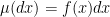Suppose we wish to obtain samples from some probability measure on . If has a sufficiently well-behaved density with respect to the Lebesgue measure, i.e., , then we can use the (overdamped) continuous-time Langevin dynamics, governed by the Ito stochastic differential equation (SDE)

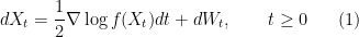
where the initial condition is generated according to some probability law , and is the standard -dimensional Brownian motion. Let denote the probability law of . Then, under appropriate regularity conditions on , one can establish the following:

• is the unique invariant distribution of (1), i.e., if , then for all .
• converges to in a suitable sense as — in fact, it is often possible to show that there exists a constant that depends only on , such that one has the exponential convergence to equilibrium

  

  for some distance between probability measures on .

In this sense, the Langevin process (1) gives only approximate samples from . I would like to discuss an alternative approach that uses diffusion processes to obtain exact samples in finite time. This approach is based on ideas that appeared in two papers from the 1930s by Erwin Schrödinger in the context of physics, and is now referred to as the Schrödinger bridge problem.

We will now assume that the target probability measure has a density with respect to the canonical Gaussian measure on , i.e.,

We will also assume that is everywhere strictly positive. Our goal is to construct an Ito process governed by the SDE

starting at , such that:

• has probability law ;
• , the probability law of the process , is optimal in the sense that, among all the diffusion processes with values in starting at the origin at and having the marginal distribution at , it remains “as close as possible” to the standard Brownian motion in the sense to be made precise below.

Note that the drift in (2) is time-dependent. This problem has been studied from many angles, and the optimal drift has an explicit form. My goal here is to give what is, to the best of my knowledge, a somewhat new and rather transparent derivation of the solution to the Schrödinger bridge problem. The main idea is based on a rather neat trick that I picked up from a paper by Hiroshi Ezawa, John Klauder, and Larry Shepp (although it was already present in some form in an earlier short paper by Václav Beneš and Shepp). The presentation will be rather informal, but every step can be made rigorous.

1. The Schrödinger bridge problem

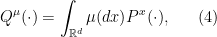
The basic problem can be stated as follows. Let denote the space of continuous functions (paths) from into , and let denote the canonical coordinate process on : For any , . Let denote the Wiener measure on , under which is the standard -dimensional Brownian motion on . Given any probability measure on , we will denote by the marginal probability law of the value of the path at time . With this, we consider the set

where denotes the Dirac probability measure on centered at the origin. Our goal is to find

where denotes the relative entropy between two probability measures on . We will need to do two things: (a) show that exists and is unique, and (b) show that it is the probability law of a diffusion process governed by an Ito SDE of the form (2).

To take care of (a), all we need is the chain rule for the relative entropy. Fix an arbitrary ; without loss of generality, we can assume that is absolutely continuous with respect to the Wiener measure , i.e., . The chain rule then gives

where (respectively, ) denotes the conditional probability law of given under (respectively, ). The conditional probability measure is well-known, and gives the probability law of the Brownian bridge process, i.e., the standard Brownian motion pinned to the point at . Now, since , we have , whereas for the Wiener measure . Thus, we have the following for the right-hand side of (3):

where equality holds if and only if almost everywhere. This immediately implies two things:

• ;
• the above infimum is attained by the probability measure

  

  i.e., by the -mixture of the Brownian bridge processes .

From (4), it is easy to obtain an explicit expression for the Radon–Nikodym derivative : Let be an arbitrary bounded measurable real-valued function on . Then, using the fact that , (4), and the law of iterated expectation, we can write

where the first equation is due to the fact that , in the second equation we have used the fact that the conditional laws and coincide, and in the last equation denotes the standard Brownian motion process with process law . That is, the Radon–Nikodym derivative of with respect to , as a function of the path , depends only on the terminal point and takes the form

where, as we recall, denotes the density of the target measure with respect to the standard Gaussian measure on . Thus, the optimal measure is simply the law of the standard -dimensional Brownian motion on , “conditioned” to have law at .

2. The gradient ansatz and the Girsanov transformation

In principle, (5) already tells us that we can obtain samples from by “reweighting” the Brownian paths using the weight factor that depends only on . What we are after, however, is something different: Instead of reweighting, we would like to construct a “transport” map such that , i.e., the optimal measure is the pushforward of the Wiener measure by :

for any bounded measurable . Moreover, we want this to be such that the “transported” process is an Ito diffusion process. In order to construct such a map, we will use a fundamental result in stochastic calculus, the Girsanov theorem, which gives the necessary and sufficient condition for a probability measure on to be absolutely continuous with respect to the Wiener measure .

In order to make use of it, we will first make the gradient ansatz, i.e., we will assume that the diffusion process we seek is governed by an Ito SDE of the form

where denotes the gradient with respect to the space variable. Then we will show that we can choose a suitable function which is twice continuously differentiable in and once continuously differentiable in , such that the probablity law of the resulting process will be given by . To motivate the introduction of the gradient ansatz, it is useful to compare the SDE (6) with the Langevin SDE (1) — the latter has a time-invariant drift given by the gradient of the log-density of with respect to the Lebesgue measure, while in the former we are using a time-varying drift since our goal is to obtain a sample from at time , and intuition suggests that a nonstationary process is needed to make this work.

At any rate, denoting by the probability law of the process (6), we can use the Girsanov theorem to write down the Radon–Nikodym derivative of with respect to :

Comparing (7) with (5), the path forward is now clear: We need to show that can be chosen in such a way that the right-hand side of (7) is equal to . This is where the Ezawa–Klauder–Shepp trick comes in. The key idea is to eliminate the Ito integral in (7) and then to reduce the problem to solving a suitable partial differential equation (PDE).

Let us define the process by . Ito’s lemma then gives

where is the Laplacian. Integrating and rearranging, we obtain

Substituting this into (7) and using the definition of gives

If we are to have any hope of reducing the right-hand side to an expression that depends only on , we need to ensure that the integral over is identically zero.

3. The PDE connection

One way of guaranteeing this is to assume that solves the PDE

for all , subject to the terminal condition for some strictly positive function to be chosen later. Assuming that such a exists, we will then have

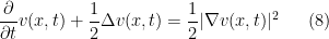
which means that should be chosen in such a way that for all . Now, the PDE (8) is nonlinear in due to the presence of the squared norm of the gradient of on the right-hand side. However, it is known from the theory of PDEs that we can convert it into a linear PDE that can be solved explicitly; this is accomplished by making the logarithmic (or Cole–Hopf) transformation . It is then a straightforward if tedious exercise in multivariate calculus to show that the function solves a much nicer linear PDE

on subject to the terminal condition . The solution of (10) is given by the Feynman–Kac formula, one of the remarkable connections between the theory of (parabolic) PDEs and diffusion processes: For any and ,

The proof of (11) is a simple application of Ito’s lemma: for any ,

Taking the conditional expectation given and using the fact that solves (10), we obtain (11).

Going back to (8), we can now write

and, in particular, . Substituting all of this into (9) gives

which means that we should evidently choose so that . Moreover, using the known Gaussian form of the transition probability densities of the Brownian motion, we can give the drift in (6) explicitly as

where is distributed according to the canonical Gaussian measure . This is known as the Föllmer drift (see this paper by Ronen Eldan and James Lee for more information and for further references).

4. The optimal control formulation

Those of you who are familiar with the theory of controlled diffusion processes should recognize the PDE (8) as the Hamilton–Jacobi–Bellman equation for the value function of a certain finite-horizon optimal stochastic control problem. While I do not want to get too much into details, I will sketch the basic idea. The first step is to use the identity

where the minimum is achieved uniquely by , to rewrite (8) in the equivalent form

for with . The stochastic control connection is as follows: We seek an adapted control process to minimize the expected cost

where denotes expectation with respect to the controlled diffusion process

Here, the integral is the control cost, while is the terminal cost at . It can then be shown using the so-called verification theorem in the theory of controlled diffusions that the solution of the PDE (12) gives the value function (or the optimal cost-to-go function)

so that, in particular, . Here, the idea is that we add the drift to the standard Brownian motion to steer the process towards the target distribution at , while keeping the total “control effort” small. Of course, from the preceding derivations we know that , and that the optimal control is of the state feedback form, given explicitly by the Föllmer drift. Moreover, one can show using the Girsanov theorem that every can be realized as a controlled process of the form (14) for some admissible drift , so that has law and

This implies, in turn, that the Föllmer drift that gives the optimal measure is the most efficient control, in the sense that the sum of the expected control cost and the expected terminal cost is identically zero, and therefore none of the control effort is wasted along the way. Of course, one could have started with this optimal control formulation (as I do in this paper with Belinda Tzen), but I feel that the above derivation is more “elementary” in the sense that it does not rely on any specialized knowledge beyond basic stochastic calculus.

Machine learning is about enabling computers to improve their performance on a given task as they get more data. Can we express this intuition quantitatively using information-theoretic techniques? In this post, I will discuss a classic paper by David Haussler, Michael Kearns, and Robert Schapire that (to the best of my knowledge) took the first step in this direction. In this post, I will describe some of their results, recast in a more explicitly information-theoretic way.

We will stick to the setting of binary classification: we have a feature space (which is completely arbitrary) and a binary label space . Let be a class of functions , which we will call the hypothesis space. These functions are our models for the relationship between features and labels, which we wish to learn from data. In order to focus on the essential aspects of the problem, we will adopt the Bayesian approach and assume that the “true” model is a random element of with a given distribution . We assume that the learning agent knows , so we can think of this distribution as the learner’s prior. Training data consist of input-output pairs , where . Here, each is an arbitrary point of , and for now we will treat as an individual sequence. The labels , though, are random and given by , where is the model drawn by Nature from .

The learning agent receives the training data sequentially: at each time , it has access to . Let us denote the pair by . The learning task is: given the next input , predict the value . A learning algorithm is a sequence of possibly randomized mappings : at each time , the learning agent uses all available training data to generate a prediction for the label of . After generating the prediction, the learning agent observes the true . We are interested in the probability that makes an error at time :

We will refer to the function as the learning curve of [note that it depends on the sequence of inputs supplied to the learning agent during learning].

How can we measure the learner’s progress? Let’s write out the causal ordering of all the random variables generated in the process of learning:

Here, has distribution , are determined by the learning algorithm , and are determined by and . Let us denote the joint distribution of all of these variables by . When the learning agent observes at time , we can quantify its information gain relative to time by

It’s not hard to see that is nonnegative because (information at time ) includes . The expected information gain is given by

the conditional mutual information between and given . For our purposes, it will be convenient to express the information gain in terms of a certain quantity called the volume ratio, which quantifies the rate at which the learning agent can zero in on the true model as more observations keep arriving.

To that end, let us first observe that, at time , the agent can localize the unknown model to the set

This set is known in learning theory as the version space at time . It is easy to see that the version spaces are nested: . Clearly, for all , and for any

This implies, in particular, that

and therefore that

where . Since , we expect that each training sample shrinks the version space, and that the learning curve of any good learning algorithm should be controlled by the rate at which decreases. For future convenience, let us define the volume ratio at time :

Note, by the way, that since , we have

Consequently,

We are going to use binary algorithms, so the units of all information quantities are bits.

Now let’s get down to business. Following Haussler et al., we will consider the following two learning algorithms:

1. The Bayes algorithm : at time , it partitions the version space into two disjoint subsets

   

   and then predicts

   

   The Bayes algorithm is optimal in the sense that it minimizes the probability of incorrectly predicting given all available information. However, it is an improper learning algorithm in the sense that the function will not, in general, be an element of .

2. The Gibbs algorithm : at time , it draws a random and predicts

   

   The Gibbs algorithm is suboptimal, but, unlike the Bayes algorithm, the function does belong to by construction.

Now let’s analyze their learning curves:

1. The Bayes algorithm will make a mistake whenever , i.e., whenever . Indeed, using the fact that, by definition of the version space,

   

   we have

   

   Thus, if , then , and so . On the other hand, if , the Bayes algorithm will be correct: . Finally, if , then the Bayes algorithm will make a mistake with probability . Therefore,

   

   where we have defined the function

   

2. The Gibbs algorithm will make a mistake whenever is not in the version space . Since is drawn from the posterior distribution of given , we have

   

Before stating and proving the main result, we need to collect some preliminary facts. First of all, the volume ratio is always bounded between and . Moreover, we have the following useful formula: for any function ,

(the proof is by conditioning on and using the law of iterated expectation).

Theorem 1 We have the following bounds for the Bayes and the Gibbs algorithms:

and

where is the inverse of the binary entropy function .

Remark 1 Equation (2) shows that the error probability of the Bayes algorithm at time can be bounded below by a function of the expected information gain at time . It also shows that the error probability of the Gibbs algorithm is at least as large as that of the Bayes algorithm. On the other hand, Equation (3) gives an upper bound on the error performance of the Bayes algorithm in terms of the expected information gain, and it also shows that the error of the Gibbs algorithm is at most twice as large as that of the Bayes algorithm.

Proof: We start by obtaining the following alternative expressions for the error probabilities of the two algorithms, as well as for the expected information gain:

Using (1) with , we have

This shows, in particular, that the average information gain due to receiving another training sample is no more than one bit.

With , we have

where we have used the fact that, for any ,

Another way to arrive at this expression is by using the following fact: Suppose we have a biased coin with probability of heads equal to . The best prediction of the outcome of a single toss of that coin, with respect to the Hamming loss , is to predict heads if and tails otherwise. The expected loss in that case is equal to . The problem of predicting given and is equivalent to the above guessing problem with .

Finally, with , we have

Again, if we consider the problem of guessing the outcome of tossing a coin, we can think of the following suboptimal scheme: guess with probability and with probability (i.e., just mentally simulate the coin toss). The probability of error is exactly , which is also twice the variance of a random variable. Reasoning conditionally on , we see that the Gibbs algorithm is exactly this scheme with .

We will also use the following chain of easy-to-prove inequalities: for any ,

We start by proving the lower bound, Equation (2). First, note that, for any ,

Moreover, the function is convex. Therefore,

The upper bound, Equation (3), follows by taking in (4) and then taking expectations.

Now let’s see what happens when we have to do this over and over again: at each time , the learning agent gives a prediction , observes , updates , etc. What can we say about the expected fraction of mistakes? Given a learning algorithm , the quantity of interest is

for each . In order to get a handle on this quantity, we will need some Vapnik-Chervonenkis combinatorics. Given the sequence of input instances, let denote the set of all distinct elements of the tuple . Say that two hypotheses are equivalent if for all . This defines an equivalence relation on , so we can split it into equivalence classes . Here, the number of equivalence classes depends on and on . How many such classes can we have? Let us order the elements of arbitrarily, say by , where . Each can be associated with a binary string . Then and are in the same equivalence class if and only if they give rise to the same binary strings:

Consequently,

For any subset , let us define in the obvious way: if , then we let . Let be the largest integer , such that

for all with . A deep result, commonly known as the Sauer-Shelah lemma (see here for some fascinating history), then says that

Now we are ready to state and prove the following:

Theorem 2

Proof: We have

From the definition of the version spaces, it is immediate that is the equivalence class containing the “true” model . In other words, there exists some random , such that . Consequently, we can write

We can recognize the quantity in the last line as the Shannon entropy of the index : that is,

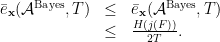
Now, since takes values in , we can invoke the Sauer-Shelah estimate (5) to get

The claimed bound (6) follows.

If is a Vapnik-Chervonenkis class with VC dimension , then we immediately obtain:

Corollary 3

Models of complex systems built from simple, locally interacting components arise in many fields, including statistical physics, biology, artificial intelligence, communication networks, etc. The quest to understand and to quantify the fundamental limits on the ability of such systems to store and process information has led to a variety of interesting and insightful results that draw upon probability, combinatorics, information theory, discrete and continuous dynamical systems, etc. In this post, I would like to focus on a model of distributed storage that was analyzed in 1975 by Donald Dawson in a very nice paper, which deserves to be more widely known.

The system Dawson analyzed is an instance of a Probabilistic Cellular Automaton (PCA), i.e., a system consisting of a discrete collection of nodes, each of which has a discrete state. The configuration of the automaton at each time is specified by listing the state of each node. The state of each node at time is determined stochastically by its own state, as well as by the states of its neighbors, at time , independently of everything else. One of the key questions in the theory of PCAs is whether a given automaton is ergodic, i.e., if its configuration eventually “forgets” the initial condition. Thus, Dawson’s result is a sufficient condition for ergodicity of a PCA.

Now let’s move on to precise definitions. Consider an undirected graph . The neighborhood of a vertex , denoted by , is the set of all vertices that are connected to by an edge. We will also denote the set consisting of and all of its neighbors by . Let us fix a finite alphabet ; for each vertex , let denote a copy of . A configuration is an assignment of a symbol to each vertex . Thus, is the space of all configurations. We will denote a generic configuration by ; for any set , we will denote by the natural projection of onto : .

Now let’s consider the following model of a distributed one-bit memory cell. Let be a random variable, which is the bit we wish to store. We also pick two probability measures and on . Given , we draw the initial configuration at random according to . We allow arbitrary correlations between the different ‘s, so our storage is distributed in this sense. Now let’s suppose that the state of each vertex evolves stochastically in discrete time according to a local Markov model: for each , we have a channel (random transformation) with input alphabet and output alphabet . Then the configuration at time evolves according to the law

with the initial conditions , , and , . Thus, we end up with a Markov chain

where at each time the evolution from to is also Markov “in space:” the state of vertex at time is determined only by the states of the neighbors of at time , i.e., for each and , we have a Markov chain

Now the question is: does the configuration at an arbitrary time retain any information about ? One way to answer this is to pick an arbitrary finite set and to examine the evolution of the mutual information , where

If we can show that there exists some such that for all and at least one nonempty , then our memory cell is capable of storing one bit. If, on the other hand, as for every finite , then eventually the memory cell will forget .

1. Dawson’s impossibility result

Roughly speaking, Dawson proved the following: if the local channels are sufficiently noisy and if the graph is sufficiently sparse, then the mutual information will decay to zero exponentially fast. In order to state his result precisely, we need some preliminary definitions. First of all, in order to quantify the noisiness of each channel , Dawson introduces the following quantity, which he calls the transmission coefficient of :

where the supremum is over all Markov chains , where , the channel from to is arbitrary, and the channel from to is given by . Moreover, let . Clearly, for every , by the data processing inequality. Consequently, .

Remark 1 Dawson’s definition of the transmission coefficient is reminiscent of the best constant in the data processing inequality of Erkip and Cover (corrected by Anantharam et al.): to define that constant in our setting, one would fix a distribution and let

where the supremum is over all Markov chains satisfying the constraints and . The difference is that in (2) we constrain the marginal distribution of and the stochastic kernel , whereas in (3) we constrain the marginal of and the kernel . As shown by Anantharam et al.,

where the supremum is over all marginal distributions of distinct from , and denotes the marginal distribution of when . Both and measure the “noisiness” of , but in different ways. In particular, the motivation behind Dawson’s definition is as follows: At any time , the state of a given node at time depends only on and not on anything else. Thus, if boundary condition, i.e., the configuration of all the nodes except for and its neighbors, is “frozen” at some value , then the amount of information about that node will receive at time will be controlled by the quantity

which, by definition, is no more than . We will elaborate on this point later on.

Also, Dawson assumes that has bounded degree, i.e.,

Now we are in a position to state the following:

Theorem 1 (Dawson) For any finite set ,

Thus, if , then as , and the convergence is exponentially fast.

2. The proof

The proof of Theorem 1 consists of several steps. The first step gives an upper bound on the information value of the state at a given node if we already observed the states of some other nodes. This bound is stated in Lemmas 2 and 3 below.

Lemma 2 Fix two arbitrary, possibly empty finite sets . Then, for any ,

Proof: We begin by noting that, since ,

is a Markov chain. Now, for any fixed choices of the configurations and , consider two probability distributions and of :

From (6), if we consider a channel from to with transition probabilities given by , and then let be the output of with input , then

and is a Markov chain satisfying the conditions in the definition (2) of the transmission coefficient . Therefore,

Taking the expectation with respect to and , we obtain (5).

Lemma 3 For any finite set , any , and an arbitrary (possibly empty) finite set ,

Proof: Using the chain rule for mutual information and Lemma 2,

Now let’s examine the mutual information . Let us use the chain rule to write the conditional mutual information in two ways:

Therefore, we can write

Substituting this into our bound on , we obtain the statement of the lemma.

The main message of Lemma 3 can be stated more succinctly if we introduce shorthand notation

\and

for all finite, possibly empty sets and for all , where we also let

for all finite sets . A nice way to think about the above definitions is in terms of prediction and correction steps in Bayesian filtering: Eq. (7) corresponds to prediction since it quantifies the amount of information about that the nodes in will contain at time given what we know about the state of the nodes in some other set at time , while Eq. (8) quantifies the impact of knowing the state of the nodes in at time , and so represents correction. Moreover, we can write the bound of Lemma 3 as

for any , any , and any .

The second step of the proof is to show that the exponential decay of information, according to Eq. (4), is a consequence of (9). To that end, Dawson employs a clever inductive argument. Let denote the collection of all finite subsets of , and for any define a set function by

The quantity defined in Eq. (8) can be computed in terms of : indeed, by the chain rule we have

In addition, if we know , we can also compute :

Moreover, using our knowledge of and the fact that for all , we can do the following: Let us fix an arbitrary node . Then, from (9), we derive

Fixing another node , we have

where the first step uses (9); the second uses our bound on ; in the third, we add and subtract ; and the last step uses the chain rule. Continuing inductively, we see that, for any ,

In particular, using the formula with , we obtain

The final step is to complete the proof using the fact that . Since is binary, . Therefore,

This can be interpreted as follows: if we define the specific information at time by

then . Now, we write

where the first step follows from (10); the second uses (11); the third step is by (over)counting; the fourth step uses the fact that for every ; and the remaining steps are simple combinatorics. What we have shown is that the specific information at can be bounded as . Thus, if , then in one step the specific information will strictly decrease. Iterating, we get the bound

If , then as . This completes the proof of Theorem 1.

1. The 2014 IEEE North American Summer School on Information Theory will take place June 18-21, 2014 at the Fields Institute in Toronto, Canada.

2. For those of you who use Matlab or Octave, there is a new Information Theoretical Estimators (ITE) toolbox, an open-source toolbox “capable of estimating many different variants of entropy, mutual information, divergence, association measures, cross quantities, and kernels on distributions.” Some more details are available in the guest post by the toolbox’s creator, Zoltán Zsabó, at the Princeton Information Theory b-log.

Just a quick note for my reference, but it may be of interest to others.

Let denote the size of the largest code over a -ary alphabet that has blocklength and minimum distance . The well-known Gilbert-Varshamov bound says that

where

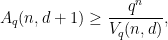
is the volume of a Hamming ball of radius in . The usual way of arriving at the GV bound is through a greedy construction: pick an arbitrary codeword , then keep adding codewords that are at Hamming distance of at least from all codewords that have already been picked. When this procedure terminates, the complement of the union of the Hamming balls of radius around each of the codewords should be empty — otherwise, you will have at least one more codeword at distance of at least from the ones already picked, and this would mean that the procedure could not have terminated.

As it turns out, there is another way of deriving the GV bound using graph theory that I have learned from a nice paper by Van Vu and Lei Wu. They use this graph-theoretic interpretation to arrive at an asymptotic improvement of the GV bound. Their result, which I will not go into here, extends an earlier result by Tao Jiang and Alex Vardy for binary codes. As far as I can tell, the graph-theoretic ideas go back to the Jiang-Vardy paper as well.

In order to proceed, we need some definitions and a lemma. Let be an undirected graph. A set of vertices is called independent if no two vertices in are connected by an edge. The independence number of , denoted by , is the cardinality of the largest independent set. The following lemma is folklore in graph theory:

Lemma 1 Suppose that is -regular, i.e., every vertex has exactly neighbors. Then

Proof: Let be a maximal independent set. Any vertex is connected by an edge to at least one , because otherwise would have to be included in , which would contradict maximality. Therefore, there are at least edges with one vertex in and another vertex in . On the other hand, because is -regular, there can be at most such edges. This means that

Rearranging, we get (1).

Now let us construct the following graph (what Jiang and Vardy call the Gilbert graph): associate a vertex to each word in , and connect two vertices by an edge if and only if the Hamming distance between the corresponding words is at most . This graph has vertices, and each vertex has degree . Moreover, there is a one-to-one correspondence between independent sets of vertices and -ary codes of length and minimum distance at least , and the independence number of the Gilbert graph is equal to . The bound (1) is then precisely the GV bound.

Briefly, the Vu-Wu improvement of the GV bound exploits the deep fact that, when the neighborhood of any vertex in a -regular graph is very sparse (in the sense that it has a lot fewer than edges), the lower bound (1) can be significantly tightened. Apparently, actually counting the number of edges in such a neighborhood of any vertex of the Gilbert graph (by regularity, we may as well look at the neighborhood of the all-zero word) is rather complicated; Vu and Wu instead look at a suitable asymptotic regime when is large and for some and replace exact combinatorial bounds by entropy bounds.

… circa 1935. Here is a quote from Single-Story America (translated as Little Golden America), an American travelogue by Ilya Ilf and Yevgeny Petrov:

There is a whole book of readymade telegrams, long and convincing, lavishly composed telegrams for all occasions. Sending such a telegram costs only twenty-five cents. You see, what gets transmitted over the telegraph is not the text of the telegram, but simply the number under which it is listed in the book, and the signature of the sender. This is quite a funny thing, reminiscent of Drugstore Breakfast #2. Everything is served up in a ready form, and the customer is totally freed from the unpleasant necessity to think, and to spend money on top of it.

Typical set encoding, anyone?

Of the five plenary talks at this year’s ISIT, two were about concentration of measure: Katalin Marton’s Shannon lecture on “Distance-divergence inequalities” and Gabor Lugosi’s talk on “Concentration inequalities and the entropy method” the next morning. Since the topic of measure concentration is dear to my heart, I thought I would write down a few unifying themes.

When we speak of concentration of measure, we mean the following. Let be a random variable taking values in some metric space . Then we say that (or, more correctly, the distribution of ) has the concentration property if, for any set such that , we have

Here, is the distance from the point to the set :

Another way to express (1) is as follows: for any set and any , define the -blowup of by

Then has the concentration property if

In other words, has the concentration property if any set containing with not too small a probability can be “blown up” to contain with near-certainty.

Here are two classic examples of concentration:

1. Gaussian distribution in Euclidean space. Let and take — the usual Euclidean distance. Let be a standard -dimensional Gaussian random variable, i.e., , where is the identity matrix. Then for any we have

   

2. Uniform distribution in Hamming space. Let be the Hamming cube equipped with the normalized Hamming distance

   

   that counts the fraction of bits in which and disagree. Let have the uniform distribution on , i.e., for all . Then

   

These two examples suggest that we should aim for “hard” statements in the form of sharp bounds on the concentration function

as opposed to merely “soft” statements of the form as . The $64,000 question is: how do we get such bounds?

There are two ways to accomplish this goal, and the main idea underlying these two ways is to replace sets with some other objects that are hopefully easier to handle. The first way is to replace sets by probability measures, the second is to replace them by functions. Here is what I mean:

Fix a set with . Let denote the distribution of , and let denote the conditional distribution of given . That is, for any (measurable) set we have

I am using the subscript notation instead of the more usual to indicate the fact that is a probability measure in its own right. In this way, we can associate to each non-null set a probability measure . Now, here is a very simple observation that turns out to be very consequential:

This is very easy to prove: for any set we have

so is absolutely continuous with respect to with the Radon-Nikodym derivative . Therefore, by definition of the divergence,

So if we are interested in bounding the probabilities of various sets , we may hope to get some mileage out of the relationship (2).

On the other hand, we may also associate to a set with the function

This function is Lipschitz: for any ,

where the last step is by the triangle inequality. Interchanging the roles of and , we get the Lipschitz property. Moreover, let us consider the random variable , where is our original -valued random variable. Then we immediately notice two things:

1. For any , .
2. If , then is a median of , in the sense that

   

   (the second inequality is obviously true since is nonnegative with probability ).

These two observations suggest that we may obtain concentration bounds by bounding the probability that a given Lipschitz function of deviates from its median by more than . In fact, it is easy to derive an alternative expression for the concentration function :

where denotes any median of . We already showed, by passing from to , that is bounded from above by the quantity on the right-hand side of (3):

To prove the reverse inequality, fix any -Lipschitz function and consider the set , where is any median of . Then, by definition,

Moreover, if we consider the -blowup

then for any and any we must have

where the last step is by the Lipschitz property of . Consequently, by definition of the concentration function,

By passing to the functional viewpoint, we obtain another equivalent characterization of the concentration property: a random variable taking values in a metric space has the concentration property if real-valued Lipschitz functions are “nearly constant.”

Let’s look at the first, probabilistic viewpoint, which was born out of a 1996 breakthrough paper by Marton. Given a metric space , let us define the Wasserstein distance (or transportation distance) between any two probability measures and on it:

where the infimum is over all jointly distributed random variables , such that and . Now consider a random variable , for which we wish to establish concentration. What Marton showed is the following: Suppose the distribution of satisfies the transportation inequality

for some constant . Then has the concentration property, and moreover

Marton’s proof is breathtakingly beautiful. Consider any two sets with . Recalling our notation for conditional distributions, we can write

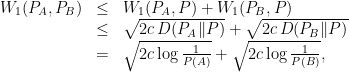
where in the first step we have used the triangle inequality, in the second we have used the fact that satisfies the transportation inequality (4), and in the last step we have used the formula (2). Now suppose that and let for some , where denotes set-theoretic complement. Then we can show that . On the other hand,

Combining these facts gives us the bound

that holds for all . If , then we get

so we indeed have concentration and a sharp bound on , at least for large enough values of . The main message here is that, in order to study concentration, it suffices to work on the level of probability measures and to focus one’s effort on showing that the distribution of satisfies a suitable transportation inequality. Since Marton’s original work, there have been many refinements and extensions, which I will not go into here. One such result, due to Sergey Bobkov and Friedrich Götze, says that satisfying a transportation inequality (4) is equivalent to the Gaussian concentration property

Now let’s look at the complementary functional viewpoint. Recall that we seek tight upper bounds on deviation probabilities of the form

It is easier to work with means instead of medians, and indeed it can be shown that concentration around the mean is equivalent to concentration around any median. So let’s focus on the mean. Let , as before, be a random variable over some metric space , and consider a Lipschitz function such that . We can apply the well-known Chernoff trick: for any we have

Now the whole affair hinges on the availability of tight upper bounds on the logarithmic moment-generating function . The entropy method, which was the subject of Gabor Lugosi’s plenary, is the name for a set of techniques for bounding by means of various inequalities involving the relative entropy between various tilted distributions derived from and itself. The entropy method has roots in the work of Michel Ledoux, who in turn distilled it from some very deep results of Michel Talagrand.

The simplest version of the entropy method goes something like this. Let us define, for any , the tilted distribution via

(assuming, of course, that exists and is finite). Then we have

Integrating and using the fact that , we get

Now suppose that we can bound for some . Then from (5) we have

which in turn gives the Gaussian tail bound

This is the so-called Herbst argument. Of course, I have glossed over the most nontrivial part — namely, showing that we can bound the relative entropy by a quadratic function of . Gabor’s talk contained numerous examples of how one could get such bounds in the special case when is an -tuple of independent random variables taking values in some base space , , and the function is not “too sensitive” to local modifications of its arguments. This takes us back to probability on metric spaces.

Here is one classic example. Suppose that our function has the bounded difference property, i.e., there exist some constants , such that changing the th argument of while keeping others constant will change the value of by at most :

We can express this more succinctly as a Lipschitz property of if we define the weighted Hamming metric

(we can assume without loss of generality that all the ‘s are strictly positive, because we can simply ignore those coordinates of that do not affect the value of ). Then the bounded difference property is equivalent to saying that is -Lipschitz with respect to this weighted Hamming metric. Moreover, it is possible to show that any product probability measure on the product space satisfies the transportation inequality

where the Wasserstein distance is computed with respect to the weighted Hamming metric (6), and . By the Bobkov–Götze result quoted above, this is equivalent to the concentration bound

This is the well-known McDiarmid’s inequality, which was originally derived using martingale techniques, but here we have arrived at it through a completely different route that took us back to where we started: concentration of Lipschitz functions around their means and/or medians, which (as we saw) is the same thing as the original, “stochastic-geometric” view of the concentration of measure phenomenon.

Endorse the petition to honor Claude Elwood Shannon with a United States Postal Service stamp on the 100th anniversary of his birth.